| Issue |
A&A
Volume 519, September 2010
|
|
|---|---|---|
| Article Number | A39 | |
| Number of page(s) | 24 | |
| Section | Interstellar and circumstellar matter | |
| DOI | https://doi.org/10.1051/0004-6361/200913906 | |
| Published online | 09 September 2010 | |
Online Material
Appendix A: Emission by an electric dipole in an infinite medium
We first study the electric field![\begin{figure}
\par\includegraphics[width=12cm,clip]{13906fgA1}
\end{figure}](/articles/aa/olm/2010/11/aa13906-09/img125.png)
|
Figure A.1:
Coordinate system and angles used to calculate the decomposition of the electric field |
| Open with DEXTER | |
Table A.1: Definition of axis, angles, and other notations.
The refractive index
![]() is complex if the medium j is absorbing. In the case of considering a non-absorbing medium j, the imaginary part of the index,
is complex if the medium j is absorbing. In the case of considering a non-absorbing medium j, the imaginary part of the index,
![]() ,
is zero. The refractive index
,
is zero. The refractive index
![]() is given by the relation A.1, and the wave vector
is given by the relation A.1, and the wave vector
![]() (in the direction of the observator) is linked to the complex refractive index by Eq. (A.2):
(in the direction of the observator) is linked to the complex refractive index by Eq. (A.2):
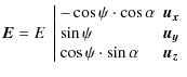
A.1 Polarization of the electric field
The electric field ![]() is perpendicular to the direction of observation
is perpendicular to the direction of observation ![]() and can be decomposed into two orthogonal components, i.e., two
polarizations: the s-polarized one is perpendicular to the observation
plane and the (p)-polarized one is in this plane:
and can be decomposed into two orthogonal components, i.e., two
polarizations: the s-polarized one is perpendicular to the observation
plane and the (p)-polarized one is in this plane:
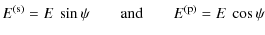
![$\displaystyle \vec{E} = E\ \left[\frac{1}{\sin \beta}\ \vec{u_{p}} - \frac{\cos \beta}{\sin \beta}\ \vec{u_{k}}\right]$](/articles/aa/olm/2010/11/aa13906-09/img148.png)
With Eqs. (A.7) and (A.8), we find
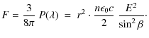
A.2 Radiant intensity in an infinite medium
The next equations show how to obtain the intensity from the electric field amplitude. We can linked the electric field to the irradiance that is the incident power of electromagnetic radiation at a surface, per unit area.
where
Radiant intensity (incident power per unit solid angle) I and irradiance created by the electric dipole ![]() are normalized as
are normalized as
where r is the radius of the sphere where the irradiance is calculated, and
| = | |||
| = | 
|
(A.12) |
| |
and |
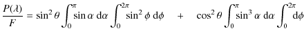
The normalization Eq. (A.11) let us obtain factor F:

|
|||

|
|||
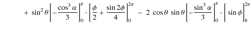
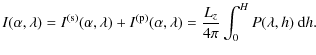
![$\displaystyle \frac{P(\lambda)}{F} = \sin^{2}\theta \bigg[-\cos \alpha \bigg]_{...](/articles/aa/olm/2010/11/aa13906-09/img173.png)
|
|||
|
|||
|
The radiant intensity emitted by one electric dipole
| |
(A.13) |
Consider now a luminescent layer of thickness H, and thus an ensemble of incoherently radiating electric dipoles having equal dipole moment
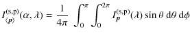
|
|||
The dipoles are located in the layer of thickness H; the total intensity emitted from this luminescent layer is thus obtained by integrating the product of
|
|||
|
|||
|
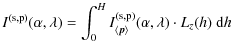
Let us consider now an absorbing medium with an index
- on the wave amplitude E:
E' = 
E' = 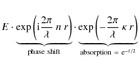
- on the wave intensity I:
I' 

I' = 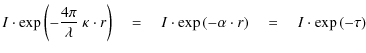
Appendix B: Effects of the interfaces of the film
In this appendix, we introduce the effects of the interfaces of the film and calculate the emission amplitude in a medium 1 by summing all the transmitted components (of each polarization), taking the phase shift and absorption due to propagation in each medium into account. As a result, the radiation pattern are obtained: it is the angular distribution of the light emitted by the film into the half-space 1.
Until now, we have considered an infinite medium. We now
consider three different homogenous media (medium 0 is a film between
semi-infinite media 1 and 2) and their interfaces. The
emitting dipole ![]() is now located in the film 0. Our aim is to determine the radiation transmitted in medium 1 under the angle of observation
is now located in the film 0. Our aim is to determine the radiation transmitted in medium 1 under the angle of observation ![]() .
.
We separate the light transmitted in medium 1 into two beams: the
direct beam D is the one emitted directly in the direction of
medium 1 (with an emission angle
![]() given by the angle of observation
given by the angle of observation
![]() and the Snell-Descartes relation of refraction). The reflected beam R
is the beam that is first directed toward medium 2 and reflected off
the interface 0/2 before being transmitted in medium 1. Each of these
beams is reflected multiple times between each interface of the
film 0. In this paragraph, we see that interference effects appear
because of these multiple reflections and also because of the sum of
the two different beams, D and R. This latter case of interference is known as the wide-angle effect.
and the Snell-Descartes relation of refraction). The reflected beam R
is the beam that is first directed toward medium 2 and reflected off
the interface 0/2 before being transmitted in medium 1. Each of these
beams is reflected multiple times between each interface of the
film 0. In this paragraph, we see that interference effects appear
because of these multiple reflections and also because of the sum of
the two different beams, D and R. This latter case of interference is known as the wide-angle effect.
![\begin{figure}
\par\includegraphics[width=12cm,clip]{13906fgB1}
\end{figure}](/articles/aa/olm/2010/11/aa13906-09/img196.png)
|
Figure B.1:
Schematic diagram of the emission geometry for a dipole embedded in a
thin film (medium 0), at a distance h from the surface, for an emission
angle
|
| Open with DEXTER | |
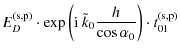
B.1 The direct beam D
We first consider the the direct beam D, with its multiple reflection back and forth in layer 0, transmitted in medium 1 as shown in Fig. B.2:

|
|
= | 
|
|
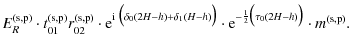
![$\displaystyle \times \left[1 + \left(r_{01}^{\rm (s,p)} \ r_{02}^{\rm (s,p)} \ ...
...n \alpha_{1} \big)}_{\rm external\ phase\ shift} \right) + (...)^2 + ...\right]$](/articles/aa/olm/2010/11/aa13906-09/img201.png)
|
|
|
= | (B.1) | |
![$\displaystyle \times \left[ 1 + \sum_{l=1}^\infty \left( r_{01}^{\rm (s,p)}\ r_...
...\tau_{0}(H) \big)\ \exp \big({\rm i}\ \delta_{1}(H) \big)\ \right)^{l} \right].$](/articles/aa/olm/2010/11/aa13906-09/img203.png)
|
The following notations are used to lighten expressions.
Remark: ![]() is defined with a factor
is defined with a factor
![]() to obtain a power attenuation of
to obtain a power attenuation of
![]() .
.
| absorption: | |||
| phase shift: | |||
|
|||
where
Hence, one derives
|
(B.2) | ||
|
![\begin{figure}
\par\includegraphics[width=12cm,clip]{13906fgB2}
\end{figure}](/articles/aa/olm/2010/11/aa13906-09/img217.png)
|
Figure B.2: Schematic diagram of the emission geometry for the direct beam D. |
| Open with DEXTER | |
B.2 The reflected beam R
![\begin{figure}
\par\includegraphics[width=12cm,clip]{13906fgB3}
\vspace*{7mm}
\end{figure}](/articles/aa/olm/2010/11/aa13906-09/img218.png)
|
Figure B.3: Schematic diagram of the emission geometry of the reflected beam R. |
| Open with DEXTER | |

|
|
= | 
|
|
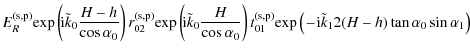
![$\displaystyle \times \left[1 + \left(r_{01}^{\rm (s,p)} \ r_{02}^{\rm (s,p)} \ ...
...{k}_{1} 2H \tan \alpha_{0} \sin \alpha_{1} \big) \right) + (...)^2 + ...\right]$](/articles/aa/olm/2010/11/aa13906-09/img222.png)
|
|||
| = | |||
| = | 
|
(B.3) |
B.3 Combination of the D and R beams
We calculated the expression of the electric field amplitude transmitted in medium 1 of the direct beam
![]() and of the reflected beam
and of the reflected beam
![]() ,
for each polarization, (s) and (p). These amplitudes are exprimed as a function of
,
for each polarization, (s) and (p). These amplitudes are exprimed as a function of
![]() and
and
![]() ,
which are the electric field amplitude emitted by an electric dipole in the direction
,
which are the electric field amplitude emitted by an electric dipole in the direction
![]() and
and
![]() ,
respectively:
,
respectively:

The Eqs. (A.9) and (A.10) give the influence of the angle
| (B.4) | |||
| (B.5) | |||
| (B.6) | |||
To combine the electric fields in medium 1 due to the direct and reflected beams
Let us consider the direction of the vectors

The reflection at the interface 0/2 of the reflected beam changes the sign of
- in the same direction for the s-polarization
- in opposite direction for the p-polarization.
| and: |
|
|
= | ||
![$\displaystyle \left. \pm_{(p)}^{\rm (s)} \ E_{R}^{\rm (s,p)} \cdot r_{02}^{\rm ...
...ta_{1}(H-h)\big)\big] \cdot \exp \big[- \frac{1}{2} \tau_{0}(2H-h)\big] \right]$](/articles/aa/olm/2010/11/aa13906-09/img254.png)
|
|||
| = | (B.7) |
where
B.3.1 s-polarized
| (B.8) | |||
B.3.2 p-polarized
| (B.9) |
B.4 Radiation pattern
The radiation pattern is the angular distribution of the light emitted by the source ![]() located in layer 0 into the half-space 1, expressed by
located in layer 0 into the half-space 1, expressed by
![]() the intensity (
the intensity (
![]() )
emitted in the direction given the angles
)
emitted in the direction given the angles
![]() into the half-space 1.
into the half-space 1.
| |
= | 
|
|
| = | (B.10) |
| |
= | ||
| = | (B.11) | ||
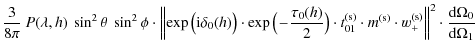
![$\displaystyle \times \left[\cos^{2} \theta\ \sin^{2} \alpha_{0}\ \left\Vert w_{...
...frac{1}{2} \sin{ 2 \theta} \cos \phi \sin{2 \alpha_{0}}\ w_{0}^{\rm (p)}\right]$](/articles/aa/olm/2010/11/aa13906-09/img274.png)
|
where:
B.4.1 Solid angle modification at the interface
The ratio
![]() represents the modification of solid angle when the medium changes,
represents the modification of solid angle when the medium changes,
![]() is the radiated power in medium i into the solid angle
is the radiated power in medium i into the solid angle
![]() .
When the wave goes through the interface i/j, the solid angle is modified and the power conservation is given by Eq. (B.12) (when the transmission coefficient is 1):
.
When the wave goes through the interface i/j, the solid angle is modified and the power conservation is given by Eq. (B.12) (when the transmission coefficient is 1):
This is the origin of the factor
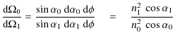
|
(B.12) |
using the derivative of the Snell-Descartes law.
B.4.2 Random orientation of the dipoles
To take a random orientation for the electric dipoles embedded in the film account, the intensity is averaged over ![]() and
and ![]() .
The geometry is thus no more dependent on the angle
.
The geometry is thus no more dependent on the angle ![]() ;
I1 is now only depending on the angle of observation
;
I1 is now only depending on the angle of observation ![]() .
.
![]() ,
which is the total power emitted in all directions of the space, at the wavelength
,
which is the total power emitted in all directions of the space, at the wavelength ![]() ,
by a single dipole
,
by a single dipole ![]() at the depth h, does not vary with the direction of the dipole.
at the depth h, does not vary with the direction of the dipole.
The intensity (
![]() )
emitted by a film layer of thickness dh, at the film depth h, is
)
emitted by a film layer of thickness dh, at the film depth h, is
|
|||

|
|||
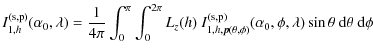
![$\displaystyle I_{1,h}^{\rm (s)}(\alpha_0, \lambda) = \frac{3}{32\pi^2}\ L_z(h)\...
...ht]_{0}^{\pi} \ \left[\frac{\phi}{2} - \frac{\sin (2\phi)}{4}\right]_{0}^{2\pi}$](/articles/aa/olm/2010/11/aa13906-09/img286.png)
|
|||
| (B.13) |
| |
= | 
|
|
![$\displaystyle \left. + \cos^{2} \alpha_{0}\ \Vert w_{+}^{\rm (p)} \Vert^{2}\!\!...
...\theta\ {\rm d}\theta \int_{0}^{2\pi}\!\!\!\!\! \cos \phi \ {\rm d}\phi \right]$](/articles/aa/olm/2010/11/aa13906-09/img290.png)
|
|||
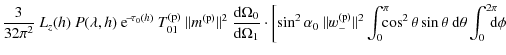
| = | ![$\displaystyle \frac{3}{32\pi^2}\ L_z(h)\ P(\lambda, h)\ {\rm e}^{\!-\! \tau_{0}...
...+ \cos^{2} \alpha_{0}\ \Vert w_{+}^{\rm (p)} \Vert^{2}\ \frac{4}{3}\ \pi\right]$](/articles/aa/olm/2010/11/aa13906-09/img291.png)
|
||
| = | (B.14) |
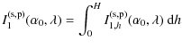
Finally, the specific radiant intensity in medium 1 and created by electric dipoles of random orientation at the film depth h is
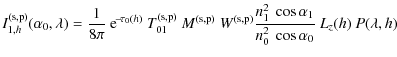
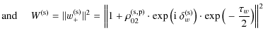
where
B.4.3 Radiant intensity observed in medium 1
Until now, we have not being interested in the wavelength dependence of the emission. The observed intensity depends on ![]() because each dipole radiates with a power
because each dipole radiates with a power
![]() that depends on the wavelength through an emission profile
that depends on the wavelength through an emission profile
![]() (in nm-1)
proper to the material of the film. In the case of photoluminescence,
the emission of each dipole will also result in an excitation absorbed
by the film (
(in nm-1)
proper to the material of the film. In the case of photoluminescence,
the emission of each dipole will also result in an excitation absorbed
by the film (
![]() is the power absorbed in unit of length (W.m-1)) that can depend on the film depth h. The emission also results in the photoluminescence yield
is the power absorbed in unit of length (W.m-1)) that can depend on the film depth h. The emission also results in the photoluminescence yield
![]()
![]() .
.
The specific power emitted by unit of film length (W nm-1 m-1) is
| (B.16) |
The total power (W) between the wavelengths
| |
= | 
|
(B.17) |
| = | 
|
(B.18) |
Moreover, because the whole film is radiating, the electric dipoles
|
(B.19) | ||
| (B.20) |
The total power between the wavelengths
|
(B.21) |
Appendix C: Fresnel coefficients
In this appendix, we express the Fresnel coefficients for an absorbing medium (meaning with a complex refractive index).
C.1 Reflection
The Fresnel reflection coefficients are given by the equations:
|
|
(C.1) |
The angles
| (C.2) |
The variables
C.2 Transmission
The Fresnel transmission coefficients (ratio of wave amplitudes) are given by the equations:

|
(C.3) |
| (C.4) |
The Fresnel transmittances (ratio of powers) are given by the equations
| |
= | 
|
(C.5) |
where Ai,j is the surface section of the light beam in medium i or j, and Pi,j and
| |
= | 
|
(C.6) |
| = | (C.7) |
Remark: In the same way, the reflectance is also defined as
| (C.8) |
We can also define another transmission factor
| |
= | (C.9) | |
| = | 
|
(C.10) | |
| = | 
|
(C.11) |
Current usage metrics show cumulative count of Article Views (full-text article views including HTML views, PDF and ePub downloads, according to the available data) and Abstracts Views on Vision4Press platform.
Data correspond to usage on the plateform after 2015. The current usage metrics is available 48-96 hours after online publication and is updated daily on week days.
Initial download of the metrics may take a while.