Non-thermal radio emission from O-type stars - IV. Cygnus OB2 No. 8A

Free Access

Issue		A&A Volume 519, September 2010


Article Number		A111
Number of page(s)		18
Section		Stellar atmospheres
DOI		https://doi.org/10.1051/0004-6361/200913450
Published online		21 September 2010

Online Material

Appendix A: Modelling

Most of the calculations discussed here are limited to the two-dimensional (2D) plane of the binary orbit. Only in Sect. A.7 do we rotate the results of the 2D calculations into the three-dimensional (3D) simulation volume that is used to calculate the resulting flux.

A.1 Binary orbit

Figure A.1 shows how the two stars are positioned in the XY plane of the 3D simulation volume. The primary is at the centre of the volume and the position of the secondary is determined by the orbital phase. The angle of periastron ( $\omega$ ) is measured from the intersection of the plane of the sky with the plane of the orbit. The sight-line towards the observer is in the YZ plane and the inclination angle i is the angle between the plane of the sky and the orbital plane. The secondary rotates clockwise in this figure (as seen from above). Periastron corresponds to phase 0.0.

$\begin{figure} \par\includegraphics[width=9cm,clip]{13450fg10.eps} \end{figure}$	Figure A.1: Binary orbit in the XY plane of the 3D simulation volume. The primary is positioned at the centre of the volume. The argument of periastron is denoted $\omega$ and the inclination angle i. The units on the axes are $R_{\odot }$ .
Open with DEXTER

A.2 Contact discontinuity

The position of the contact discontinuity at any given orbital phase is determined by the balance of ram pressure between the velocity components orthogonal to the contact discontinuity (see equations in Antokhin et al. 2004). These equations take into account that the terminal velocity of the winds may not have been reached yet before they collide. Specifically, in the Cyg OB2 No. 8A standard model presented in Sect. 5.1, the winds collide with $0.65 ~ \varv_\infty$ (primary) and $0.71 ~ \varv_\infty$ (secondary) at the apex at periastron. After the stellar wind material has passed through the shock, it then moves outward parallel to the contact discontinuity (there is also a small orthogonal velocity component, see Sect. A.5). We assume that the shocks and the contact discontinuity are sufficiently close to one another that we do not need to make a distinction in their geometric positions. On each side of the contact discontinuity, we assume the stellar wind to have a $\beta=1$ velocity law and a density derived from the mass conservation law, using the assumed velocity law and mass-loss rate.

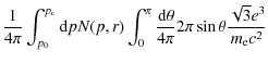
A.3 Momentum distribution relativistic electrons

We determine the momentum distribution of the relativistic electrons for a grid of points along the two shocks. We start with a population of electrons generated at a given point on the shock itself. We then follow the time evolution of this population as it advects away and cools down. The momentum distribution uses a grid that is uniform in $\log p$ , between p₀ = 1.0 MeV/c (for the choice of this specific value, see Van Loo et al. 2004) and the upper limit $p_{\rm c}$ (defined below, Eq. (A.3)) These limits are sufficiently wide to cover all of the radio emission we are interested in. We stop following the electrons when their momentum falls below p₀, or when they leave the simulation volume. (In our calculations we checked that the emission beyond the simulation volume is negligible.)

In the following, we refer mainly to Van Loo (2005, hereafter VL) as the source for the equations. Citations to the original papers can be found in that reference.

A.4 New relativistic electrons

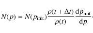
At the shock, new relativistic electrons are put into the system. Taking into account the particle acceleration mechanism and the inverse Compton cooling, it can be shown that their momenta follow a modified power-law distribution (VL, Eqs. (5.5), (5.6)):

N(p)	=	$\displaystyle N_{\rm E} p^{-n} \left(1 - \frac{p^2}{p_{\rm c}^2} \right)^{(n-3)/2} ,$	(A.1)
n	=	$\displaystyle \frac{\chi +2 }{\chi -1} \cdot$	(A.2)

With (VL, Eqs. (5.1)-(3)):

$\begin{displaymath}\left( \frac{p_{\rm c}}{m_{\rm e} c} \right)^2 = \frac{\chi ... ...i^2 - 1} \frac{4\pi r^2}{\sigma_{\rm T} L_*} \frac{eB(r)}{c} , \end{displaymath}$

(A.3)

with $m_{\rm e}$ and e the mass and charge of the electron, $\sigma_{\rm T}$ the Thomson electron scattering cross section, c the speed of light, L_* the luminosity of the star and r the distance of the point on the shock to the star. Because there are two stars, we should calculate the contribution of both:

$\begin{displaymath}\frac{L_*}{r^2} = \frac{L_{*,1}}{r_1^2} + \frac{L_{*,2}}{r_2^2} , \end{displaymath}$

(A.4)

with r₁ the distance to the primary and r₂ the distance to the secondary. Also (VL, Eq. (3.7)):

$\displaystyle \Delta u = u_1 - u_2 = u_1 \frac{\chi-1}{\chi} ,$

(A.5)

where u₁ is the upstream velocity and u₂ the downstream one and the shock strength $\chi=u_1/u_2$ . Throughout this work we assume strong shocks with $\chi=4$ , but we note that higher values can be expected in radiative shocks.

The normalization factor $N_{\rm E}$ is related to $\zeta$ , the fraction of energy that gets transferred from the shock to the relativistic particles, by (VL, Eq. (5.10)):

$\displaystyle N_{\rm E} = 4 \frac{\zeta}{\displaystyle \log_{\rm e} \left(\frac{p_{\rm c}}{p_0} \right)} \rho_1 \frac{\Delta u^2}{c} \quad ({\rm for}~\chi=4),$

(A.6)

where $\rho_1$ is the upstream density and we assume $\zeta=0.05$ (Blandford & Eichler 1987; Eichler & Usov 1993).

The magnetic field at distance r to the relevant star is assumed to be given by (Weber & Davis 1967; (VL, Eq. (2.48))):

$\begin{displaymath}B(r) = B_* \frac{\varv_{\rm rot}}{\varv_\infty} \frac{R_*}{r} , \end{displaymath}$

(A.7)

where B_* is the surface magnetic field (assumed to be 100 G) and $\varv_{\rm rot}$ is the equatorial rotational velocity. This equation is only valid at larger distances from the star, but we use it everywhere as the region close to the star will not be visible anyway (due to free-free absorption). This equation neglects any amplification of the field (such as described by, e.g. Bell 2004) or any reduction by magnetic reconnection. For each of the two shocks, the corresponding magnetic field is taken into account.

A.5 Advection and cooling

During a time step $\Delta t$ , the relativistic electrons advect away and cool mainly due to inverse Compton and adiabatic cooling (see Chen 1992; and VL, p. 96, for a discussion on other cooling mechanisms and why they are not important in the present situation).

The equation for cooling of a single relativistic electron can be written as:

$\displaystyle \frac{{\rm d}p}{{\rm d}t}$	=	$\displaystyle -a p^2 +b p \quad\mbox{with}$	(A.8)
a	=	$\displaystyle \frac{\sigma_{\rm T}}{3 \pi m_{\rm e}^2 c^3} \frac{L_*}{r^2} ,$	(A.9)
b	=	$\displaystyle \frac{1}{3 \rho} \frac{\Delta \rho}{\Delta t},$	(A.10)

where a p² gives the inverse Compton cooling (VL, Eq. (5.2)) and b p the adiabatic cooling (which can be derived from the fact that for adiabatic cooling $p \propto T^{1/2} \propto \rho^{(\gamma-1)/2}$ and using $\gamma=5/3$ ).

Integration of Eq. (A.8) gives:

$\begin{displaymath}p = \frac{p_{\rm init} \exp (b \Delta t)}{\displaystyle 1 - \frac{a}{b} p_{\rm init} \left( 1 - \exp (b \Delta t) \right)} , \end{displaymath}$

(A.11)

where $p_{\rm init}$ is the momentum at the previous time step. We can invert this to:

$\begin{displaymath}p_{\rm init} = \frac{p \exp (-b \Delta t)}{\displaystyle 1 - \frac{a}{b} p \left( 1 -\exp (-b \Delta t) \right)} \cdot \end{displaymath}$

(A.12)

We will also need the following derivative:

$\begin{displaymath}\frac{{\rm d}p_{\rm init}}{{\rm d}p} = \frac{\exp (-b \Delta ... ...{a}{b} p \left( 1 - \exp (-b \Delta t) \right)\right]^2} \cdot \end{displaymath}$

(A.13)

We assume that only the momentum p changes significantly with time; for the other variables, we take their value mid-way between the start and the end of the time step $\Delta t$ . The density $\rho$ we need in Eq. (A.10) is the one between the shock and the contact discontinuity. We do not have detailed hydrodynamical models for this, so we simply approximate it by $\rho = \chi \rho_{\rm s}$ where $\rho_{\rm s}$ is the density in the smooth wind at the position of the shock. We stress once again that in these radiative shocks, the post-shock density increases rapidly downstream, maybe by several orders of magnitude, rather than the $\chi=4$ value we use.

The above equations describe what happens to a single relativistic electron. The time evolution of the momentum distribution function over the time step $\Delta t$ is:

$\begin{displaymath}N(p) = N(p_{\rm init}) \frac{\rho (t+\Delta t)}{\rho (t)} \frac{{\rm d}p_{\rm init}}{{\rm d}p} \cdot \end{displaymath}$

(A.14)

We stop following the electrons when their momentum falls below p₀, or when they leave the simulation volume.

In our simplifying assumptions the contact discontinuity and the shock are at the same geometrical position. Taken literally, this would result in a synchrotron emitting region that has zero thickness and zero synchrotron emission. In the true hydrodynamical situation, particles move through the shock (which is at some distance from the contact discontinuity) and then move slowly towards the contact discontinuity. At the same time, they are being advected outward with a velocity parallel to the contact discontinuity that is much larger than the corresponding orthogonal velocity. The thickness of the synchrotron emitting region is set by the combination of these two velocities. In the absence of hydrodynamical information, we use the following procedure to determine these velocities. The parallel component ( $\varv_{\Vert}$ ) at the contact discontinuity is determined by projecting the smooth wind velocity vector on to the contact discontinuity. At other positions in the wind, we interpolate in the grid of $\varv_{\Vert}$ as a function of the y-coordinate. The orthogonal component ( $\varv_{\bot}$ ) at the contact discontinuity is expected to be of the order of the orthogonal component of the material coming into the shock, with a minimum value corresponding to the thermal expansion of the gas. As a simplification, we set it exactly equal to the incoming orthogonal component, and we use the same type of interpolation as for the parallel velocity to determine it at other positions. We reverse the orthogonal velocity direction to have the gas moving away from the contact discontinuity. Note that this situation is ``inside out'' compared to the true hydrodynamical situation where the particles move towards the contact discontinuity. The thickness of the synchrotron emitting region is so small however that this inversion has negligible influence on our results.

A.6 Emissivity

The equation for the emissivity is given by (VL, Eq. (B.1)):

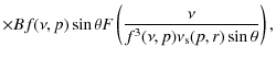
$\displaystyle j_\nu(r)$	=	$\displaystyle \frac{1}{4 \pi} \int_{p_0}^{p_{\rm c}} {\rm d}p N(p,r) \int_0^\pi \frac{{\rm d}\theta}{4\pi} 2\pi \sin \theta \frac{\sqrt{3} e^3}{m_{\rm e} c^2}$
		$\displaystyle \times B f(\nu,p) \sin \theta F \left(\frac{\nu}{f^3(\nu,p)\nu_{\rm s}(p,r) \sin\theta} \right) ,$	(A.15)

with (VL, Eq. (2.51), (2.50)):

$\displaystyle f (\nu,p)$	=	$\displaystyle \left[ 1+ \frac{\nu_0^2}{\nu^2} \left( \frac{p}{m_{\rm e} c} \right)^2 \right]^{-1/2}$	(A.16)
$\displaystyle \nu_0$	=	$\displaystyle \sqrt{\frac{n_{\rm e} e^2}{\pi m_{\rm e}}}$	(A.17)
$\displaystyle \nu_{\rm s} (p,r)$	=	$\displaystyle \frac{3}{4 \pi} \frac{eB}{m_{\rm e} c} \left( \frac{p}{m_{\rm e} c} \right)^2$	(A.18)
F(x)	=	$\displaystyle \int_x^\infty {\rm d}\eta K_{5/3} (\eta) .$	(A.19)

We use Eq. (A.7) for the magnetic field. Note that this is an approximation, as the shock may compress the magnetic field as well, leading to higher values than given by Eq. (A.7). The expression for $j_\nu (r)$ is evaluated at position r and frequency $\nu$ . The f function corrects for the Razin effect and K_5/3 is the modified Bessel function. To calculate $n_{\rm e}$ , the number density of the thermal electrons (i.e. those in the non-relativistic plasma), we use:

$\begin{displaymath}n_{\rm e}=\frac{\chi \rho_{\rm s}}{m_{\rm H}} \frac{1.2}{1.4} , \end{displaymath}$

(A.20)

where $\rho_{\rm s}$ is the smooth wind density and $m_{\rm H}$ the mass of a hydrogen atom. The factor 1.2/1.4 takes into account a fully ionized hydrogen+helium solar composition. In these radiative shocks the post-shock density may increase by several orders of magnitude rather than by $\chi=4$ , which will influence the value of $n_{\rm e}$ .

To reduce the computing time we set $\sin \theta =1$ in the $f \sin \theta$ factors of Eq. (A.15) and we also use:

$\begin{displaymath}\int_0^\pi \frac{{\rm d}\theta}{4\pi} {2\pi \sin \theta} = 1 . \end{displaymath}$

(A.21)

The F function is precalculated on a grid of x-values; the evaluation of the function then reduces to an interpolation.

A.7 Map into 3D grid

Using the equations from the previous sections, we can make a 2D map of the synchrotron emission (part of which is shown in Fig. 6). Note that the synchrotron emission extends on both sides of the contact discontinuity, because there is a shock on either side. Based on the cylindrical symmetry around the line connecting the two stars (at the given orbital phase), we then ``rotate'' this 2D map into the 3D simulation volume.

It is important that during this procedure we do not lose part of the emission due to interpolation or reduced resolution. To achieve this, we use volume-integrated emissivities. While doing the 2D calculation we store the volume integrated emissivity $\overline{j_\nu(r)}$ defined by:

$\begin{displaymath}\overline{j_\nu(r)} \Delta V = \int_{\Delta V} j_\nu(r) {\rm d} V . \end{displaymath}$

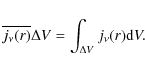
(A.22)

The volume $\Delta V$ used in this definition is determined as follows. We consider the 2D surface covered by (1) the step in the coordinate along the contact discontinuity and (2) the distance travelled by the relativistic electrons between two consecutive time steps. We then rotate this surface around the line connecting the two stars over a small angle $\alpha$ , thereby defining the emissivity volume $\Delta V$ .

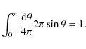
When we have finished the full 2D calculation, we rotate the 2D plane into the 3D simulation volume, using steps of angle $\alpha$ (as defined above). For each of the emissivity volumes $\Delta V$ defined above, and for a given rotation angle, we determine what fraction of the rotated volume overlaps with the cells in the 3D simulation volume. This is done by subdividing each dimension of the $\Delta V$ volume into three. For each of the resulting 3³ points we determine in which 3D simulation cell they end up after rotation. A running sum for that cell is then updated with the fraction 3^-3 of the volume integrated emissivity $\overline{j_\nu}$ of the rotated volume. At the end of this procedure, the accumulated emission in each 3D simulation cell is divided by its volume, thus obtaining $j_\nu$ for that cell.

In this procedure we lose some resolution, specifically around the apex, where the 2D resolution is quite high but where the 3D resolution is much lower. However, because of the use of volume-integrated quantities, we do not lose any of the synchrotron emission. Furthermore, the apex of the wind is well hidden by the free-free absorption and will therefore not contribute to the resulting radio flux at the wavelengths we consider. If our model were to be applied to X-rays, optical emission or radio emission at much shorter wavelengths, a higher-resolution 3D grid would be required.

In the 3D model. we also include the thermal free-free opacity and emissivity, which is due to the ionized wind material. To calculate these we use the Wright & Barlow (1975) equations. The winds of both stars are assumed to be smooth. For the Gaunt factor at frequency $\nu$ we use the equation from Leitherer & Robert (1991):

$\begin{displaymath}g_\nu = 9.77 \left( 1 + 0.13 \log_{10} \frac{T_{\rm e}^{3/2}}{Z \nu} \right), \end{displaymath}$

(A.23)

where $T_{\rm e}$ is the thermal electron temperature in the wind and Z the charge of the ions. The stars themselves are introduced into the simulation volume as high opacity spheres. We then solve the radiative transfer equation in Cartesian coordinates along the line of sight. We use Adam's (Adam 1990) finite volume method because of its simplicity. By repeating the whole procedure for a number of orbital phases and wavelengths, we calculate the radio light curve at these wavelengths and determine how the fluxes and spectral index change with phase.

Appendix B: Data reduction

The data reduction is accomplished using the Astronomical Image Processing System (AIPS), developed by the NRAO. We follow the standard procedures of antenna gain calibration, absolute flux calibration, imaging and deconvolution. Where possible, we apply self-calibration to the observations (see notes to Table B.1). We measure the fluxes and error bars by fitting elliptical Gaussians to the sources on the images. The error bars listed in Table B.1 include not only the rms noise in the map, but also an estimate of the systematic errors that were evaluated using a jackknife technique. This technique drops part of the observed data and redetermines the fluxes, giving some indication of systematic errors that can be present. Upper limits are three times the uncertainty as derived above. For details of the reduction, we refer to the previous papers in this series (Blomme et al. 2007; Van Loo et al. 2008; Blomme et al. 2005). We exclude from Table B.1 those observations with upper limits higher than 6 mJy (which corresponds to about 3 times the highest detection at all wavelengths).

A comparison with values previously published in the literature shows that in most cases the error bars overlap with ours. There are just a few exceptions, which we discuss further. Bieging et al. (1989) list only an upper limit for the AC116 2 cm observation, while we find a detection (though marginal at just above 3 sigma). Our detection is quite consistent in all variants we consider in the jackknife test and is at the exact position of Cyg OB2 No. 8A, so we consider it a detection. For the AS483 6 cm, Waldron et al. (1998) find a value of $1.04 \pm 0.08$ mJy, which is $\sim$ 20% lower than our value. A possible explanation is that they did not correct for the decreasing sensitivity of the primary beam. This effect is important when the target is not in the centre of the image, and is approximately 20% for the position of No. 8A on the image. Puls et al. (2006) list an upper limit of 0.54 mJy for the AS786 6 cm observation, but we clearly detect Cyg OB2 No. 8A on the image we made. Bieging et al. (1989) find a slightly lower value of $1.0 \pm 0.1$ mJy for the AC116 1984-12-21, 20 cm observation. We have no explanation for these last two discrepancies.

We also take the opportunity to correct some clerical errors in the literature: Bieging et al. (1989) date the CHUR observations as 1980-Mar-22, but it should be 1980-May-23. The Waldron et al. (1998) 1991 observation was made at 3.6 cm, not at 6 cm and the 1992 observation was made in January, not June.

Table B.1: Reduction of the Cyg OB2 No. 8A VLA data.

Current usage metrics show cumulative count of Article Views (full-text article views including HTML views, PDF and ePub downloads, according to the available data) and Abstracts Views on Vision4Press platform.

Data correspond to usage on the plateform after 2015. The current usage metrics is available 48-96 hours after online publication and is updated daily on week days.

Initial download of the metrics may take a while.