


| Issue |
A&A
Volume 711, July 2026
|
|
|---|---|---|
| Article Number | A99 | |
| Number of page(s) | 17 | |
| Section | Astronomical instrumentation | |
| DOI | https://doi.org/10.1051/0004-6361/202558701 | |
| Published online | 07 July 2026 | |
Characterization of telecentric dual-etalon Fabry-Pérot systems from observational data
Properties of the CRISP2 instrument at the Swedish 1-m Solar Telescope
Institute for Solar Physics, Dept. of Astronomy, Stockholm University, AlbaNova University Centre,
106 91
Stockholm,
Sweden
★ Corresponding author: This email address is being protected from spambots. You need JavaScript enabled to view it.
Received:
19
December
2025
Accepted:
5
May
2026
Abstract
Context. Fabry-Pérot interferometer (FPI) observations are commonly used in solar physics to infer physical parameters in the photosphere and chromosphere using observational modeling. Such techniques require detailed knowledge of the spectral instrumental profile to produce accurate results.
Aims. We present a method to characterize the spatial variation of the parameters of dual-etalon FPI instruments mounted in a telecentric configuration: spatially resolved cavity separation, the reflectivities of both etalons, and the prefilter variation across the field of view. We aim to characterize the field-of-view dependence of the parameters of the new CRISP2 FPI.
Methods. We implemented a forward model of the FPI instrumental degradation combined with a template average quiet-Sun spectrum at disk center to model two sets of observational data. Our method does not require any changes to the optical setup or the use of external illumination sources. We assessed the validity of several functional forms to calculate the FPI transmission profiles.
Results. Our results show that, in general, including the secondary transmission peaks at ±1 times the free spectral range (FSR) and a detailed estimate of the prefilter curve are necessary to obtain accurate values of both etalon reflectivities. For very narrow prefilters relative to the FSR, the former requirement can be relaxed. Our results show that the CRISP2 cavity separation is very flat, with an RMS variation below 2 nm over the entire field of view for both etalons. Reflectivity RMS variations are 0.4 and 0.3% for the primary and secondary etalons at 617.3 nm.
Conclusions. We assessed the data and modeling requirements needed to derive accurate dual-etalon telecentric FPI parameters and minimize errors in determining etalon reflectivities. The methods described in this paper are relevant for the characterization of present and future FPI instruments, and we have made them publicly available to the solar community.
Key words: instrumentation: interferometers / methods: data analysis / techniques: imaging spectroscopy
© The Authors 2026
 Open Access article, published by EDP Sciences, under the terms of the Creative Commons Attribution License (https://creativecommons.org/licenses/by/4.0), which permits unrestricted use, distribution, and reproduction in any medium, provided the original work is properly cited.
This article is published in open access under the Subscribe to Open model. This email address is being protected from spambots. You need JavaScript enabled to view it. to support open access publication.
1 Introduction
The use of Fabry-Pérot interferometers (FPIs) in imaging polarimeters has become increasingly popular in observational solar physics during the past two decades. These instruments allow very narrow-band imaging (R = λ/δλ ≈ 50 000–120 000) and can reconstruct a spectral line profile in each pixel of the field of view (FOV) by sequentially scanning through the wavelengths of the profile. Their main advantages are that they allow for a large FOV (e.g., Scharmer et al. 2026), that image reconstruction techniques can be easily applied to FPI observations (van Noort et al. 2005), and that a polarizing beam splitter, needed for polarimetric measurements, can be mounted close to the science cameras.
Arguably, their main limitation is the limited amount of time that can be spent on the spectral scan before the solar scene changes between the different wavelength positions of the scan. This limitation is largely influenced by the spatial resolution of the system, and on the characteristic evolution time of the layer of the solar atmosphere under study. For example, the scanning time for chromospheric observations acquired with a 1-m solar telescope (with a critical sampling of 47 km px−1 at 617.3 nm) can be dominated by the Alfvén speed (~100 km s−1) or by the sound speed (~10 km s−1), which effectively limits the available time to acquire a line scan to ≲1–10 s (van Noort & Rouppe van der Voort 2006; Felipe et al. 2018; Schlichenmaier et al. 2023; Rouppe van der Voort et al. 2023). At lower spatial resolution this requirement is less constrained by fast dynamics in the solar atmosphere, allowing longer scan times. The scan time can be spent at a few line positions with long exposure times or at many positions with shorter exposure times. Examples of modern FPIs are the Interferometric BIdimensional Spectrometer (IBIS, Cavallini 2006), the Crisp Imaging Spectropolarimeter (CRISP, Scharmer 2006; Scharmer et al. 2026), the Visible Tunable Filter (VTF, Schubert et al. 2017), the Polarimetric and Helioseismic Imager (PHI, Solanki et al. 2020), and the Tunable Magnetograph (TuMag, del Toro Iniesta et al. 2025).
FPIs provide one of the best alternatives for photospheric and chromospheric studies that require a large FOV and relatively high cadence. To model FPI datasets, usually using data inversion techniques (del Toro Iniesta & Ruiz Cobo 2016) requires an accurate estimate of the instrumental spectral transmission profile (hereafter, transmission profile) to make a meaningful comparison between synthetic spectra from simulations or inversion methods and observations. Etalons mounted in a telecentric configuration exhibit unavoidable instrumental effects, including field-dependent (random) wavelength shifts and variations in the FWHM of the transmission profile. These effects can be calibrated to produce a FOV-dependent spectral transmission profile, which should be included in the inversion process.
A recent series of papers (Bailén et al. 2019a; Bailén et al. 2019b; Bailén et al. 2020; Bailén et al. 2021) has derived analytical expressions for the characterization of single-etalon systems. These expressions allow for a very fast determination of an etalon’s instrumental profile. However, the validity of the analytical expressions is restricted to cases where the etalon is not tilted, which is a crucial aspect of dual-etalon systems for removing inter-etalon reflections.
We describe an FPI characterization method for telecentric dual-etalon systems (comprising one prefilter and two etalons) using observational datasets. The techniques described in this paper build upon previous studies (Scharmer 2006; de la Cruz Rodríguez 2010; Bailén et al. 2019a; Santamarina Guerrero et al. 2024) and on many years of experience at the Swedish 1-m Solar Telescope (SST). Similar techniques have also been used in the characterization of FPI instruments of collimated configurations (Reardon & Cavallini 2008). We extend previous studies by including a model that can deal with the symmetry-breaking effects of a tilted etalon, a full characterization of the order-suppressing etalon, and an assessment of the importance of accurate prefilter modeling.
We use these methods to analyze the performance of the new CRISP2 FPI (Scharmer et al. 2026) mounted at the SST Scharmer et al. 2003 at 617.3 nm. The CRISP2 instrument is an evolution of CRISP (Scharmer 2006), optimized for a larger FOV.
2 The CRISP2 FPI system
The design concept of CRISP2 (Scharmer et al. 2026) is identical to that of CRISP: it consists of two etalons mounted in a telecentric configuration and with the same cavity separation ratio as CRISP. However, CRISP2 is optimized for a larger FOV (Dfov ≈ 120″) than CRISP by using larger etalons and a lower F-ratio (F/140) at the etalons. A high-spectral-resolution etalon (hereafter HRE), with a narrow passband, sets the wavelength of the observation. A second etalon with a carefully chosen and different free-spectral range (the spectral distance between consecutive transmission peaks) effectively suppresses secondary transmission peaks and leaves only the main transmission peak at the desired wavelength (see Fig. 1). To mitigate the negative effects of the lower F-ratio, the high-resolution etalon of CRISP2 has a slightly lower reflectivity (93%) than that of CRISP (94%).
Scharmer (2006) proposed using a low-resolution secondary etalon (LRE) with a lower reflectivity than the primary etalon. The lower reflectivity widens its transmission profile, which strongly reduces the effect of mismatched profiles between the two etalons caused by random errors in their cavity separations. This simple approach maintains high system transmission while minimizing variations in the shape of the transmission profile across the FOV. An order-selecting prefilter is placed before the etalons to suppress light outside the spectral window under consideration and to reduce contribution from secondary transmission peaks. Tilting the LRE and placing a pupil stop at the location of the pupil image in front of the camera lens eliminates internal reflections between the two etalons. Consequently, this design completely eliminates phase error terms from inter-etalon reflections.
The nominal cavity separations of the two etalons are ![Mathematical equation: $\[C_{\text {HRE}}^{0}= 787 ~\mu \mathrm{m}\]$](/articles/aa/full_html/2026/07/aa58701-25/aa58701-25-eq1.png) and
and ![Mathematical equation: $\[C_{\text {LRE}}^{0}=300 ~\mu \mathrm{m}\]$](/articles/aa/full_html/2026/07/aa58701-25/aa58701-25-eq2.png) , resulting in a cavity separation ratio (co-tuning factor) of
, resulting in a cavity separation ratio (co-tuning factor) of ![Mathematical equation: $\[r_{c}=C_{\mathrm{LRE}}^{0} / C_{\mathrm{HRE}}^{0}=0.38119\]$](/articles/aa/full_html/2026/07/aa58701-25/aa58701-25-eq3.png) . Our measured co-tuning factor is very similar, rc = 0.38273. Fig. 2 illustrates the factory-measured reflectivities of the two etalons and the resulting full width at half maximum (FWHM) of the transmission profile as a function of wavelength. Table 1 lists spectral lines that have been or could be observed with CRISP2, together with the corresponding reflectivities and transmission-profile FWHM.
. Our measured co-tuning factor is very similar, rc = 0.38273. Fig. 2 illustrates the factory-measured reflectivities of the two etalons and the resulting full width at half maximum (FWHM) of the transmission profile as a function of wavelength. Table 1 lists spectral lines that have been or could be observed with CRISP2, together with the corresponding reflectivities and transmission-profile FWHM.
To make use of the full potential FOV of CRISP2, we used 50-mm diameter filters (clear aperture >40 mm). At the time of writing, we had only two of these larger prefilters, designed for H-α 656.3 nm and CaII 854.25 nm, while a filter for FeI 617.33 nm was still in development. The filter analyzed in detail in this paper is a smaller prefilter for CRISP (32 mm diameter, 26.5 mm clear aperture), which produces only a small FOV reduction compared to the 50-mm filters because the FOV is currently limited by the polarimetric modulator reused from CRISP. After the etalons, a polarizing beam splitter separates the light into two beams with orthogonal polarization states, which are recorded by two cameras (Ximea CB262RG-GP-X8G3). The resulting image scale in the camera focal plane is ![Mathematical equation: $\[0^{\prime\prime}_\cdot 05 / \mathrm{px}\]$](/articles/aa/full_html/2026/07/aa58701-25/aa58701-25-eq4.png) .
.
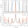 |
Fig. 1 Transmission profile at 617.3 nm measured with CRISP2. Top: high-resolution etalon (HRE), low-resolution etalon (LRE) and full transmission profiles, with the prefilter shape also indicated. Bottom: transmission profile and the same profile multiplied by the prefilter transmission, illustrating the attenuation of secondary lobes by the prefilter. |
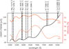 |
Fig. 2 Factory-measured reflectivities of the etalons (red) and the corresponding instrumental profile full width at half maximum (FWHM) for the CRISP2 instrument (black). The solid red line depicts the reflectivity of the high-resolution etalon, whereas the dashed red line corresponds to the reflectivity of the low-resolution etalon. We calculated the FWHM of the profile assuming perfect co-tuning of the profiles from the two etalons and the factory nominal reflectivities. |
Reflectivities of CRISP2 etalons and transmission-profile FWHM.
3 Characterization of the CRISP2 FPI system from observational datasets
3.1 The CRISP2 transmission profile
Assuming that there is no absorption by the coatings, the theoretical electric-field transmission profile of an etalon for a ray with incidence angle θ relative to the normal is (see, e.g., Hecht 2017; Born & Wolf 2019)
![Mathematical equation: $\[\begin{aligned}T(R, C, \theta, \lambda) & =\left(\frac{1-R}{1-R \mathrm{e}^{i \psi}}\right) \mathrm{e}^{i \psi / 2} \\& =\frac{1}{1-R}\left(\frac{(1-R) ~\cos (\psi / 2)+i(1+R) \sin (\psi / 2)}{1+F ~\sin ^2(\psi / 2)}\right),\end{aligned}\]$](/articles/aa/full_html/2026/07/aa58701-25/aa58701-25-eq5.png) (1)
(1)
where ψ = 4πn cos(θ)C/λ, R is the reflectivity (intensity reflectance) of the etalon, C is the cavity separation, n is the refractive index of the cavity (n = 1 in our case), F = 4R/(1 − R)2, and λ is the wavelength. Bailén et al. (2019a) recently noted the factor eiψ/2, which is commonly ignored in the literature. It is a global phase factor that originates from the propagation of the first ray that enters the cavity before it is reflected at the second surface. This term has no influence on collimated beams, but it carries a phase difference between rays with different incidence angles. Although this phase term is very small compared to the net phase error accumulated over many reflections inside the cavity, it should be included in the calculations.
As the FPI scans over a spectral line, both etalons are cotuned to the same wavelength positions. Assuming that there are no internal reflections between the two etalons, which are suppressed here by the LRE tilt and the pupil stop, the effective transmission profile at each wavelength is therefore the product of the transmission profiles from each etalon (see e.g., von der Lühe & Kentischer 2000):
![Mathematical equation: $\[T\left(R_h, C_h, R_l, C_l, \theta, \lambda\right)=T\left(R_l, C_l, \theta, \lambda\right) \cdot T\left(R_h, C_h, \theta, \lambda\right),\]$](/articles/aa/full_html/2026/07/aa58701-25/aa58701-25-eq6.png) (2)
(2)
where the h and l subscripts correspond to high- and low-resolution etalon parameters, respectively.
A rough simplification is to assume perpendicular incidence with the surface of the etalon, for which we only need to consider the transmission profile along one incidence angle. This simplification reasonably approximates the real transmission profile when the range of incidence angles of the telecentric beam is very small, which can be obtained when the F-ratio multiplied by the refractive index of the cavity, if different from that of air, is large. Because non-perpendicular rays decrease the cos(θ) term, the profile shifts toward shorter wavelengths. In reality, the beam converges slowly (F/140 for CRISP2 and F/165 for CRISP), resulting in incidence angles in the range [0, 1/(2F)] (pupil apodization).
A better approximation of the real transmission profile is obtained by including pupil-apodization effects through a weighted integral over all incidence angles of the telecentric beam (in this case defining an integration quadrature of Nray incidence angles), while assuming axial symmetry around the optical axis. To simplify the notation, we omit the wavelength dependence of the profile, and the angular integral can then be expressed as
![Mathematical equation: $\[T\left(R_h, C_h, R_l, C_l\right)=\sum_{i=0}^{N_{\mathrm{ray}}-1} w_i \mathrm{e}^{-i k_4 \phi_4}\left\{T\left(R_l, C_l, \theta_i\right) \cdot T\left(R_h, C_h, \theta_i\right)\right\},\]$](/articles/aa/full_html/2026/07/aa58701-25/aa58701-25-eq7.png) (3)
(3)
where wi are normalized integration weights (∑i wi = 1). The e−ik4ϕ4 factor is a focus term that we discuss in Sect. 3.2.
Since θ is a radial coordinate, evenly spaced θi are associated with an annular area proportional to θi, which must be accounted for in the weights wi ∝ 2πθiΔθ. However, we can place the rays at angles θi such that ![Mathematical equation: $\[\theta_{i}^{2}\]$](/articles/aa/full_html/2026/07/aa58701-25/aa58701-25-eq8.png) are evenly distributed in
are evenly distributed in ![Mathematical equation: $\[\left[0, \theta_{\text {max }}^{2}=1 /(2 F)^{2}\right]\]$](/articles/aa/full_html/2026/07/aa58701-25/aa58701-25-eq9.png) and then take the square-root of the result,
and then take the square-root of the result,
![Mathematical equation: $\[\theta_i=\sqrt{\frac{1}{(2 F)^2} \frac{i}{N_{\mathrm{ray}}-1}},\]$](/articles/aa/full_html/2026/07/aa58701-25/aa58701-25-eq10.png) (4)
(4)
where i is the ray number, taking values in the range [0, Nray − 1]. In this case, the larger contribution from external rings is included in the ray distribution, so that all rays can now have the same weight. We note that, for inclined rays, the transmission profile shifts towards shorter wavelengths, and therefore the integrated profile from Eq. (3) also slightly shifts compared to perpendicular incidence for an identical cavity separation. The effective shift of the profile can easily be estimated as
![Mathematical equation: $\[\Delta \lambda_{\text {peak }}=\left(\sum_{i=0}^{N_{\mathrm{ray}}-1} w_i \lambda_0 \cos \theta_i\right)-\lambda_0,\]$](/articles/aa/full_html/2026/07/aa58701-25/aa58701-25-eq11.png) (5)
(5)
where λ0 is the wavelength at which the peak of the perpendicularly incident ray is centered at (λ0 is such that C = mλ0/2, where m is an integer). Another effect of the angular integral is that the resulting profile becomes slightly asymmetric.
The approximation just discussed, which we label conv (for converging), requires only Nray ≳ 7 to achieve a sufficiently accurate angular integral. The drawback of this model is that it neglects potential etalon tilts used to minimize internal reflections. For example, in CRISP and CRISP2, the LRE is tilted by 0.5/F, inducing an asymmetry in the integrated LRE transmission profile and a slightly lower transmission.
To include the effect of tilting the LRE etalon, the tilt angle on one axis must be added to the ray angles in the converging beam. This etalon tilt breaks the angular symmetry, making the problem more challenging. Figure 3 illustrates the angular distribution across the pupil for untilted and tilted etalons. Although some symmetry remains in the tilted case that could be exploited to define an analytical integration quadrature, we find it easier to simply calculate a 2D histogram over the angular distributions of the two etalons and use the central values of the bins as the inclination angles of the different rays. We illustrate these histograms in the bottom panels of Fig. 3, computed using 19 (left) and 7 (right) bins. In our tests, using Nray ≥ 7 per etalon yields a sufficiently accurate integration, with a maximum error below 0.5% relative to a calculation using 101 rays. The weight for each bin is given by the histogram value at that location. In the following, we refer to this case as the full calculation. The LRE tilt makes its profile more asymmetric than in the untilted case, and this asymmetry propagates to the total transmission profile, most notably in the wings.
Once the inclination angles and their weights are defined, the effective transmission profile can be obtained with an expression similar to Eq. (3), although the angles are defined separately for each etalon and all permutations must be evaluated in the integral with the corresponding weights. The intensity transmission profile is calculated as
![Mathematical equation: $\[\hat{T}=T \cdot T^{\dagger},\]$](/articles/aa/full_html/2026/07/aa58701-25/aa58701-25-eq12.png) (6)
(6)
where T† is the complex conjugate of T. When phase errors are small, the resulting transmission profile obtained using Eqs. (1), (3) and (6) is similar to that obtained by integrating individual intensity transmission profiles, although this is not strictly correct mathematically since
![Mathematical equation: $\[\sum_i\left(T \cdot T^{\dagger}\right) \neq\left(\sum_i T\right) \cdot\left(\sum_i T\right)^{\dagger}.\]$](/articles/aa/full_html/2026/07/aa58701-25/aa58701-25-eq13.png) (7)
(7)
In this study, we express the cavity separation errors of the LRE (ΔCLRE) relative to those of the HRE as
![Mathematical equation: $\[\begin{aligned}C_{\mathrm{HRE}}(x, y) & =C_{\mathrm{HRE}}^0+\Delta C_{\mathrm{HRE}}(x, y) \\C_{\mathrm{LRE}}(x, y) & =C_{\mathrm{LRE}}^0+\Delta C_{\mathrm{LRE}}(x, y)+\Delta C_{\mathrm{HRE}}(x, y) \cdot r_c,\end{aligned}\]$](/articles/aa/full_html/2026/07/aa58701-25/aa58701-25-eq14.png)
where CHRE and CLRE are the FOV-dependent cavity separations. In this way, the LRE is always co-tuned with the HRE unless ΔCLRE ≠ 0. As a result, the LRE cavity error map does not need to be corrected for HRE cavity errors after fitting.
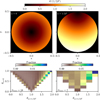 |
Fig. 3 Distribution of inclination angles across the (circular) pupil for a non-tilted case (α = 0, top left) and a tilt of α = 1/2F in the y axis (top right). Bottom panels: 2D histograms correlating the angles of the two cases (left: Nrays = 19, right: Nrays = 7). The histograms provide the integration weights used to perform the angular integral of the transmission profile over the pupil angles. |
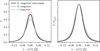 |
Fig. 4 Transmission profiles of the CRISP2 instrument calculated including instrument refocus (black), no refocus (blue), and by performing the angular integral directly on the intensity transmission profiles (dashed red). The profiles in the right panel are peak normalized. |
3.2 System optimization by refocusing
Scharmer (2006) performed an extensive analysis of the phase-error amplification function. This function has a quadratic dependence across the pupil, mimicking a defocus term. However, it also varies in strength across the transmission profile. Therefore, optimal refocusing reduces, but cannot eliminate, these phase errors in the system. Although the analysis was described mainly in the context of improving image quality, refocusing also improves the overall transmission of the instrument.
The refocusing term can be modeled using a defocus Zernike term e−ik4ϕ4, where k4 is a constant that captures the amount of defocus, ![Mathematical equation: $\[\phi_{4}=\sqrt{3}(2 r-1)\]$](/articles/aa/full_html/2026/07/aa58701-25/aa58701-25-eq15.png) , and r is the normalized radius in the pupil for a given ray. The constant k4 can be optimized once to achieve maximum transmission. In practice, this term is automatically accounted for when the instrument is focused on the optical table.
, and r is the normalized radius in the pupil for a given ray. The constant k4 can be optimized once to achieve maximum transmission. In practice, this term is automatically accounted for when the instrument is focused on the optical table.
Figure 4 shows a comparison of profiles calculated with and without the refocusing term, and one profile calculated by direct integration of the intensity transmission profile (ignoring phase errors). Without refocusing (blue curve), the peak transmission is very low (76% of the phase-error-free case shown in dashed red) and the profile is wider. With the refocusing term, the transmission reaches 92% of that value and the resulting profile is only slightly narrower. We suspect that this difference is due to the approximation introduced in Eq. (7) for the integration of the intensity transmission profile.
Modern computers efficiently handle complex-number operations, and our implementation of the electric-field transmission-profile angular integral is only ~50–60% slower than computing the intensity transmission profile using real numbers.
3.3 The prefilter transmission curve
The prefilter curve can be modeled using an analytical formula,
![Mathematical equation: $\[P(\lambda)=\frac{p_{\mathrm{g}}}{1+\left(2 \frac{\lambda-p_{w_0}}{p_{\text {fwhm }}}\right)^{2 p_{\text {ncav }}}}\left\{1+w_{\text {apod }}\left(p_0 \Delta \lambda+p_1 \Delta \lambda^2+p_2 \Delta \lambda^3\right)\right\},\]$](/articles/aa/full_html/2026/07/aa58701-25/aa58701-25-eq16.png) (8)
(8)
where pg is a gain factor, pw0 is the central wavelength of the prefilter, pfwhm is the prefilter FWHM, pncav is the number of cavities of the prefilter, Δλ = λ − pw0, and p0, p1 and p2 are the coefficients of a polynomial used to account for deviations from the analytical shape of the prefilter, including asymmetries and spatial movement of fringes with wavelength. Schnerr et al. (2011) and de la Cruz Rodríguez et al. (2015) used similar expressions to describe the shape of interference prefilters, but in our case, we define the polynomial component relative to the prefilter central wavelength, ensuring a shift-invariant prefilter shape. We also introduce an apodization window (in the spectral dimension) that multiplies the polynomial component (wapod) to avoid negative values in the far wings of the prefilter. We define the apodization window relative to the central wavelength and FWHM of the prefilter:
![Mathematical equation: $\[w_{\text {apod }}=\frac{1}{4}\left\{\left(1+\tan~ h\left(\Delta \lambda_1\right)\right) \cdot\left(1-\tan~ h\left(\Delta \lambda_2\right)\right)\right\},\]$](/articles/aa/full_html/2026/07/aa58701-25/aa58701-25-eq17.png) (9)
(9)
where
![Mathematical equation: $\[\Delta \lambda_1=\frac{\pi}{2}\left(\frac{\lambda-p_{w_0}}{a_{\mathrm{scl}} p_{\mathrm{fwhm}}}+a_{\mathrm{off}}\right),\]$](/articles/aa/full_html/2026/07/aa58701-25/aa58701-25-eq18.png) (10)
(10)
![Mathematical equation: $\[\Delta \lambda_2=\frac{\pi}{2}\left(\frac{\lambda-p_{w_0}}{a_{\mathrm{scl}} p_{\mathrm{fwhm}}}-a_{\mathrm{off}}\right).\]$](/articles/aa/full_html/2026/07/aa58701-25/aa58701-25-eq19.png) (11)
(11)
We chose aoff = 5 and ascl = 0.5 for the Alluxa prefilters (for which pfwhm ≈ 5 Å and pncav ≈ 2), but other combinations may work better with other prefilters. These parameters control the width and decay of the apodization window and are kept constant during the fit. We also note that modern prefilters can have many dielectric coating layers, and the pncav parameter no longer corresponds to the physical number of cavities, but is instead used here as a free parameter to fit the prefilter shape.
3.4 Datasets and model for HRE and prefilter characterization
The following expression defines the model used to fit the observed spectrum at any (x, y) location in the FOV:
![Mathematical equation: $\[I_{\mathrm{obs}}(\lambda)=\frac{\int_{\lambda_0}^{\lambda_1}\left\{I_{\mathrm{FTS}}\left(\lambda^{\prime}\right) \cdot P\left(\lambda^{\prime}\right)\right\} \cdot \hat{T}_{\mathrm{CRISP} 2}\left(\lambda^{\prime}-\lambda\right) \mathrm{d} \lambda^{\prime}}{\int_{\lambda_0}^{\lambda_1} \mathrm{~d} \lambda^{\prime}},\]$](/articles/aa/full_html/2026/07/aa58701-25/aa58701-25-eq20.png) (12)
(12)
where ![Mathematical equation: $\[\hat{T}_{\text {CRISP2}}\]$](/articles/aa/full_html/2026/07/aa58701-25/aa58701-25-eq21.png) is, a priori, wavelength dependent. However, within the spectral range covered by the prefilter, such variation is small and the transmission profile can be assumed to be constant. We performed test calculations (see Appendix A) showing that the maximum error made in the resulting prediction is ~1% of the peak intensity and generally much smaller. Therefore, Eq. (12) can be expressed as a convolution with a wavelength-invariant transmission profile, in our case evaluated in the prefilter center:
is, a priori, wavelength dependent. However, within the spectral range covered by the prefilter, such variation is small and the transmission profile can be assumed to be constant. We performed test calculations (see Appendix A) showing that the maximum error made in the resulting prediction is ~1% of the peak intensity and generally much smaller. Therefore, Eq. (12) can be expressed as a convolution with a wavelength-invariant transmission profile, in our case evaluated in the prefilter center:
![Mathematical equation: $\[I_{\mathrm{obs}}(\lambda)=\left\{I_{\mathrm{FTS}}(\lambda) \cdot P(\lambda)\right\} \circledast \hat{T}_{\mathrm{CRISP} 2}(\lambda),\]$](/articles/aa/full_html/2026/07/aa58701-25/aa58701-25-eq22.png) (13)
(13)
where ⊛ represents a convolution. This form is computationally more efficient, since the transmission profile does not need to be recalculated for each wavelength point of the model (typically a few hundred points). The model has nine free parameters: seven prefilter parameters from Eq. (8) and the reflectivity and cavity separation of the HRE from Eq. (2) (as used in Eq. (3)).
When the two etalons are co-tuned, the transmission profile is set by the angular integral of the product of the profiles (![Mathematical equation: $\[\hat{T}_{\text {CRISP2}}\]$](/articles/aa/full_html/2026/07/aa58701-25/aa58701-25-eq23.png) ) from both etalons (Eq. (3)). Although both etalons contribute to the exact shape of the resulting transmission profile, it is more strongly modulated by the HRE parameters than by the much broader LRE. Therefore, it is reasonable to propose that by acquiring a co-tuned scan of solar spectra, one could constrain the reflectivity and the cavity separation of the HRE if the input solar spectrum is known a priori for each pixel (in this case, the quiet-Sun mean spectrum at disk center). We exploit the fact that the spatiotemporal average of the quiet-Sun solar spectrum at disk center can be assumed to be statistically the same at any given time (e.g., Dravins et al. 1981). Therefore, datasets acquired over a sufficient time while the telescope pointing moves around the disk-center position should yield the same input spectrum in each pixel. Variations across the FOV must therefore originate from variations in the FPI etalons, fringes, and the prefilter. We used the Fourier Transform Spectrometer solar atlas acquired at McMath Solar Telescope by Neckel & Labs (1984), hereafter the FTS atlas, as the template quiet-Sun average spectrum (IFTS) to compare with the CRISP2 data described below.
) from both etalons (Eq. (3)). Although both etalons contribute to the exact shape of the resulting transmission profile, it is more strongly modulated by the HRE parameters than by the much broader LRE. Therefore, it is reasonable to propose that by acquiring a co-tuned scan of solar spectra, one could constrain the reflectivity and the cavity separation of the HRE if the input solar spectrum is known a priori for each pixel (in this case, the quiet-Sun mean spectrum at disk center). We exploit the fact that the spatiotemporal average of the quiet-Sun solar spectrum at disk center can be assumed to be statistically the same at any given time (e.g., Dravins et al. 1981). Therefore, datasets acquired over a sufficient time while the telescope pointing moves around the disk-center position should yield the same input spectrum in each pixel. Variations across the FOV must therefore originate from variations in the FPI etalons, fringes, and the prefilter. We used the Fourier Transform Spectrometer solar atlas acquired at McMath Solar Telescope by Neckel & Labs (1984), hereafter the FTS atlas, as the template quiet-Sun average spectrum (IFTS) to compare with the CRISP2 data described below.
We used a long-range spectral scan acquired in flat-field mode to ensure that the imprint of the prefilter in the observed spectra was properly captured. The resulting dataset is a 3D cube with two spatial and one spectral dimensions, (nx, ny, nλ), where each spatial pixel has a realization of the observed spectrum. The wavelength step size is δλ = 16 mÅ.
Figure 5 shows the observed mean intensity (averaged over the central part of the FOV) and the best fit using the FTS atlas. The FTS atlas was acquired at a much higher spectral resolution than that available in the CRISP2 observations. We note that the observed spectrum in this figure (the spatial average over the FOV) is broader than in individual pixels due to shifts induced by cavity errors across the FOV.
The method presented in this paper is expected to yield sensitive results for the etalon reflectivity determination when the atlas spectrum, convolved with the FPI transmission profile, differs significantly from the unconvolved spectrum. For example, in a hypothetical case in which the transmission profile is much narrower than the spectral lines, the effect is likely to be very weak and the sensitivity to variations in the FPI reflectivities is low. We illustrate this effect in Fig. 5 by also including the product of the FTS atlas with the prefilter curve (but not convolved with the FPI transmission profile). de la Cruz Rodríguez (2010) and Scharmer et al. (2013) used a similar model. The former report was never published and the method was only briefly mentioned in the preparation of the flat-fields in Scharmer et al. (2013). Both cases used the “conv” transmission-profile recipe, performing a computationally cheaper angular integration of the intensity transmission profile.
Model simplifications can be adopted to speed up the process by trading some physical accuracy. For example, by including only the upper part of the prefilter scan (e.g., [6173.0–6173.5] Å), the number of spectral points is greatly reduced and we can use a much simpler description for the prefilter, likely containing only pg and a linear term from the polynomial component (P0). In this case, we characterize the HRE etalon parameters, leaving aside the full description of the prefilter. However, this would only be appropriate when the prefilter properly damps the secondary transmission peaks at ±1 times the free spectral range (FSR).
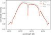 |
Fig. 5 Observed mean intensity (black) and derived fit (red) in the 617.3 nm spectral window. The inferred prefilter curve is plotted as a dashed gray line. The light-gray spectrum represents the FTS atlas multiplied by the prefilter curve. We obtained the fitted curve by multiplying the FTS spectrum by the prefilter curve and convolving the result with the nominal CRISP2 transmission profile. |
3.5 Datasets and model for LRE characterization
The profile of the LRE can be sampled by parking the HRE in a continuum wavelength close to the central wavelength of the prefilter and scanning in the spectral direction with the LRE:
![Mathematical equation: $\[I_{\mathrm{obs}}(\lambda)^{\mathrm{LRE}}=\frac{\int_{\lambda_0}^{\lambda_1}\left\{I_{\mathrm{FTS}}\left(\lambda^{\prime}\right) \cdot P\left(\lambda^{\prime}\right)\right\} \cdot \hat{T}_{\mathrm{CRISP} 2}\left(\lambda^{\prime}-\lambda, \lambda^{\prime}\right) \mathrm{d} \lambda^{\prime}}{\int_{\lambda_0}^{\lambda_1} \mathrm{~d} \lambda^{\prime}},\]$](/articles/aa/full_html/2026/07/aa58701-25/aa58701-25-eq24.png) (14)
(14)
where ![Mathematical equation: $\[\hat{T}_{\text {CRISP2}}\left(\lambda^{\prime}-\lambda, \lambda^{\prime}\right)\]$](/articles/aa/full_html/2026/07/aa58701-25/aa58701-25-eq25.png) is calculated with the HRE placed at a constant wavelength, while the LRE scans in the spectral direction (hence the double λ dependence in the notation). The LRE position can be regulated by adding an offset to the cavity error value. We cannot directly assume that the transmission profile is wavelength invariant. If we neglect the slow wavelength variation of the transmission profile and assume that the angular integral can be performed separately for each etalon, such that
is calculated with the HRE placed at a constant wavelength, while the LRE scans in the spectral direction (hence the double λ dependence in the notation). The LRE position can be regulated by adding an offset to the cavity error value. We cannot directly assume that the transmission profile is wavelength invariant. If we neglect the slow wavelength variation of the transmission profile and assume that the angular integral can be performed separately for each etalon, such that
![Mathematical equation: $\[\hat{T}_{\mathrm{HRE}}=\sum_{i=0}^{N_{\mathrm{ray}}-1} w_i \mathrm{e}^{-i k_4 \phi_4} T\left(R_H, C_H, \theta_i\right),\]$](/articles/aa/full_html/2026/07/aa58701-25/aa58701-25-eq26.png)
![Mathematical equation: $\[\hat{T}_{\mathrm{LRE}}=\sum_{i=0}^{N_{\mathrm{ray}}-1} w_i \mathrm{e}^{-i k_4 \phi_4} T\left(R_L, C_L, \theta_i\right),\]$](/articles/aa/full_html/2026/07/aa58701-25/aa58701-25-eq27.png) we can re-write the model as a convolution:
we can re-write the model as a convolution:
.\]$](/articles/aa/full_html/2026/07/aa58701-25/aa58701-25-eq28.png) (15)
(15)
We tested the validity of these two assumptions in Fig. A.1 (right panel). Our calculations show that the maximum difference between the predictions from Eqs. (14) and (15) is very small (±0.2% relative to the peak intensity) in the central part of the profile. Therefore, we consider this approximation adequate for the purposes of this study.
Given that the HRE profile is much narrower than the LRE profile, their convolution yields a train of LRE profiles centered at the locations of the HRE transmission peaks. The strength of the secondary peaks is modulated by the transmission of the prefilter. If the latter is not strictly symmetric and the HRE is not centered at the central wavelength of the prefilter, we expect asymmetries in the peak amplitude of secondary transmission lobes (see e.g., Fig. 6).
The weak transmission peaks at approximately ±1.7 Å originate from the first FSR peak of the LRE aligning with the second FSR peak of the HRE on the opposite side of the prefilter curve (see the lower panel in Fig. 6). This means that to model those peaks close to the center, our model must include at least the first FSR peaks of the LRE (at Δλ ≈ ±6.5 Å) and extend to two FSR peaks for the HRE. Since the determination of the prefilter in the far wings is less accurate than in the central part, and fitting one lobe should suffice to determine the cavity and reflectivity errors, we fit only the central peak, although the dataset and the model cover a much larger spectral range to properly reproduce the wings of the central lobe.
We derived the prefilter and HRE parameters, which also appear in Eq. (15), from the HRE fits for each pixel in the FOV and kept them constant for the LRE fits. However, we allowed the prefilter gain to change, as the LRE and HRE scans are not strictly simultaneous, and the intensity level may have changed. The model therefore has three free parameters per pixel (the gain factor, the LRE cavity separation, and the LRE reflectivity).
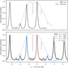 |
Fig. 6 Top: observed spatially averaged LRE (black) and HRE (dashed gray) spectral scans. Bottom: simulated LRE scans, including only the central lobes of the HRE and LRE (red), including the secondary HRE lobes at ±1 × FSR (blue), and including the secondary HRE peaks at ±2 × FSR and the LRE peaks at ±1 × FSR (black). The HRE profile is multiplied by an analytical estimate of the prefilter and the FTS atlas (shown in dashed gray). |
3.6 Code implementation
We implemented a Levenberg–Marquardt algorithm (Levenberg 1944; Marquardt 1963) to fit the data. The code is written in C++ with OpenMP parallelization. We created a Python interface for all routines1. We implemented the FPI functions using objectoriented programming, so that many quantities are only calculated once during class initialization and stored for subsequent calculations. All three transmission-profile approximations (see Sect. 3.1) and their analytical derivatives are available through the Python interface. We briefly describe the calculation of the analytical derivatives of the transmission profile and the prefilter curve in Appendices B and C. Our code uses the Eigen-3 linear algebra library (Guennebaud et al. 2010).
4 Results
We performed the calculations as follows:
We calculated initial estimates of the HRE and LRE cavity maps by fitting a parabola to the core of a spectral line (HRE) or to the intensity peak maximum (in the LRE dataset). We converted the wavelength shifts to cavity separation (Δλ/λ = −ΔC/C). The initial LRE cavity map was then compensated by using the HRE cavity map.
We fitted the HRE and prefilter parameters, while keeping the initial LRE cavity map constant.
Once the HRE and prefilter parameters were determined, we fitted the LRE parameters. The prefilter curve and HRE parameters were used to generate the LRE model.
We refined the HRE parameters from step 2 using the updated estimate of the LRE cavity map and reflectivities.
The LRE cavity map initialization in step 1 allows the HRE reflectivity to be determined without being affected by the assumption that the LRE is tuned at the reference wavelength or always co-tuned with the HRE. We recalculated the HRE parameters in step 4 using the final LRE cavity and reflectivity maps, initializing the fit from the results of step 1.
4.1 HRE parameter maps
We optimized the parameters of the model described in Eq. (13) for each pixel of the observed FOV, obtaining a 2D map for each of the model parameters. We first performed a fit on the mean spectrum over the entire FOV and used the resulting prefilter parameters as initial values for the 2D fits. An absolute wavelength calibration was obtained in this step, which we used to perform the translation from digital etalon offset units to a calibrated wavelength axis. This also allowed us to precisely determine where the LRE is parked in the LRE scan.
Figure 7 shows the spectra from three locations in the FOV and their corresponding best fits. We chose these points randomly, but at locations with remarkably different values of χ2, so that the reader can assess the quality of the fits in regions with low (red), medium (black) and large (blue) values of χ2. Even the example with the highest χ2 value represents an acceptable fit, as the spectral lines widths and shapes and the overall prefilter curve are reproduced by the model. Most discrepancies indicate small-scale structure (in the spectral direction) in the prefilter curve that cannot be fully captured by our model parametrization.
Fig. 8 shows the resulting model parameters. We do not show maps of pg because it has no scientific value in this study. The HRE cavity-error map (a) has a standard deviation of 2 nm (not to be confused with the RMS value of the wavelength shifts it induces in the spectrum). The HRE reflectivity map has a standard deviation of 0.46%. We measured both quantities over the entire circular FOV. They agree reasonably well with the instrument specifications, although the mean RHRE is 1.8% lower than the nominal factory value. This discrepancy could be explained by a small residual tilt angle in the HRE, which is compensated for in our model as a reduced reflectivity.
The 617.3 nm prefilter2 is slightly tilted to avoid reflections or interference patterns. This tilt shifts the center of the passband to shorter wavelengths and can affect the inferred FOV-dependent central-wavelength (e.g., Löfdahl et al. 2011). Additionally, there is a FOV variation of approximately ±1 Å (0.26 Å RMS). The prefilter FWHM also varies across the FOV, covering a range of approximately ±0.3 Å centered around 4.8 Å (0.04 Å RMS). The coefficients of the polynomial component capture the level of asymmetry (nonzero values in p0) and the deviations between the predicted shape given by 1/(1 + q2pncav) and the observations.
The reconstructed prefilter maps show spatial correlations between some parameters. They appear to mainly capture fringes, but their imprint in those parameters has a small amplitude. We also tried fixing some parameters to constant values, but the quality of the fits worsened. We allowed the model parameters to absorb the influence of fringes (present in the data) and obtained the best fit, so that the cavity error and reflectivity estimates are not affected by errors in the prefilter estimation.
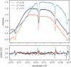 |
Fig. 7 Observed spectrum (dots) and best fit (solid line) from three locations in the FOV. We applied an offset of ±0.2 to the blue and red curves to improve readability. The locations of these points are indicated in panel (a) of Fig. 8 using the same color coding. The residues are normalized by the peak observed intensity of each curve. |
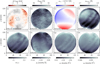 |
Fig. 8 Inferred parameter maps from the prefilter and HRE model. Panel (a) is the HRE cavity error map, (b) is the HRE reflectivity map, (c) is the prefilter central wavelength, (d) is the prefilter FWHM, and (e–g) are the coefficients of the polynomial prefilter components. The crosses indicated in (a) correspond to the fits shown in Fig. 7 using the same color coding. |
4.2 LRE parameter maps
The LRE model has only three parameters, but (as illustrated in Fig. 6) it generally requires knowledge of the spatially resolved prefilter curve and the HRE parameters that were derived in Sect. 4.1. These are passed as fixed inputs to the LRE fitting routines, while the gain factor of each pixel is fitted together with the LRE cavity error map and LRE reflectivity map. Accurate and consistent wavelength calibration of all datasets is required to properly fit the data, so that the prefilter curve derived with the HRE dataset is placed at the correct line positions of the LRE scan. The wavelength calibration performed with the FTS atlas using the mean spectrum allows an accurate translation from digital units to absolute wavelength, under the assumption that the etalon’s wavelength-offset calibration remains constant during the entire data-acquisition time. In our experience, this calibration is very stable over many hours or even days.
Fig. 9 shows the derived 2D maps and fit examples. We show fit examples that were chosen to represent a low χ2 (red), a pixel with a χ2 very close to the mean χ2 over the FOV (blue), and a large value of χ2 (black). Overall, the quality of the fits is very good. In early attempts that included the entire observed LRE spectral range, we noticed that most of the fit discrepancies originate from errors in the secondary transmission peaks (even the small peaks very close to the central peak), in the form of an amplitude error. These are modulated by the prefilter curve, which likely points to inaccuracies in the prefilter estimation in the very far wings. We note that the prefilter is derived from the HRE dataset, which in our case has a narrower wavelength coverage than the LRE scan, and therefore the prefilter in the outer points is not necessarily well constrained by the data but is instead assumed to follow the analytical description in Eq. (8).
We fit the central lobe in this part, which is very well reproduced by the model at all locations, even for larger χ2 values. The model itself includes the full range, but only the central lobe contributes to the computation of χ2. Including the full range is important to properly model the wings of the central lobe, since transmission peaks in the wings contribute significantly to the observed intensity. At 617.3 nm, the mean LRE reflectivity is RLRE = 88.66% and the RMS variation of the cavity errors is σCLRE = 2 nm.
4.3 Simplified models
We derive the parameter maps shown in Figs. 8 and 9 using the full calculation of the transmission profile. Furthermore, we include the secondary peaks located at ±1 × FSR in the calculation of the HRE model. Given the large size of the CRISP2 images (2560 × 2560 pixels2) and the large number of spectral points included in the model, this approach is computationally expensive.
We explored the effect of relaxing each of the model requirements to speed up the calculations. We first kept the full spectral range of the observations and performed the fits with approximated transmission profile recipes (perpendicular incidence, the conv approximation, and the full calculation). We then truncated the data (and the model) to include only the central lobe of the HRE and LRE in the fits, for all three transmission-profile recipes. Since this limited spectral range does not allow us to estimate the prefilter parameters, we used a much simpler model:
![Mathematical equation: $\[I_{\mathrm{obs}}(\lambda)=\left\{I_{\mathrm{FTS}}(\lambda) \cdot p_g\left(1.0+p_3 \Delta \lambda^{\prime}\right)\right\} * T_{\mathrm{CRISP} 2}(\lambda),\]$](/articles/aa/full_html/2026/07/aa58701-25/aa58701-25-eq29.png) (16)
(16)
where p3 describes the slope of the observed background continuum, Δλ′ = λ − λref, and λref is a reference wavelength, typically the central wavelength of the spectral range. The main difference appears in the inferred reflectivities of both etalons. In each case, we took the full-profile calculation over the full spectral range as a reference. Figure 10 shows 2D density plots of ![Mathematical equation: $\[R_{x}^{y}-R_{\text {ref}}^{\mathrm{E}}\]$](/articles/aa/full_html/2026/07/aa58701-25/aa58701-25-eq30.png) versus
versus ![Mathematical equation: $\[R_{\text {ref}}^{\mathrm{E}}\]$](/articles/aa/full_html/2026/07/aa58701-25/aa58701-25-eq31.png) (where x denotes the ray, conv, or full transmission-profile approximation, and y denotes whether we used the intensity-transmission-profile integral y = I or the complex electric-field transmission profile y = E) and for the cavity separation
(where x denotes the ray, conv, or full transmission-profile approximation, and y denotes whether we used the intensity-transmission-profile integral y = I or the complex electric-field transmission profile y = E) and for the cavity separation ![Mathematical equation: $\[C_{x}^{y}-C_{\text {ref}}^{\mathrm{E}}\]$](/articles/aa/full_html/2026/07/aa58701-25/aa58701-25-eq32.png) versus
versus ![Mathematical equation: $\[C_{\text {ref}}^{\mathrm{E}}\]$](/articles/aa/full_html/2026/07/aa58701-25/aa58701-25-eq33.png) . These results show the following effects:
. These results show the following effects:
A simpler transmission profile recipe yields a lower fitted reflectivity. By neglecting the profile broadening effect of the angular integral (in the perpendicular-incidence case), or by ignoring the LRE tilt angle in the conv approximation, the fitting routine can only compensate for the missing broadening by artificially reducing the inferred reflectivity.
Considering only the central transmission lobe of the profile, while neglecting the contribution of secondary peaks at ±1 × FSR, increases the spread in the inferred reflectivities. This effect is clearly visible when comparing the two columns of Fig. 10 for each transmission-profile recipe.
The mean value of the cavity error maps is on average very close to zero when the full spectral range is included. When only the central lobe is considered, the cavity errors have an offset of approximately 0.85 nm (corresponding to a shift of 67 mÅ).
The simplified transmission-profile recipe produces a larger spread around the mean, with a much greater spread for calculations that include the central lobe only (≤0.02–0.1 nm vs. ~0.2 nm).
A global offset in the derived parameters is manageable, whereas the spread is more problematic as it captures FOV-dependent errors that are harder (perhaps even impossible) to correct. For example, the conv approximation with the full spectral range shows a small spread in both quantities compared to the reference case, showing a slight offset in the inferred reflectivity that could be calibrated. The full calculation adopting an integral of the intensity transmission profile shows an even smaller spread and better captures the asymmetries in the real profile, but yields a larger reflectivity offset.
Fig. 11 shows similar results for the LRE, although in this case we only considered one spectral range. The LRE is broader and the cavity error determination appears to be less affected by the exact transmission profile recipe that is used in the calculation. The offset is approximately −0.11 nm and the spread is very small in all cases (≤0.009 nm). The reflectivity determination is more sensitive to simplifications that do not capture the tilt of the etalon. The conv calculation predicts a lower reflectivity than the single-ray approximation. However, after careful inspection of the fit quality (not shown), we conclude that the average value of χ2 is ~35% larger for the single-ray case, reflecting that this formula cannot capture the profile asymmetries induced by the angular integral and the tilt of the LRE.
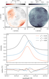 |
Fig. 9 Inferred parameter maps from the LRE model fit and three fit examples. Panel (a) is the LRE cavity error map, (b) is the LRE reflectivity map, and (c) illustrates three observed LRE scan spectra (dots) and the corresponding fits (solid line). The locations of these spectra in the FOV are marked by cross markers in panel a using the same color coding as in panel (c). We applied a vertical offset of ±0.35 to the red and black curves to improve readability. We normalized the residues by the peak observed intensity of each curve. |
4.4 Fast characterization of the instrumental profile
Figure 10 shows that simplified transmission-profile calculations can be compensated for by a biased adjustment of the inferred reflectivity. However, a separate question is how different the resulting CRISP2 profiles are for the various calculations. We computed the transmission profiles using the results of ![Mathematical equation: $\[R_{\text {full}}^{\mathrm{E}}\]$](/articles/aa/full_html/2026/07/aa58701-25/aa58701-25-eq34.png) ,
, ![Mathematical equation: $\[R_{\text {conv}}^{\mathrm{E}}\]$](/articles/aa/full_html/2026/07/aa58701-25/aa58701-25-eq35.png) , and
, and ![Mathematical equation: $\[R_{\text {full}}^{\mathrm{I}}\]$](/articles/aa/full_html/2026/07/aa58701-25/aa58701-25-eq36.png) and their corresponding formulas.
and their corresponding formulas.
The results (Fig. 13) show that if the goal of the fits is to characterize the instrumental profile (e.g., for inversions), the faster angular integration of the intensity profile may suffice. The residues in this figure are defined slightly different from those in the rest of the manuscript. Instead of dividing the difference by the peak intensity of each curve, they are normalized by the wavelength-dependent intensity. This makes differences between profiles easier to assess across the full wavelength range, although the errors appear large in regions of very low transmission. With this definition, the maximum relative error is approximately ~7% and generally within ±2%, although the peak error occurs in the secondary transmission lobes, where the transmission is very low compared to the central lobe. Both approximate formulas show a systematic offset in the far wings: the decay is slightly faster for ![Mathematical equation: $\[T_{\text {full}}^{I}\]$](/articles/aa/full_html/2026/07/aa58701-25/aa58701-25-eq37.png) and slower for
and slower for ![Mathematical equation: $\[T_{\text {conv}}^{E}\]$](/articles/aa/full_html/2026/07/aa58701-25/aa58701-25-eq38.png) . Using the complex angular integration while neglecting the LRE tilt yields larger deviations, with similar peak deviations but a larger mean deviation.
. Using the complex angular integration while neglecting the LRE tilt yields larger deviations, with similar peak deviations but a larger mean deviation.
These results suggest that the primary, though not only, source of profile broadening is the contribution from slanted rays in the angular integral, not phase errors, because relatively small adjustments in the inferred reflectivity can compensate for the latter. Faster inference algorithms or a faster forward calculation of the instrumental profile are useful when computational resources are limited.
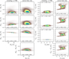 |
Fig. 10 2D histograms comparing the inferred HRE reflectivity and cavity errors to the reference case ( |
![Mathematical equation: $\[R_{x}^{y}-R_{\text {ref}}^{\mathrm{E}}\]$](/articles/aa/full_html/2026/07/aa58701-25/aa58701-25-eq39.png)
![Mathematical equation: $\[R_{\text {ref}}^{\mathrm{E}}\]$](/articles/aa/full_html/2026/07/aa58701-25/aa58701-25-eq40.png)
![Mathematical equation: $\[C_{x}^{y}-C_{\text {ref}}^{\mathrm{E}}\]$](/articles/aa/full_html/2026/07/aa58701-25/aa58701-25-eq41.png)
![Mathematical equation: $\[C_{\text {ref}}^{\mathrm{E}}\]$](/articles/aa/full_html/2026/07/aa58701-25/aa58701-25-eq42.png)
4.5 Flat-fielding and prefilter correction
The results of the HRE parametrization can be used to generate accurate flats that include the prefilter correction in a single step. In that case, the flat is given by Eq. (13) but without the Ifts factor. Gain tables must be generated for all wavelength tuning points simultaneously. Scharmer et al. (2013) used a similar approach. Figure 12 shows a 2D histogram of the HRE dataset divided by the flat-field correction. For this dataset, the expected result after the flat and prefilter correction is approximately Ifts · TCRISP2. The resulting spectrum shows very little spread in the continuum, which is very close to unity over the entire spectral range. In the lines, the spread is larger because data from a single wavelength bin can be distributed over a larger number of intensity bins in the vertical direction. The red curve shows the degraded FTS atlas profile, which is the reference used to evaluate whether the prefilter correction worked well over the entire wavelength range. With the exception of the bluest part at 6170 Å where the prefilter determination is less accurate, the overall agreement is very good.
The acquisition of flat-field data over such a large wavelength range is likely not feasible on a daily basis for all spectral lines that are commonly observed together with CRISP2. However, adding a few extra continuum points across the prefilter could suffice to estimate the prefilter parameters.
In comparison, the SST data reduction pipeline (SSTRED, de la Cruz Rodríguez et al. 2015; Löfdahl et al. 2021) estimates a template mean spectrum from the observed flat-field data (instead of using the FTS atlas) and models the FOV-dependent spectra by applying a shift that mimics cavity errors and multiplying by a polynomial that captures FOV-dependent variations of the prefilter. A global prefilter curve is estimated in a separate step and applied to the reduced data after image reconstruction. This approach is robust because it does not assume anything about the observed spectrum (i.e., it does not need to be similar to the FTS atlas) and it is insensitive to the exact imprint of tellurics in the FTS spectrum, which differ from those in the observations.
In the near future, we plan to implement the model from Sect. 4.3 in SSTRED.
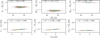 |
Fig. 11 2D histograms comparing the inferred LRE reflectivity and cavity error maps to the reference case. The reference case is the “full” complex calculation. The upper row shows the reflectivity results and the bottom row shows the cavity errors. The label “E” indicates that the angular integral was performed over the electric field transmission profile, whereas the “I” super-index corresponds to a direct integral of the per-ray intensity transmission profile. |
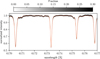 |
Fig. 12 Prefilter-corrected 2D histogram of the observed data. Each wavelength bin is normalized by the total to better illustrate the spread of the data points. The cavity error map is compensated in the wavelength array at each (x, y) location in the FOV. The red curve shows the FTS atlas multiplied by the prefilter, convolved with the CRISP2 transmission profile, and divided again by the prefilter curve, also convolved with the CRISP2 transmission profile. |
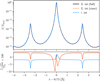 |
Fig. 13 Transmission profiles of the CRISP2 instrument calculated from the inferred reflectivities at the center of the FOV (x, y) = (nx/2, ny/2). Top panel: peak-normalized transmission profiles corresponding to the “full” complex calculation (black), the “conv” complex calculation (red), and the “full” integration of the intensity vector (blue). Bottom panel: residues relative to the “full” complex calculation. We normalized the residues by the observed intensity of each curve per wavelength. |
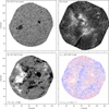 |
Fig. 14 Dataset from CRISP2 acquired in the FeI 617.3 nm and Hα lines on October 10, 2025 at 09:50:40 UT. Bottom panels: results of a Milne-Eddington inversion using the 617.3 nm dataset. Top left: continuum image at 617.4 nm. Top right: Hα core image. Bottom left: line-of-sight component of the magnetic field vector, clipped at ±70 G. Bottom right: cavity-error-map-compensated line-of-sight velocity, clipped at ±4 km s−1. Data courtesy of A. Brunvoll, R. Nguyen, and L. Rouppe van der Voort (University of Oslo). |
4.6 Example dataset
Figure 14 shows two quasi-monochromatic images acquired with CRISP2 in the 617.3 nm continuum and the core of the Hα line. Additionally, we performed a spatially and temporally regularized Milne-Eddington inversion (de la Cruz Rodríguez 2019; de la Cruz Rodríguez & Leenaarts 2024) of the FeI 617.3 nm dataset. We display the derived line-of-sight components of the magnetic and velocity fields, corrected for cavity errors. We processed the data with the SSTRED pipeline (Löfdahl et al. 2021; de la Cruz Rodríguez et al. 2015) and the multi-object-multi-frame blind deconvolution image reconstruction technique (MOMFBD; van Noort et al. 2005; Löfdahl 2002). These data and inversion results show no systematic errors or artifacts indicative of poor instrumental performance.
Although these data provide an unprecedentedly large FOV for this type of instrument and spatial resolution, the current FOV is limited by the modulator size and the 617.3 nm prefilter. Both will be replaced during 2026 with larger versions that will enable the use of the full physically available FOV.
5 Conclusions
We propose a method, together with several simplifications, that enables full characterization of dual-etalon FPI systems, including the parameters of order-selecting prefilters, from observational data. This method can therefore be applied at any wavelength for which an order-selecting prefilter is available, without changing the optical setup. Compared with laser-based measurements, where the laser is placed on the optical table, our approach has the advantage of including the broadening effect of the slowly-converging telecentric beam, which such laser measurements cannot capture.
We performed a full characterization of the new CRISP2 dual-etalon FPI parameters at 617.3 nm. The FOV-dependent cavity separation errors are small, with RMS values ~2.0 nm for both etalons. The etalon reflectivities show RMS variations of 0.45 and 0.33% for the HRE and LRE, respectively, at 617.3 nm. At other wavelengths, the overall field dependence should behave similarly, although the average reflectivity will obviously change.
We assessed the effect of using simplified transmission-profile approximations and reduced spectral coverage when inferring the FPI parameters. Simplified transmission-profile approximations systematically yield lower inferred reflectivities, whereas reduced spectral coverage also introduces a large dispersion in the inferred reflectivities. Our results suggest that the conv approximation can be used to determine HRE reflectivities at a minimal accuracy cost. We therefore recommend using at least the conv approximation for HRE parameter determination, since it requires only a small set of incident angles and yields similar results to the full calculation. For the LRE, the model has fewer parameters and the restricted spectral range allows for fast estimation using the full approach.
If the sole goal is to characterize the FOV-dependent transmission profile of the system, without further interpretation of the derived etalon reflectivities, our results suggest that the faster (approximated) angular integration of the intensity transmission profile yields very similar results to the full complex integration of the electric field transmission profile. In this case, the reflectivity is modified to compensate for inaccuracies in the profile calculation, while the resulting transmission profiles remain virtually identical in shape and area, although not in peak transmission.
We show that estimating the prefilter curve across the FOV is generally required to characterize the HRE and LRE reflectivities. However, if the prefilter is sufficiently narrow compared to the FSR of the FPI, the secondary transmission lobes will be damped when observing at the center of the prefilter. Our results suggest that such cases can be reasonably well modeled without including transmission peaks at ±1×FSR. In such cases, regular flat-field data may suffice.
Modern inversion codes allow the use of FOV-dependent spectral transmission profiles, including NICOLE (Socas-Navarro et al. 2015), SNAPI (Milić & van Noort 2018), STiC (de la Cruz Rodríguez et al. 2019), and FIRTEZ-dz (Pastor Yabar et al. 2019). This feature is very important because of the FOV-dependent variations of the spectral transmission profile (wavelength shift and broadening variations) that are imprinted in FPI observations.
All codes used in this study are publicly available3 together with documented examples. We hope that they will be useful to the solar community in the characterization of future telecentric FPI instruments at the Daniel K. Inouye Solar Telescope (Rimmele et al. 2020) and the European Solar Telescope (Quintero Noda et al. 2022).
Acknowledgements
We are very thankful to the anonymous referee of this paper, for providing very constructive comments and suggestions that clearly improved the quality of the study. The Institute for Solar Physics is supported by a grant for research infrastructures of national importance from the Swedish Research Council (registration number 2021-00169). The Swedish 1-m Solar Telescope is operated on the island of La Palma by the Institute for Solar Physics of Stockholm University in the Spanish Observatorio del Roque de los Muchachos of the Instituto de Astrofísica de Canarias. This project has been funded by the European Union through the European Research Council (ERC) under the Horizon Europe program (MAGHEAT, grant agreement 101088184). The European Solar Telescope project is supported by a grant for research infrastructures from the Swedish Research Council (registration number 2023-00169). Code debugging was possible thanks to resources provided by the National Academic Infrastructure for Supercomputing in Sweden (project NAISS 2025-1-9) at the PDC Centre for High Performance Computing (PDC-HPC) at the Royal Institute of Technology in Stockholm. We are very grateful to L. Rouppe van der Voort for providing the dataset shown in Fig. 14.
References
- Bailén, F. J., Orozco Surárez, D., & del Toro Iniesta, J. C. 2019a, ApJS, 241, 9 [CrossRef] [Google Scholar]
- Bailén, F. J., Orozco Suárez, D., & del Toro Iniesta, J. C. 2019b, ApJS, 242, 21 [Google Scholar]
- Bailén, F. J., Orozco Suárez, D., & del Toro Iniesta, J. C. 2020, ApJS, 246, 17 [Google Scholar]
- Bailén, F. J., Orozco Suárez, D., & del Toro Iniesta, J. C. 2021, ApJS, 254, 18 [CrossRef] [Google Scholar]
- Born, M., & Wolf, E. 2019, Principles of Optics: 60th Anniversary Edition, 7th edn. (Cambridge: Cambridge University Press) [Google Scholar]
- Cavallini, F. 2006, Sol. Phys., 236, 415 [NASA ADS] [CrossRef] [Google Scholar]
- de la Cruz Rodríguez, J. 2010, Instrumental characterization of SST/CRISP from observations, https://dubshen.astro.su.se/~jaime/delacruz_nproj_2010.pdf, report of a self-study PhD course, Dept. of Astronomy, Stockholm University [Google Scholar]
- de la Cruz Rodríguez, J. 2019, A&A, 631, A153 [NASA ADS] [CrossRef] [EDP Sciences] [Google Scholar]
- de la Cruz Rodríguez, J., Löfdahl, M. G., Sütterlin, P., Hillberg, T., & Rouppe van der Voort, L. 2015, A&A, 573, A40 [NASA ADS] [CrossRef] [EDP Sciences] [Google Scholar]
- de la Cruz Rodríguez, J., Leenaarts, J., Danilovic, S., & Uitenbroek, H. 2019, A&A, 623, A74 [Google Scholar]
- de la Cruz Rodríguez, J., & Leenaarts, J. 2024, A&A, 685, A85 [NASA ADS] [CrossRef] [EDP Sciences] [Google Scholar]
- del Toro Iniesta, J. C., Orozco Suárez, D., Álvarez-Herrero, A., et al. 2025, Sol. Phys., 300, 148 [Google Scholar]
- del Toro Iniesta, J. C., & Ruiz Cobo, B. 2016, Liv. Rev. Sol. Phys., 13, 4 [Google Scholar]
- Dravins, D., Lindegren, L., & Nordlund, A. 1981, A&A, 96, 345 [NASA ADS] [Google Scholar]
- Felipe, T., Socas-Navarro, H., & Przybylski, D. 2018, A&A, 614, A73 [NASA ADS] [CrossRef] [EDP Sciences] [Google Scholar]
- Guennebaud, G., Jacob, B., et al. 2010, Eigen v3, http://eigen.tuxfamily.org [Google Scholar]
- Hecht, E. 2017, Optics (Oxford: Pearson Education, Incorporated) [Google Scholar]
- Levenberg, K. 1944, Quarterly Appl. Math., 2, 164 [Google Scholar]
- Löfdahl, M. G. 2002, SPIE Conf. Ser., 4792, 146 [Google Scholar]
- Löfdahl, M. G., Henriques, V. M. J., & Kiselman, D. 2011, A&A, 533, A82 [NASA ADS] [CrossRef] [EDP Sciences] [Google Scholar]
- Löfdahl, M. G., Hillberg, T., de la Cruz Rodríguez, J., et al. 2021, A&A, 653, A68 [Google Scholar]
- Marquardt, D. W. 1963, J. Soc. Industrial Appl. Math., 11, 431 [Google Scholar]
- Milić, I., & van Noort, M. 2018, A&A, 617, A24 [Google Scholar]
- Neckel, H., & Labs, D. 1984, Sol. Phys., 90, 205 [Google Scholar]
- Pastor Yabar, A., Borrero, J. M., & Ruiz Cobo, B. 2019, A&A, 629, A24 [NASA ADS] [CrossRef] [EDP Sciences] [Google Scholar]
- Quintero Noda, C., Schlichenmaier, R., Bellot Rubio, L. R., et al. 2022, A&A, 666, A21 [NASA ADS] [CrossRef] [EDP Sciences] [Google Scholar]
- Reardon, K. P., & Cavallini, F. 2008, A&A, 481, 897 [NASA ADS] [CrossRef] [EDP Sciences] [Google Scholar]
- Rimmele, T. R., Warner, M., Keil, S. L., et al. 2020, Sol. Phys., 295, 172 [Google Scholar]
- Rouppe van der Voort, L. H. M., van Noort, M., & de la Cruz Rodríguez, J. 2023, A&A, 673, A11 [NASA ADS] [CrossRef] [EDP Sciences] [Google Scholar]
- Santamarina Guerrero, P., Orozco Suárez, D., Bailén, F. J., & Blanco Rodríguez, J. 2024, A&A, 688, A67 [NASA ADS] [CrossRef] [EDP Sciences] [Google Scholar]
- Scharmer, G. B. 2006, A&A, 447, 1111 [NASA ADS] [CrossRef] [EDP Sciences] [Google Scholar]
- Scharmer, G. B., Bjelksjo, K., Korhonen, T. K., Lindberg, B., & Petterson, B. 2003, SPIE Conf. Ser., 4853, 341 [NASA ADS] [Google Scholar]
- Scharmer, G. B., de la Cruz Rodriguez, J., Sütterlin, P., & Henriques, V. M. J. 2013, A&A, 553, A63 [NASA ADS] [CrossRef] [EDP Sciences] [Google Scholar]
- Scharmer, G. B., de la Cruz Rodríguez, J., Leenaarts, J., et al. 2026, A&A, 705, A55 [NASA ADS] [CrossRef] [EDP Sciences] [Google Scholar]
- Schlichenmaier, R., Pitters, D., Borrero, J. M., & Schubert, M. 2023, A&A, 669, A78 [NASA ADS] [CrossRef] [EDP Sciences] [Google Scholar]
- Schnerr, R. S., de La Cruz Rodríguez, J., & van Noort, M. 2011, A&A, 534, A45 [NASA ADS] [CrossRef] [EDP Sciences] [Google Scholar]
- Schubert, M., Kentischer, T., & von der Lühe, O. 2017, J. Astron. Telesc. Instrum. Syst., 3, 045002 [Google Scholar]
- Socas-Navarro, H., de la Cruz Rodríguez, J., Asensio Ramos, A., Trujillo Bueno, J., & Ruiz Cobo, B. 2015, A&A, 577, A7 [NASA ADS] [CrossRef] [EDP Sciences] [Google Scholar]
- Solanki, S. K., del Toro Iniesta, J. C., Woch, J., et al. 2020, A&A, 642, A11 [NASA ADS] [CrossRef] [EDP Sciences] [Google Scholar]
- van Noort, M., Rouppe van der Voort, L., & Löfdahl, M. G. 2005, Sol. Phys., 228, 191 [Google Scholar]
- van Noort, M. J., & Rouppe van der Voort, L. H. M. 2006, ApJ, 648, L67 [NASA ADS] [CrossRef] [Google Scholar]
- von der Lühe, O., & Kentischer, T. J. 2000, A&AS, 146, 499 [Google Scholar]
These codes, along with documented examples, are publicly available on https://github.com/jaimedelacruz/pyFPI
This prefilter was manufactured by Alluxa.
Appendix A Assumption of a constant transmission profile in the models
The transmission profile of an etalon is wavelength dependent. This dependency is contained in the phase term and in the wavelength variation of the etalon reflectivity. To speed-up calculations, we have assumed that the CRISP2 transmission profile can be assumed to be constant within the wavelength range covered by the prefilter. We have assessed the validity of this assumption in both HRE and LRE models. Figure A.1 illustrates the results of performing the convolutions in both models with a constant transmission profile as a function of wavelength (black curve) and a wavelength-dependent transmission profile (red curve).
Within the range of the prefilter in the HRE model, errors are < ±1%. The approximations adopted in the LRE model yield a prediction with a maximum discrepancy of ±0.2% in comparison with that including a wavelength-varying instrumental profile. We argue that the assumption of a wavelength-invariant transmission profile within the wavelength ranges considered in our study is a good approximation that allows for a much quicker processing of very large FOVs.
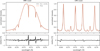 |
Fig. A.1 Simulated data assuming a constant transmission profile calculation (black curve, calculated at λ = 6173 Å) and a wavelength varying transmission profile (red curve). The latter was recalculated for each wavelength point with updated reflectivity and wavelength values. Left: Simulated HRE dataset using the FTS atlas and a symmetric prefilter curve centered at 6173 Å and a FWHM of 4.8. Right: Simulated LRE dataset using the same prefilter parameters as in the HRE calculation. The residues are normalized by the peak observed intensity of each curve. |
Appendix B Analytical derivatives of the FPI transmission profile
For any given incidence angle θ, the derivative of the transmission profile of an etalon relative to the cavity separation and reflectivity (see Eq. 1) can be trivially estimated:
![Mathematical equation: $\[\frac{\partial T(C, R, \lambda)}{\partial R}=\frac{T}{1-R}+\frac{1}{1-R}\left[\frac{-\cos (\psi / 2)+i ~\sin (\psi / 2)}{1+F ~\sin ^2(\psi / 2)}-T \frac{\sin ^2(\psi / 2)}{1+F ~\sin ^2(\psi / 2)} \frac{4(1+R)}{(1-R)^3}\right],\]$](/articles/aa/full_html/2026/07/aa58701-25/aa58701-25-eq43.png) (B.1)
(B.1)
![Mathematical equation: $\[\frac{\partial T(C, R, \lambda)}{\partial C}=\left[\frac{1}{1-R} \frac{(R-1) ~\sin (\psi / 2)+i(1+R) ~\cos (\psi / 2)}{1+F ~\sin ^2(\psi / 2)}-T \frac{2 F ~\sin (\psi / 2) ~\cos (\psi / 2)}{1+F ~\sin ^2(\psi / 2)}\right] \frac{2 \pi n ~\cos (\theta)}{\lambda},\]$](/articles/aa/full_html/2026/07/aa58701-25/aa58701-25-eq44.png) (B.2)
(B.2)
where T is the transmission profile (also in the right-hand-side).
We note though that the resulting FPI profile is not area normalized. The sin(ψ/2) and cos (ψ/2) terms in Eq. 1 generate an infinite succession of transmission peaks that has no general analytical integral. But assuming that we are operating on a regular (discrete) wavelength grid within a finite wavelength domain, the area of that transmission profile can be estimated as Atr = ∑iT(C, R, λi) (dropping the δλ factor as it vanishes in the convolution). The normalized (discrete) profile is given by:
![Mathematical equation: $\[T_n=\frac{T(C, R)}{A_{t r}}.\]$](/articles/aa/full_html/2026/07/aa58701-25/aa58701-25-eq45.png) (B.3)
(B.3)
The only thing we need to know is the derivative of the profile area relative to the cavity separation and the etalon reflectivity. For very small perturbations, changing the cavity separations only produces a displacement of the transmission profile and the area remains the same. The reflectivity derivative is already given in Eq. B.1 and it is wavelength dependent. By defining Btr = ∑i ∂T(C, R, λi)/∂R, we can easily calculate the derivative of the area normalized profile using the chain rule as:
![Mathematical equation: $\[\frac{\partial T_n(C, R)}{\partial R}=\frac{1}{A_{t r}}\left(\frac{\partial T(C, R)}{\partial R}-\frac{B_{t r}}{A_{t r}} T(C, R)\right).\]$](/articles/aa/full_html/2026/07/aa58701-25/aa58701-25-eq46.png) (B.4)
(B.4)
Figure B.1 depicts a comparison between analytical and numerical derivatives of the area-normalized transmission profile at 630.2 nm using the nominal reflectivities and cavity separations of the etalons.
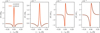 |
Fig. B.1 Derivatives of the area-normalized transmission profile relative to the reflectivity (R) and cavity separation (C) of each of the etalons. The analytical calculation is depicted in red and the numerical ones are indicated with black dots. |
Appendix C Analytical derivatives of the prefilter transmission profile
The derivatives of the prefilter parameters can be easily derived in analytical form, which we include here for completeness. For a given λ and Δλ = λ − pw0:
![Mathematical equation: $\[\frac{\partial P}{\partial p_g}=\frac{1}{1+q^{2 p_{\mathrm{ncav}}}}\left(1+w_{\mathrm{apod}}\left(p_0 \Delta \lambda+p_1 \Delta \lambda^2+p_2 \Delta \lambda^3\right)\right),\]$](/articles/aa/full_html/2026/07/aa58701-25/aa58701-25-eq47.png) (C.1)
(C.1)
![Mathematical equation: $\[\frac{\partial P}{\partial p_{w_0}}=2 \frac{p_g}{\left(1+q^{2 p_{\text {ncav }}}\right)^2} \frac{q^{2 p_{\text {ncav }}-1} \cdot \operatorname{sign}(q)}{p_{\text {fwhm }}}\left(1+w_{\text {apod }}\left(p_0 \Delta \lambda+p_1 \Delta \lambda^2+p_2 \Delta \lambda^3\right)\right)-\frac{p_g w_{\text {apod }}}{1+q^{2 p_{\text {ncav }}}}\left(p_0+2 p_1 \Delta \lambda+3 p_2 \Delta \lambda^2\right),\]$](/articles/aa/full_html/2026/07/aa58701-25/aa58701-25-eq48.png) (C.2)
(C.2)
![Mathematical equation: $\[\frac{\partial P}{\partial p_{\text {fwhm }}}=\frac{p_g}{\left(1+q^{2 p_{\text {ncav }}}\right)^2} \frac{q^{2 p_{\text {ncav }}-1} \cdot|q|}{p_{\text {fwhm }}}\left(1+w_{\text {apod }}\left(p_0 \Delta \lambda+p_1 \Delta \lambda^2+p_2 \Delta \lambda^3\right)\right),\]$](/articles/aa/full_html/2026/07/aa58701-25/aa58701-25-eq49.png) (C.3)
(C.3)
![Mathematical equation: $\[\frac{\partial P}{\partial p_0}=\frac{p_g}{1+q^{2 p_{\text {ncav }}}} w_{\text {apod}} \Delta \lambda,\]$](/articles/aa/full_html/2026/07/aa58701-25/aa58701-25-eq50.png) (C.4)
(C.4)
![Mathematical equation: $\[\frac{\partial P}{\partial p_1}=\frac{\partial P}{\partial p_0} w_{\text {apod}} \Delta \lambda,\]$](/articles/aa/full_html/2026/07/aa58701-25/aa58701-25-eq51.png) (C.5)
(C.5)
![Mathematical equation: $\[\frac{\partial P}{\partial p_2}=\frac{\partial P}{\partial p_1} w_{\text {apod}} \Delta \lambda,\]$](/articles/aa/full_html/2026/07/aa58701-25/aa58701-25-eq52.png) (C.6)
(C.6)
where q = 2(λ − pw0)/pfwhm, and Δλ = λ − pw0. Fig. C.1 illustrates the derivatives of the prefilter curve relative to all parameters.
Our definition of the apodization window is analytical, differentiable and it has a dependence on pw0 and pfwhm. For a given Δλ = λ − pw0, the derivatives of the apodization window are:
![Mathematical equation: $\[\frac{\partial w_{\mathrm{apod}}}{\partial p_{w_0}}=-\frac{\pi}{2 a_{\mathrm{scl}} p_{\mathrm{fwhm}}}\left(\left(1-\tanh ^2\left(\Delta \lambda_1\right)\right) \cdot\left(1-\tanh \left(\Delta \lambda_2\right)\right)+\left(1+\tanh \left(\Delta \lambda_1\right)\right) \cdot\left(\tanh ^2\left(\Delta \lambda_2\right)-1\right)\right),\]$](/articles/aa/full_html/2026/07/aa58701-25/aa58701-25-eq54.png) (C.8)
(C.8)
![Mathematical equation: $\[\frac{\partial w_{\mathrm{apod}}}{\partial p_{\mathrm{fwhm}}}=-\frac{\pi}{2 a_{\mathrm{scl}}} \frac{(\Delta \lambda) \cdot \operatorname{sign}(\Delta \lambda)}{p_{\mathrm{fwhm}}^2}\left(\left(1-\tanh ^2\left(\Delta \lambda_1\right)\right) \cdot\left(1-\tanh \left(\Delta \lambda_2\right)\right)-\left(1+\tanh \left(\Delta \lambda_1\right)\right) \cdot\left(\tanh ^2\left(\Delta \lambda_2\right)-1\right)\right).\]$](/articles/aa/full_html/2026/07/aa58701-25/aa58701-25-eq55.png) (C.9)
(C.9)
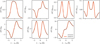 |
Fig. C.1 Derivatives of the prefilter curve with respect to all seven parameters considered in Eq. 8. The red curve illustrates the analytical derivatives and the black dots the finite-differences ones. These derivatives include the effect of the apodization window. |
Therefore, this dependence must be propagated to the derivatives of the prefilter curve relative to pw0 and pfwhm by adding the corresponding terms:
![Mathematical equation: $\[\left.\frac{\partial P}{\partial p_{w_0}}\right|_{\text {full }}=\frac{\partial P}{\partial p_{w_0}}+\frac{p_g}{1+q^{2 p_{\text {ncav }}}} \cdot\left(p_0 \Delta \lambda+p_1 \Delta \lambda^2+p_2 \Delta \lambda^3\right) \frac{\partial w_{\text {apod }}}{\partial p_{w_0}},\]$](/articles/aa/full_html/2026/07/aa58701-25/aa58701-25-eq56.png) (C.10)
(C.10)
![Mathematical equation: $\[\left.\frac{\partial P}{\partial p_{\mathrm{fwhm}}}\right|_{\mathrm{full}}=\frac{\partial P}{\partial p_{\mathrm{fwhm}}}+\frac{p_g}{1+q^{2 p_{\mathrm{ncav}}}} \cdot\left(p_0 \Delta \lambda+p_1 \Delta \lambda^2+p_2 \Delta \lambda^3\right) \frac{\partial w_{\mathrm{apod}}}{\partial p_{\mathrm{fwhm}}}.\]$](/articles/aa/full_html/2026/07/aa58701-25/aa58701-25-eq57.png) (C.11)
(C.11)
All Tables
All Figures
|
Fig. 1 Transmission profile at 617.3 nm measured with CRISP2. Top: high-resolution etalon (HRE), low-resolution etalon (LRE) and full transmission profiles, with the prefilter shape also indicated. Bottom: transmission profile and the same profile multiplied by the prefilter transmission, illustrating the attenuation of secondary lobes by the prefilter. |
| In the text | |
|
Fig. 2 Factory-measured reflectivities of the etalons (red) and the corresponding instrumental profile full width at half maximum (FWHM) for the CRISP2 instrument (black). The solid red line depicts the reflectivity of the high-resolution etalon, whereas the dashed red line corresponds to the reflectivity of the low-resolution etalon. We calculated the FWHM of the profile assuming perfect co-tuning of the profiles from the two etalons and the factory nominal reflectivities. |
| In the text | |
|
Fig. 3 Distribution of inclination angles across the (circular) pupil for a non-tilted case (α = 0, top left) and a tilt of α = 1/2F in the y axis (top right). Bottom panels: 2D histograms correlating the angles of the two cases (left: Nrays = 19, right: Nrays = 7). The histograms provide the integration weights used to perform the angular integral of the transmission profile over the pupil angles. |
| In the text | |
|
Fig. 4 Transmission profiles of the CRISP2 instrument calculated including instrument refocus (black), no refocus (blue), and by performing the angular integral directly on the intensity transmission profiles (dashed red). The profiles in the right panel are peak normalized. |
| In the text | |
|
Fig. 5 Observed mean intensity (black) and derived fit (red) in the 617.3 nm spectral window. The inferred prefilter curve is plotted as a dashed gray line. The light-gray spectrum represents the FTS atlas multiplied by the prefilter curve. We obtained the fitted curve by multiplying the FTS spectrum by the prefilter curve and convolving the result with the nominal CRISP2 transmission profile. |
| In the text | |
|
Fig. 6 Top: observed spatially averaged LRE (black) and HRE (dashed gray) spectral scans. Bottom: simulated LRE scans, including only the central lobes of the HRE and LRE (red), including the secondary HRE lobes at ±1 × FSR (blue), and including the secondary HRE peaks at ±2 × FSR and the LRE peaks at ±1 × FSR (black). The HRE profile is multiplied by an analytical estimate of the prefilter and the FTS atlas (shown in dashed gray). |
| In the text | |
|
Fig. 7 Observed spectrum (dots) and best fit (solid line) from three locations in the FOV. We applied an offset of ±0.2 to the blue and red curves to improve readability. The locations of these points are indicated in panel (a) of Fig. 8 using the same color coding. The residues are normalized by the peak observed intensity of each curve. |
| In the text | |
|
Fig. 8 Inferred parameter maps from the prefilter and HRE model. Panel (a) is the HRE cavity error map, (b) is the HRE reflectivity map, (c) is the prefilter central wavelength, (d) is the prefilter FWHM, and (e–g) are the coefficients of the polynomial prefilter components. The crosses indicated in (a) correspond to the fits shown in Fig. 7 using the same color coding. |
| In the text | |
|
Fig. 9 Inferred parameter maps from the LRE model fit and three fit examples. Panel (a) is the LRE cavity error map, (b) is the LRE reflectivity map, and (c) illustrates three observed LRE scan spectra (dots) and the corresponding fits (solid line). The locations of these spectra in the FOV are marked by cross markers in panel a using the same color coding as in panel (c). We applied a vertical offset of ±0.35 to the red and black curves to improve readability. We normalized the residues by the peak observed intensity of each curve. |
| In the text | |
|
Fig. 10 2D histograms comparing the inferred HRE reflectivity and cavity errors to the reference case ( |
| In the text | |
|
Fig. 11 2D histograms comparing the inferred LRE reflectivity and cavity error maps to the reference case. The reference case is the “full” complex calculation. The upper row shows the reflectivity results and the bottom row shows the cavity errors. The label “E” indicates that the angular integral was performed over the electric field transmission profile, whereas the “I” super-index corresponds to a direct integral of the per-ray intensity transmission profile. |
| In the text | |
|
Fig. 12 Prefilter-corrected 2D histogram of the observed data. Each wavelength bin is normalized by the total to better illustrate the spread of the data points. The cavity error map is compensated in the wavelength array at each (x, y) location in the FOV. The red curve shows the FTS atlas multiplied by the prefilter, convolved with the CRISP2 transmission profile, and divided again by the prefilter curve, also convolved with the CRISP2 transmission profile. |
| In the text | |
|
Fig. 13 Transmission profiles of the CRISP2 instrument calculated from the inferred reflectivities at the center of the FOV (x, y) = (nx/2, ny/2). Top panel: peak-normalized transmission profiles corresponding to the “full” complex calculation (black), the “conv” complex calculation (red), and the “full” integration of the intensity vector (blue). Bottom panel: residues relative to the “full” complex calculation. We normalized the residues by the observed intensity of each curve per wavelength. |
| In the text | |
|
Fig. 14 Dataset from CRISP2 acquired in the FeI 617.3 nm and Hα lines on October 10, 2025 at 09:50:40 UT. Bottom panels: results of a Milne-Eddington inversion using the 617.3 nm dataset. Top left: continuum image at 617.4 nm. Top right: Hα core image. Bottom left: line-of-sight component of the magnetic field vector, clipped at ±70 G. Bottom right: cavity-error-map-compensated line-of-sight velocity, clipped at ±4 km s−1. Data courtesy of A. Brunvoll, R. Nguyen, and L. Rouppe van der Voort (University of Oslo). |
| In the text | |
|
Fig. A.1 Simulated data assuming a constant transmission profile calculation (black curve, calculated at λ = 6173 Å) and a wavelength varying transmission profile (red curve). The latter was recalculated for each wavelength point with updated reflectivity and wavelength values. Left: Simulated HRE dataset using the FTS atlas and a symmetric prefilter curve centered at 6173 Å and a FWHM of 4.8. Right: Simulated LRE dataset using the same prefilter parameters as in the HRE calculation. The residues are normalized by the peak observed intensity of each curve. |
| In the text | |
|
Fig. B.1 Derivatives of the area-normalized transmission profile relative to the reflectivity (R) and cavity separation (C) of each of the etalons. The analytical calculation is depicted in red and the numerical ones are indicated with black dots. |
| In the text | |
|
Fig. C.1 Derivatives of the prefilter curve with respect to all seven parameters considered in Eq. 8. The red curve illustrates the analytical derivatives and the black dots the finite-differences ones. These derivatives include the effect of the apodization window. |
| In the text | |
Current usage metrics show cumulative count of Article Views (full-text article views including HTML views, PDF and ePub downloads, according to the available data) and Abstracts Views on Vision4Press platform.
Data correspond to usage on the plateform after 2015. The current usage metrics is available 48-96 hours after online publication and is updated daily on week days.
Initial download of the metrics may take a while.