


| Issue |
A&A
Volume 710, June 2026
|
|
|---|---|---|
| Article Number | L35 | |
| Number of page(s) | 6 | |
| Section | Letters to the Editor | |
| DOI | https://doi.org/10.1051/0004-6361/202659932 | |
| Published online | 24 June 2026 | |
Letter to the Editor
Shape and spin axis determination of the Tianwen-2 target asteroid (469219) Kamo’oalewa from light-curve inversion
1
BSA Osservatorio (K76), Strada Collarelle 53, 12038 Savigliano, Cuneo, Italy
2
Charles University, Faculty of Mathematics and Physics, Institute of Astronomy, V Holešovičkách 2, 18000 Prague, Czech Republic
3
Laboratoire Lagrange, Centre National de la Recherche Scientifique, Observatoire de la Côte d’Azur, Université Côte d’Azur, 06304 Nice, France
4
University of Leicester, School of Physics and Astronomy, University Road, LE1 7RH, Leicester, UK
★ Corresponding author: This email address is being protected from spambots. You need JavaScript enabled to view it.
Received:
18
March
2026
Accepted:
29
April
2026
Abstract
Context. Near-Earth asteroid (469219) Kamo’oalewa is an Earth quasi-satellite, temporarily trapped in a 1:1 orbital resonance with our planet. Despite its dynamical relevance and the hypothesis that it may be a lunar ejecta fragment, its physical properties are still poorly constrained. In particular, no reliable models of its shape and spin state have been published so far. The scientific interest in this object is further enhanced by its selection as the primary target of the Chinese Tianwen-2 mission, which aims to meet with this asteroid and return samples of it to Earth.
Aims. The aim of this work is to determine the shape and spin axis orientation of Kamo’oalewa by means of photometric telescope observations and light-curve inversion.
Methods. We analysed light curves obtained during several apparitions using the well-established algorithm, based on convex shape modelling.
Results. We derived a convex shape model and estimated the spin pole orientation. In the preferred solution, the pole is located at ecliptic coordinates λ, β = (126, −16)°, with a sidereal rotation period of P = 0.465 h.
Conclusions. Our results provide the first direct constraints on the rotational state and morphology of Kamo’oalewa, which is information of key importance in preparation for the upcoming Tianwen-2 sample-return mission.
Key words: minor planets / asteroids: general / minor planets / asteroids: individual: (469219) Kamo’oalewa
© The Authors 2026
 Open Access article, published by EDP Sciences, under the terms of the Creative Commons Attribution License (https://creativecommons.org/licenses/by/4.0), which permits unrestricted use, distribution, and reproduction in any medium, provided the original work is properly cited.
This article is published in open access under the Subscribe to Open model. This email address is being protected from spambots. You need JavaScript enabled to view it. to support open access publication.
1. Introduction
Near-Earth Objects (NEOs) are a dynamically diverse population of small bodies with perihelion distance Q ≤ 1.3 au (see Perna et al. 2013, for a review). They are prime targets for space missions (e.g. Binzel et al. 2004; Elvis 2013), as demonstrated by rendezvous (Veverka et al. 2001), kinetic impactor (Cheng et al. 2023), and sample return missions (e.g. Fujiwara et al. 2006; Lauretta et al. 2017; Watanabe et al. 2019). NEOs also pose an impact hazard to Earth (Vavilov & Hestroffer 2026; Nugent et al. 2025). Near-Earth asteroids (NEAs) are a subset of NEOs. Earth quasi-satellites are NEAs in a 1:1 mean-motion resonance with Earth. Although not gravitationally bound, they remain in the vicinity of Earth for extended periods, making them attractive targets for observations and potential missions (Connors et al. 2011; Wiegert et al. 2000).
Asteroid (469219) Kamo’oalewa, discovered in 2016 by the Pan-STARRS1 survey (Chambers et al. 2019), is the most stable known Earth quasi-satellite. The absolute magnitude value1 of 24.3 results in a diameter of ∼30–100 m for albedos in a range between 0.35 and 0.034. Its orbit and size make it one of the smallest NEAs currently reachable by spacecraft.
Light-curve observations indicate a rotation period of about 28 minutes (Sharkey et al. 2021). Ground-based spectroscopy reveals a reflectance that can be consistent with silicate material, but with unusual reddening compared to typical inner-solar-system asteroids (Sharkey et al. 2021). It has been suggested that its reflectance is mostly compatible with lunar-like silicate materials, raising the intriguing possibility that it could be lunar ejecta (Sharkey et al. 2021). Other Earth co-orbital asteroids (mini-moons) have been found to have spectral colours consistent with lunar-like materials (Bolin et al. 2025a), while others attribute the spectrum to space-weathered material from an S-complex asteroid captured from the NEA population into an Earth-like orbit (Sharkey et al. 2021).
Long-term astrometric monitoring has enabled the detection of the Yarkovsky effect (Liu et al. 2022), a force due to asymmetric thermal emission that causes slow changes in the orbital semi-major axis (Bottke et al. 2006), which provides constraints on physical properties such as thermal inertia (Fenucci et al. 2021; Novaković et al. 2024) and bulk density (Fenucci et al. 2021). These constraints can be further refined with knowledge of the asteroid’s size, shape, and spin state, which influence its thermal environment and Yarkovsky acceleration (e.g. Delbo’ et al. 2007, and references therein).
The Chinese space mission Tianwen-2, launched on 28 May 2025, is designed to reach Kamo’oalewa, collect surface samples, and return them to Earth. The spacecraft is expected to reach the asteroid by July 2026 and return the collected samples by 20272. This represents the first attempt to sample a quasi-satellite and it constitutes a milestone in planetary science, complementing previous sample return missions: JAXA’s Hayabusa (Fujiwara et al. 2006), Hayabusa2 (Watanabe et al. 2019), and NASA’s OSIRIS-REx (Lauretta et al. 2024).
The success of Tianwen-2 depends on accurate knowledge of Kamo’oalewa’s physical properties, including shape, spin state, and surface characteristics. Ground-based observations can provide key constraints on these parameters. The case of (101955) Bennu illustrates this approach: radar observations constrained its shape and spin (Nolan et al. 2013), thermal-infrared data its thermal properties (Emery et al. 2014), spectroscopy its composition (Clark et al. 2010), and photometry its rotation and surface properties (Hergenrother et al. 2013). Such a pre-encounter characterisation is essential for NEA missions.
Light-curve inversion techniques enable the reconstruction of asteroid shape and spin from ground-based photometry (Kaasalainen 2001a,b; Ďurech et al. 2010). The method has been extensively validated through comparisons with radar, adaptive optics, stellar occultations, and spacecraft imaging (e.g. Hanuš et al. 2025), and it is widely applied, with thousands of models available in the DAMIT database.
Here we present a convex shape model of Kamo’oalewa derived from dense photometric data obtained over multiple apparitions, together with a pole search and rotation-period analysis. Section 2 describes the data, Section 3 the inversion method, Section 4 the results, and Section 5 the implications.
2. Source of data
The light curves used here for the inversion were based on the photometric data downloaded from the AstDys-2 database, which includes photometric observations of Kamo’oalewa from three apparitions in 2016, 2017, and 2018. These data were acquired with the 2.2-meter (88-inch) University of Hawaii telescope (UH88) on Mauna Kea (IAU code T12). Standard data reduction procedure was adopted as well as aperture photometry relative to field stars using a G-band filter. Information about the exposure times used are not available from the AstDys. However, since our work is based on relative photometry, the lack of this information does not affect our results. The parameters relevant for convex shape modelling are summarised in Table 1.
Photometric observations of (469219) Kamo’oalewa.
Due to the rotation period of the asteroid (P ∼ 28.3 min; Sharkey et al. 2021), each of the 15 observing sessions carried out at the T12 observatory, lasting between 25 and 60 minutes, covered almost one full rotation or more. Consequently, these 15 sessions yielded 15 complete light curves. The T12 UH88 photometric dataset was therefore treated as dense-in-time photometry and included as such in the light-curve inversion process.
3. Methods
The light-curve inversion was performed using MPO LCInvert v.11.8.3.1 (Warner et al. 2009; Warner 2012, 2006), implementing the convex inversion method of Kaasalainen (2001a,b), later refined by Ďurech et al. (2010). The model assumes a convex polyhedral shape in principal-axis rotation. Surface scattering is described by a linear combination of Lommel–Seeliger and Lambert laws with an empirical phase function (Kaasalainen 2001a). The shape is parameterised via surface normals, with facet areas optimised through regularised least-squares minimisation. The inversion simultaneously solves for the sidereal period, spin-axis orientation, and shape by minimising χ2 between observed and synthetic light curves. All photometric data were equally weighted (homogeneous origin). A maximum of 50 iterations per run was sufficient to ensure convergence.
3.1. Rotation period determination
The first step of the inversion procedure consists of determining the sidereal rotation period. A preliminary Lomb–Scargle analysis indicated a rotation period close to 0.45 h, consistent with the estimate of Sharkey et al. (2021).
We therefore performed a dense period scan in the interval 0.40–0.50 h using a step of 1 × 10⁻⁵ h. For each trial period, the convex inversion was executed and the corresponding χ2 value recorded. The resulting periodogram is shown in Fig. 1.
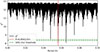 |
Fig. 1. Periodogram search for the sidereal rotation period. The horizontal axis shows the tested periods (0.40–0.50 h), and the vertical axis shows the corresponding χ2 values. Two periods within the χ2 threshold (defined by the dashed green line) were selected for further analysis. |
Instead of a single global minimum, two distinct local minima of a comparable depth were identified near 0.465 h and 0.456 h. Both candidate periods fall within the standard acceptance threshold of 10% above the global χ2 minimum (Hanuš et al. 2011). All other period candidates were rejected. The formal period uncertainty was estimated as one-twentieth of the width of the respective χ2 minima (Hanuš et al. 2011), yielding an uncertainty of approximately 1 × 10⁻⁶ h for both candidate solutions.
3.2. Bootstrap validation
To assess the robustness of the two period candidate solutions, we applied a bootstrap resampling procedure (Hanuš et al. 2015). We generated 700 synthetic datasets by resampling, with replacement, the photometric data and, at each iteration, we repeated the period scan over the restricted interval 0.45–0.47 h.
The resulting distribution (Fig. B.1) clusters around the two candidate minima, confirming that both are supported by the data. The P ∼ 0.456 h solution appears in ∼69% of realisations, indicating a statistical preference. However, given the limited number of apparitions and similar χ2 depths, we retain both periods for further analysis.
3.3. Spin-axis search
For each candidate rotation period, we performed an exploration of the spin-axis orientation by scanning the celestial sphere in ecliptic coordinates, using a grid with 15° spacing in both ecliptic longitude (λ) and latitude (β), corresponding to 312 trial pole directions. For each pole direction, the light-curve inversion was executed with the rotation period fixed to the candidate value, and the corresponding χ2 was recorded.
The resulting χ2 distribution over the sky reveals regions (dark areas of Fig. 2) of admissible solutions rather than isolated points. Following the criterion of Hanuš et al. (2011), we defined all solutions satisfying Δχ2/χmin2 < 0.1, where Δχ2 = χ2 − χmin2 are admissible solutions. Not unexpectedly, these solutions are enclosed in regions (white curves of Fig. 2) corresponding to local χ2 minima and they represent spin-axis orientations compatible with the data. This procedure was applied independently for both candidate periods. For the P = 0.465 h case, two dominant regions were found, forming a pair of mirror pole solutions separated by approximately 180° in longitude. This is the well-known ambiguity of light-curve inversion with limited viewing geometries.
 |
Fig. 2. Pole map obtained using the ‘medium’ search option of MPO LCInvert. Dark regions indicate the lowest χ2 values, while yellow regions indicate the highest. White lines contour the regions of admissible solutions (see Sect. 3.3). |
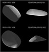 |
Fig. 3. Convex shape model (Solution 1 for the 0.465 h period). |
3.4. Final shape solution
For each candidate period (P ∼ 0.465 h and P ∼ 0.456 h) starting with the lower χ2 solution within each separate region of Δχ2/χmin2 < 0.1 identified by means of the method of Sect. 3.3, we performed a refined inversion in which both the rotation period and the spin-axis orientation were allowed to vary simultaneously. This step enables convergence towards the nearest local χ2 minimum within each region, allowing the pole, period, and shape model to be optimised, and this typically yields solutions with slightly lower χ2 values than those obtained in the fixed-period pole scan. Convergence to one local χ2 minimum per region was observed (Table 2).
Solutions at local minima within acceptable regions.
The resulting set of acceptable solutions, i.e. those within the white curves of Fig. 2, defines the uncertainty in the determination of the spin vector and rotation period. This approach gives a realistic estimate of the admissible region in spin-vector space given the data quality and observational geometry.
4. Results
The convex inversion analysis reveals two local minima in the explored period interval at P ∼ 0.465 h and P ∼ 0.456 h (Fig. 1, Table 2). For P ∼ 0.465 h, two pole solutions are found at (λ, β) = (126° , − 16° ) and (278° , − 28° ), with χ2 = 7.648 and 7.822, respectively. A third, less-preferable solution is also found at (λ, β) = (300° ,45° ) with χ2 = 7.844. For P ∼ 0.456 h, three additional solutions are obtained at (260° , − 39° ), (73° ,63° ), and (30° ,15° ), with χ2 values between 8.241 and 8.685. The formally preferred solution corresponds to P = 0.464982 h and (λ, β) = (126° , − 16° ), providing the lowest χ2 (7.648). The root mean square (RMS) of the residuals between the model and the data is 0.21 magnitudes, consistent with the expected photometric scatter (see Appendix A).
The proximity in χ2 between the two P ∼ 0.465 h solutions and their difference in λ suggests the typical ambiguity in pole determination arising from limited aspect-angle coverage. Nevertheless, the lowest χ2 solution is statistically favoured. Considering the extremely short rotation period (P ∼ 0.465 h), the shape does not exhibit an elongation sufficient to justify rotational stability solely through self-gravity. The object does not show evidence of extreme centrifugal deformation; therefore, its rotational stability is plausibly maintained by non-negligible internal cohesive strength, consistent with expectations for super-fast rotators and with the possibility that it may represent a fragment of lunar bedrock.
Overall, the derived shape model reproduces the observed photometric amplitudes well. The residual scatter of the fit is comparable to the typical photometric uncertainties, indicating that the reconstructed geometry adequately explains the observed brightness variations without requiring unrealistically extreme morphological features. Figure 2 presents the convex shape model associated with the preferred spin-state solution.
5. Discussion
All alternative solutions (Table 2) preserve the overall convex and elongated morphology of the preferred model. However, they differ in the distribution of volume along the principal axis. In particular, solution 2 with P ∼ 0.465 h mainly shows a moderate redistribution of volume without significantly altering the global elongation. Solution 3 with P ∼ 0.465 h appears elongated and flattened, with a protrusion at one end. Solution 1 with P ∼ 0.456 h appears more compact and less tapered, with a thicker central region and a more massive extremity; Solution 2 with P ∼ 0.456 h is very similar to the preferred solution. Solution 3 with P ∼ 0.456 h turns out to be flattened and quite angular. None of the models display bilobate features. For the figures corresponding to all the shapes, readers can refer to Appendix C.
The markedly elongated shape derived for Kamo’oalewa is difficult to reconcile with a purely hydrostatic equilibrium configuration, particularly given its extremely short rotation period. The absence of pronounced equatorial bulging or signatures of centrifugal mass redistribution suggests that the morphology is not the result of rotational deformation of a strengthless body. Instead, it reflects a structure dominated by internal cohesion.
A qualitative comparison with the unusual morphology reported by Bolin et al. (2025b) for 2024 YR4 indicates that strongly anisotropic shapes may arise in small bodies as a consequence of collisional fragmentation followed by rotational evolution. In this framework, the observed elongation of Kamo’oalewa may largely preserve the geometry of the original fragment, maintained by non-negligible material strength.
Given its peculiar quasi-satellite dynamical state and the spectroscopic evidence (Sharkey et al. 2021) pointing to a lunar origin, a plausible scenario is that Kamo’oalewa represents a fragment of lunar crust ejected during a high-energy impact on the Moon. This context could explain its current elongated morphology, which was subsequently preserved during its dynamical evolution within the Earth-Moon system.
Acknowledgments
Part of this work was supported by ESO, project number Ts 17/2–1. JH was supported by the Czech Science Foundation (grant 25-16789S). MD is supported by CNES and is Leverhulme Visiting Professor at the University of Leicester with financial support from the Leverhulme Trust (UK).
References
- Binzel, R. P., Rivkin, A. S., Stuart, J., et al. 2004, Icarus, 170, 259 [NASA ADS] [CrossRef] [Google Scholar]
- Bolin, B. T., Denneau, L., Abron, L.-M., et al. 2025a, ApJ, 978, L37 [NASA ADS] [CrossRef] [Google Scholar]
- Bolin, B. T., Hanuš, J., Denneau, L., et al. 2025b, ApJ, 984, L25 [Google Scholar]
- Bottke, W. F., Vokrouhlický, D., Rubincam, D. P., & Nesvorný, D. 2006, Annu. Rev. Earth Planet. Sci., 34, 157 [CrossRef] [Google Scholar]
- Chambers, K. C., Magnier, E. A., Metcalfe, N., et al. 2019, The Pan-STARRS1 Surveys [Google Scholar]
- Cheng, A. F., Agrusa, H. F., Barbee, B. W., et al. 2023, Nature, 616, 457 [NASA ADS] [CrossRef] [Google Scholar]
- Clark, B. E., Ziffer, J., Nesvorny, D., et al. 2010, JGR, 115, E06005 [Google Scholar]
- Connors, M., Wiegert, P., & Veillet, C. 2011, Nature, 475, 481 [CrossRef] [Google Scholar]
- Delbo’, M., dell’Oro, A., Harris, A. W., Mottola, S., & Mueller, M. 2007, Icarus, 190, 236 [CrossRef] [Google Scholar]
- Ďurech, J., Sidorin, V., & Kaasalainen, M. 2010, A&A, 513, A46 [Google Scholar]
- Elvis, M. 2013, in Asteroids: Prospective Energy and Material Resources, ed. V. Badescu, 81 [Google Scholar]
- Emery, J., Fernández, Y., Kelley, M., et al. 2014, Icarus, 234, 17 [NASA ADS] [CrossRef] [Google Scholar]
- Fenucci, M., Novaković, B., Vokrouhlický, D., & Weryk, R. J. 2021, A&A, 647, A61 [NASA ADS] [CrossRef] [EDP Sciences] [Google Scholar]
- Fujiwara, A., Kawaguchi, J., Yeomans, D. K., et al. 2006, Science, 312, 1330 [NASA ADS] [CrossRef] [Google Scholar]
- Hanuš, J., Ďurech, J., Brož, M., et al. 2011, A&A, 530, A134 [NASA ADS] [CrossRef] [EDP Sciences] [Google Scholar]
- Hanuš, J., Delbo’, M., Ďurech, J., & Alí-Lagoa, V. 2015, Icarus, 256, 101 [CrossRef] [Google Scholar]
- Hanuš, J., Delbo, M., Pokorný, P., Marchis, F., & Esposito, T. M. 2025, A&A, 704, A67 [NASA ADS] [CrossRef] [EDP Sciences] [Google Scholar]
- Hergenrother, C. W., Nolan, M. C., Binzel, R. P., et al. 2013, Icarus, 226, 663 [NASA ADS] [CrossRef] [Google Scholar]
- Kaasalainen, M. 2001a, Icarus, 153, 24 [NASA ADS] [CrossRef] [Google Scholar]
- Kaasalainen, M. 2001b, Icarus, 153, 37 [NASA ADS] [CrossRef] [Google Scholar]
- Lauretta, D. S., Balram-Knutson, S. S., Beshore, E., et al. 2017, Space Sci. Rev., 212, 925 [Google Scholar]
- Lauretta, D. S., Connolly, H. C., Aebersold, J. E., et al. 2024, Meteorit. Planet. Sci., maps.14227 [Google Scholar]
- Liu, L., Yan, J., Ye, M., et al. 2022, A&A, 667, A150 [NASA ADS] [CrossRef] [EDP Sciences] [Google Scholar]
- Nolan, M. C., Magri, C., Howell, E. S., et al. 2013, Icarus, 226, 629 [Google Scholar]
- Novaković, B., Fenucci, M., Marčeta, D., & Pavela, D. 2024, PSJ, 5, 11 [Google Scholar]
- Nugent, C. R., Andersen, K. P., Bauer, J. M., et al. 2025, PSJ, 6, 190 [Google Scholar]
- Perna, D., Barucci, M. A., & Fulchignoni, M. 2013, Astron. Astrophys. Rev., 21, 65 [Google Scholar]
- Sharkey, B. N. L., Reddy, V., Malhotra, R., et al. 2021, Commun. Earth Environ., 2, 231 [NASA ADS] [CrossRef] [Google Scholar]
- Vavilov, D. E., & Hestroffer, D. 2026, A&A, 707, A317 [NASA ADS] [CrossRef] [EDP Sciences] [Google Scholar]
- Veverka, J., Farquhar, B., Robinson, M., et al. 2001, Nature, 413, 390 [NASA ADS] [CrossRef] [Google Scholar]
- Warner, B. D. 2006, A Practical Guide to Lightcurve Photometry and Analysis (New York, NY, USA: Springer) [Google Scholar]
- Warner, B. D. 2012, MPO LCInvert: Lightcurve inversion software, Minor Planet Observer/MPO Software, available from the MPO software suite, see https://www.minorplanetobserver.com/MPOSoftware/MPOLCInvert.htm [Google Scholar]
- Warner, B. D., Harris, A. W., & Pravec, P. 2009, Icarus, 202, 134 [NASA ADS] [CrossRef] [Google Scholar]
- Watanabe, S., Hirabayashi, M., Hirata, N., et al. 2019, Science, 364, 268 [NASA ADS] [Google Scholar]
- Wiegert, P. A., Innanen, K., & Mikkola, S. 2000, AJ, 119, 1978 [NASA ADS] [CrossRef] [Google Scholar]
mp3c.le.ac.uk; version 3.0.0-beta.22 of 2026-03-06.
In 2025, China’s Tianwen-2 was launched to visit near-Earth asteroid Kamo’oalewa, (see SpaceNews, which was accessed on September 23, 2025.
Appendix A: Supplementary analysis
Information about the photometric uncertainties is not available from the AstDys repository. However, two different approaches can be used to estimate these uncertainties (Hanuš et al. 2011, see, e.g., and references therein). The first is to measure the RMS of the convex inversion fit, which we find to be 0.21 magnitudes, roughly reflecting the noise in the data. The second is to fit a Fourier curve to each light curve and compute the RMS. This yields values between 0.10 and 0.32 magnitudes, with an average of 0.23 magnitudes, which is very similar to the value obtained using the first method. Figure A.1 shows an example of the convex inversion model fit to a light curve.
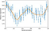 |
Fig. A.1. Example of a model fit to the observed light curve. Blue points with error bars correspond to the photometric measurements, assuming a 0.23 magnitude error, while the orange line shows the synthetic light curve derived from the shape model. Data are plotted as a function of rotational phase, and magnitudes are given as relative values. |
Appendix B: Supplementary figure
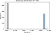 |
Fig. B.1. Bootstrap resampling of the photometric dataset. We show a histogram of the best-fitting periods – the two previously derived sidereal periods clearly dominate. The 0.456 h period is more common – in ∼69% cases. |
Appendix C: Shape model projections
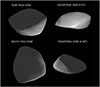 |
Fig. C.1. Convex shape model corresponding to solution 2 for the 0.465 h period of Kamo’oalewa. |
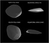 |
Fig. C.2. Convex shape model corresponding to solution 3 for the 0.465 h period of Kamo’oalewa. |
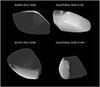 |
Fig. C.3. Convex shape model corresponding to solution 1 for the 0.456 h period of Kamo’oalewa. |
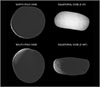 |
Fig. C.4. Convex shape model corresponding to solution 2 for the 0.456 h period of Kamo’oalewa. |
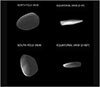 |
Fig. C.5. Convex shape model corresponding to solution 3 for the 0.456 h period of Kamo’oalewa. |
All Tables
All Figures
|
Fig. 1. Periodogram search for the sidereal rotation period. The horizontal axis shows the tested periods (0.40–0.50 h), and the vertical axis shows the corresponding χ2 values. Two periods within the χ2 threshold (defined by the dashed green line) were selected for further analysis. |
| In the text | |
|
Fig. 2. Pole map obtained using the ‘medium’ search option of MPO LCInvert. Dark regions indicate the lowest χ2 values, while yellow regions indicate the highest. White lines contour the regions of admissible solutions (see Sect. 3.3). |
| In the text | |
|
Fig. 3. Convex shape model (Solution 1 for the 0.465 h period). |
| In the text | |
|
Fig. A.1. Example of a model fit to the observed light curve. Blue points with error bars correspond to the photometric measurements, assuming a 0.23 magnitude error, while the orange line shows the synthetic light curve derived from the shape model. Data are plotted as a function of rotational phase, and magnitudes are given as relative values. |
| In the text | |
|
Fig. B.1. Bootstrap resampling of the photometric dataset. We show a histogram of the best-fitting periods – the two previously derived sidereal periods clearly dominate. The 0.456 h period is more common – in ∼69% cases. |
| In the text | |
|
Fig. C.1. Convex shape model corresponding to solution 2 for the 0.465 h period of Kamo’oalewa. |
| In the text | |
|
Fig. C.2. Convex shape model corresponding to solution 3 for the 0.465 h period of Kamo’oalewa. |
| In the text | |
|
Fig. C.3. Convex shape model corresponding to solution 1 for the 0.456 h period of Kamo’oalewa. |
| In the text | |
|
Fig. C.4. Convex shape model corresponding to solution 2 for the 0.456 h period of Kamo’oalewa. |
| In the text | |
|
Fig. C.5. Convex shape model corresponding to solution 3 for the 0.456 h period of Kamo’oalewa. |
| In the text | |
Current usage metrics show cumulative count of Article Views (full-text article views including HTML views, PDF and ePub downloads, according to the available data) and Abstracts Views on Vision4Press platform.
Data correspond to usage on the plateform after 2015. The current usage metrics is available 48-96 hours after online publication and is updated daily on week days.
Initial download of the metrics may take a while.