


| Issue |
A&A
Volume 710, June 2026
|
|
|---|---|---|
| Article Number | A14 | |
| Number of page(s) | 15 | |
| Section | Astrophysical processes | |
| DOI | https://doi.org/10.1051/0004-6361/202659871 | |
| Published online | 28 May 2026 | |
Acoustic instability at shockwave precursors
1
Gran Sasso Science Institute (GSSI), L’Aquila, Italy
2
INFN – Laboratori Nazionali del Gran Sasso (LNGS), L’Aquila, Italy
★ Corresponding author: This email address is being protected from spambots. You need JavaScript enabled to view it.
Received:
15
March
2026
Accepted:
13
April
2026
Abstract
Magnetic-field amplification is an integral part of the process of particle acceleration at nonrelativistic shocks. It is necessary to reach the maximum energies required by observations, especially in supernova remnants, which are thought to be sources of the majority of Galactic cosmic rays. Such amplification can be caused by the acoustic instability that develops when small density perturbations interact with the cosmic-ray pressure gradient upstream of a cosmic-ray-modified shock. The vorticity induced by the nonlinear development of the instability may lead to turbulence, which amplifies the preexisting magnetic fields. To study this phenomenon, we used the PLUTO code to carry out 2D (and some 3D) magnetohydrodynamical simulations of the evolution of small density perturbations in the presence of an assigned cosmic-ray pressure gradient. Adopting more realistic values of Mach number and cosmic-ray acceleration efficiency than previously assumed in the literature, we show that the acoustic instability can transform small density perturbations into large nonlinear structures, while the fluid crosses the precursor region of a cosmic-ray-modified shock. We studied the power spectrum of turbulent magnetic fluctuations that may be important to scatter particles. We comment on the possible constructive interference between acoustic and nonresonant streaming instabilities. We discuss limitations of previous and current numerical investigations in accessing spatial scales where turbulence is expected to turn nonlinear, and we outline perspectives for future investigations.
Key words: acceleration of particles / instabilities / magnetohydrodynamics (MHD) / shock waves / turbulence
© The Authors 2026
 Open Access article, published by EDP Sciences, under the terms of the Creative Commons Attribution License (https://creativecommons.org/licenses/by/4.0), which permits unrestricted use, distribution, and reproduction in any medium, provided the original work is properly cited.
This article is published in open access under the Subscribe to Open model. This email address is being protected from spambots. You need JavaScript enabled to view it. to support open access publication.
1. Introduction
The influence of cosmic rays (CRs) over their own transport is crucial to explain numerous phenomena, from the diffusive properties of astrophysical plasmas, to the maximum energy reached by accelerators and the subsequent spectra we measured at the Earth (see Blasi 2019 for a review of these effects). In recent decades, substantial progress has been made in understanding how CRs shape the environment in which they are produced. This is especially true for the vicinity of shockwaves, which are expected to be key sites of CR acceleration across a wide range of astrophysical settings, from supernova remnants (SNRs) (Blasi 2013; Amato 2014) to galaxy clusters (Blasi et al. 2007).
Despite the success of early theoretical approaches to diffusive shock acceleration (DSA), in which CRs were mostly treated as test particles (Krymskii 1977; Bell 1978), it soon became clear that to account for CRs up to the knee region or even higher energy CRs, efficient shock acceleration and strong magnetic fields–likely powered by CR-driven instabilities–were needed. In particular, the resonant streaming instability was invoked as a process responsible for magnetic-field amplification (MFA) upstream of nonrelativistic shocks (Skilling 1975; Bell 1978) and proven to lead to acceleration up to tens of teraelectronvolts in typical SNRs (Lagage & Cesarsky 1983). This process has the advantage of producing Alfvén waves on the right scale to scatter the same particles responsible for exciting the instability. On the other hand, the saturation of the instability to δB/B ≲ 1 implies that this process cannot account for particle acceleration to the knee. More recently, a nonresonant branch of the streaming instability (Bell 2004) received much attention: this instability is excited by the current induced by the CR particles escaping the upstream region of a shock and can lead to δB/B ≫ 1 due to its nonresonant nature. The instability is expected to saturate when particles start scattering on the self-generated perturbations. The implications of the excitation of the nonresonant modes in terms of the maximum energy of particles accelerated in SNR shocks have been discussed in a number of articles (Bell et al. 2013; Schure & Bell 2013; Cristofari et al. 2020, 2021). The consensus among these works is that although the instability appears to be very effective in amplifying the magnetic field on the relevant scales for very fast shocks in dense environments, the maximum energy at the beginning of the Sedov phase of SNRs typically falls short of a petaelectronvolt by at least one order of magnitude. This leaves open the possibility that other instabilities may lead to more effective MFA and perhaps more effective particle acceleration.
One such mechanism is associated with the pressure gradient that unavoidably forms upstream of a shock due to energy-dependent particle transport, which may induce the so-called Drury or acoustic instability (AI) in the presence of density inhomogeneities. This instability was first proposed by Drury (1984) and studied in detail by Drury & Falle (1986) (hereafter DF) using a two-fluid prescription in the absence of magnetic fields. This instability can overcome dissipation by CR diffusion (Ptuskin 1981) if the scale height of the CR pressure is smaller than the ratio between the local diffusion coefficient and sound speed, a condition naturally met at shockwave precursors. This results in an exponential growth of small inhomogeneities present in the interstellar medium (ISM) as they approach the shock surface. Numerical solutions to the equations in DF confirm the onset of the instability and the growth of density perturbations to nonlinear levels, if enough time is granted.
These findings have prompted further investigation of AI, especially in the context of CR-modified shocks (see Zank et al. 1990; Kang et al. 1992; Ryu et al. 1993; Begelman & Zweibel 1994; Webb et al. 1999, and references therein), although the nonlinear evolution of the system and the implications for MFA remain poorly understood. Beresnyak et al. (2009) proposed that the CR pressure gradient acting on large-amplitude density inhomogeneities upstream of a strong shock could induce turbulence, and that this might be reflected in higher maximum energies of the accelerated particles. In this picture, the solenoidal fluid motions act as a small-scale dynamo, amplifying magnetic fields by at least one order of magnitude via the stretch-twist-fold mechanism.
Drury & Downes (2012) (hereafter, DD) and Downes & Drury (2014) ran 2D magnetohydrodynamical (MHD) simulations of the precursor region, assuming that CRs were only responsible for the formation of an assigned pressure gradient. These simulations confirmed that MFA actually occurs. In 2D simulations, slightly more effective magnetic energy amplification is found, with a weak predominance of power on larger scales compared to the results of 3D simulations. More recently, del Valle et al. (2016) (hereafter, VLS) explored and expanded on this idea by means of 3D MHD simulations of SNR shock precursors. Their work provided quantitative insights into the development of small-scale dynamo, turbulence, and scales where equipartition between fluid and magnetic turbulence should be expected. We comment further on these results throughout this paper.
Much of this previous work is based on a few critical assumptions: the first is that a very large part (typically 60%) of the ram pressure is channeled into accelerated particles. Although early work on the nonlinear theory of DSA appeared to suggest that such an energy conversion efficiency would be feasible (Malkov & Drury 2001; Blasi 2002), later work, based on nonlinear DSA models (Morlino & Caprioli 2012) and simulations (Caprioli & Spitkovsky 2014), suggests a typical efficiency of ≲10%. The question of MFA in higher Mach numbers with more realistic shock precursors remains open. The second assumption is that the pre-existing density fluctuations in the upstream plasma are already relatively large: this leaves little room for AI, and in fact much of the previous work on the topic focused on the possibility that the CR pressure gradient may induce turbulence in an inhomogeneous plasma. Both of these assumptions were adopted in order to minimize the demands on the numerical machinery employed to simulate the instability.
In this work, we focused on three main goals: 1) providing an analytic framework to assess the importance of AI in the precursor in the presence of a magnetic field and confirming the linear evolution of the instability with 2D MHD simulations; 2) bridging the gap with previous work, by starting with small density perturbations and investigating the possibility that turbulence may be formed due to AI first and warping of the magnetic-field lines later; 3) using more realistic CR acceleration efficiencies and Mach numbers that are more appropriate to SNRs in the beginning of the Sedov phase (M∼ few hundreds). In this paper, we take special care to discuss the scales accessible to the simulations (namely with negligible numerical damping), in 2D and 3D, compared with the wavenumbers that are excited by AI.
This article is organized as follows. In Sect. 2, we present an analytic derivation of the dispersion relation and the growth rate of AI. We derived simple expressions for the maximum number of e-folds by which small upstream perturbations can grow before reaching the shock. In Sect. 3, we describe how we used a setup similar to that of DD to perform MHD simulations of the instability, comparing the observed growth rates with the expected ones obtained analytically. We also studied the nonlinear stage of the system, discuss MFA, and calculate the power spectrum of magnetic perturbations. Finally, in Sect. 4 we comment on the comparison between MFA due to the CR pressure gradient and the Bell instability, speculating about a possible cooperation between the two processes. We summarize our findings and present our conclusions in Sect. 5.
2. Acoustic instability
We considered a plasma with density ρ, velocity u, pressure P, adiabatic index γ, and magnetic field B. Since we aim to describe the plasma dynamics upstream of a nonrelativistic shock, where a CR pressure gradient is expected, the MHD equations should include a force term due to the presence of a CR pressure gradient, ∇PCR:
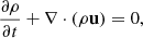 (1)
(1)
 (2)
(2)
 (3)
(3)
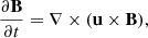 (4)
(4)
 (5)
(5)
Drury & Falle (1986) modeled the evolution of the CR pressure through the CR transport equation with diffusion coefficient D, and did not consider the effect of the magnetic field. By simultaneously perturbing ρ, u, P, and PCR, using a rigorous perturbative approach, they found that these perturbations grow when the length scale of the CR pressure gradient, PCR/∇PCR, is smaller than D/cs, where 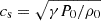 is the sound speed. If this condition is not met, the perturbations are damped due to friction with the CRs (Ptuskin 1981). In shock precursors, damping effects can be safely neglected because PCR/∇PCR ∼ D/vsh ≪ D/cs, where vsh ≫ cs is the shock speed. As such, for the case of a shock precursor, it is not necessary to go through the elegant but cumbersome calculations of DF, and the underlying physics describing the instability can be captured by perturbing only the plasma quantities ρ, u, and P, while assuming that ∇PCR is constant. Although this neglects the back-reaction of the instability onto CRs, it also reduces the complexity of the problem to a purely MHD one. We later comment on the implications of this assumption and on the reaction of the system to the enhanced scattering that may follow the excitation of the instability.
A clear advantage of the MHD formulation is that the dispersion relation and the growth rate of the instability can be derived straightforwardly. In the reference frame of the plasma, we can assume that the background plasma is uniform1 for Eqs. (1)–(5), with ρ = ρ0, u = 0, P = P0, and B = B0 while we introduce small perturbations–δρ, δu, δP, and δB–into the system. This approximation is valid for perturbations on scales much smaller than that of the CR pressure gradient. We assume that the perturbations are proportional to exp[i(k ⋅ x − ωt)]. The dispersion relation is
![Mathematical equation: $$ \begin{aligned} (\omega ^2 - v_{\rm A}^2k_\parallel ^2)&\left[\omega ^4 - \omega ^2\left(k^2c_{\rm ms}^2 + \frac{i\mathbf k \cdot \nabla P_{\rm CR}}{\rho _0}\right) \right.\nonumber \\&\qquad \left. + k^2k_\parallel ^2v_{\rm A}^2c_{\rm s}^2 + iv_{\rm A}^2k^2k_\parallel \frac{\partial _\parallel P_{\rm CR}}{\rho _0}\right] = 0, \end{aligned} $$](/articles/aa/full_html/2026/06/aa59871-26/aa59871-26-eq7.gif) (6)
(6)
where  is the Alfvén speed,
 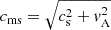 is the magnetosonic speed, and the ∥ subscript refers to components parallel to B0.
In addition to the usual Alfvén waves (ω2 = vA2k∥2), the dispersion relation shows that there are unstable modes obtained from roots of the expression inside the square brackets. When k∥ = 0, their dispersion relation is
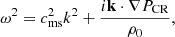 (7)
(7)
while for |k|=k∥ it is the same as in the absence of a magnetic field, namely
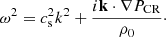 (8)
(8)
The growth rate of the instability, Γ, is characterized by two distinct regimes, which depend on the ratio between the real and imaginary parts of ω2. For example, Eq. (8) with k ∥ ∇PCR yields
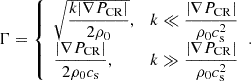 (9)
(9)
The real part of ω, which determines the phase velocity of the perturbations, is equal to Γ for long wavelengths (k ≪ |∇PCR|/ρ0cs2). Instead, the real part of ω is equal to csk for short wavelengths (k ≫ |∇PCR|/ρ0cs2). In the latter regime, the perturbations are modified sound waves, because Γ ≪ csk. In the other regime, the condition that the perturbations must occur on scales smaller than the size of the precursor, L ≈ PCR/∇PCR, implies that the sonic Mach number must be  , where ξCR = PCR/ρ0u02. This condition is certainly satisfied for shocks of astrophysical relevance.
To better understand the nature of the instability, we considered only modes with k ∥ ∇PCR and computed the eigenmodes of the system. If the density perturbation is given by δρ = δρ0 ei(k ⋅ x − ωt), one can show that pressure perturbations are δP = δρ0cs2 ei(k ⋅ x − ωt), just as in regular sound waves, while velocity perturbations become
 (10)
(10)
where ![Mathematical equation: $ \Omega = |\omega|=\sqrt[4]{c_s^4k^4 + (\mathbf{k}\cdot \nabla P_{\mathrm{CR}}/\rho_0)^2} $](/articles/aa/full_html/2026/06/aa59871-26/aa59871-26-eq15.gif) and ϕ = arg(ω2) = arctan(k ⋅ ∇PCR/ρ0cs2k2) is the principal value (−π/2 < ϕ ≤ π/2). The key point behind the instability is that velocity and pressure perturbations are out of phase, as was also noted in previous work (e.g., Begelman & Zweibel 1994). Consider only the positive sign of Eq. (10). Assuming k ⋅ ∇PCR = k|∇PCR| (i.e., ωR, ωI > 0), we have 0 < ϕ < π/2, and therefore the pressure lags the velocity in phase, which leads to instability. This is similar to pushing a swing soon after it starts moving away, increasing its amplitude of oscillation. Meanwhile, we find −π/2 < ϕ < 0 if we take waves in the opposite direction (k ⋅ ∇PCR = −k|∇PCR|, or equivalently ωR, ωI < 0), making pressure precede velocity in phase. The result is akin to pushing a swing too early, damping its motion. The equivalent analysis taking the negative sign for δu in Eq. (10) reverses the effects of leading/lagging pressure and is left for the reader to carry out.
and ϕ = arg(ω2) = arctan(k ⋅ ∇PCR/ρ0cs2k2) is the principal value (−π/2 < ϕ ≤ π/2). The key point behind the instability is that velocity and pressure perturbations are out of phase, as was also noted in previous work (e.g., Begelman & Zweibel 1994). Consider only the positive sign of Eq. (10). Assuming k ⋅ ∇PCR = k|∇PCR| (i.e., ωR, ωI > 0), we have 0 < ϕ < π/2, and therefore the pressure lags the velocity in phase, which leads to instability. This is similar to pushing a swing soon after it starts moving away, increasing its amplitude of oscillation. Meanwhile, we find −π/2 < ϕ < 0 if we take waves in the opposite direction (k ⋅ ∇PCR = −k|∇PCR|, or equivalently ωR, ωI < 0), making pressure precede velocity in phase. The result is akin to pushing a swing too early, damping its motion. The equivalent analysis taking the negative sign for δu in Eq. (10) reverses the effects of leading/lagging pressure and is left for the reader to carry out.
Figure 1 shows the real and complex parts of ω as functions of k, as predicted by Eqs. (7) and (8), along with their asymptotic behaviors. We assumed that k ∥ ∇PCR and the CR pressure gradient is constant, |∇PCR|=ξCRρ0u02/L, where L is the length of the precursor and ξCR is the fraction of the shock ram pressure converted into CRs. The number of e-folds available for the instability to grow on the precursor scale can be estimated as Γtadv, where tadv ≈ L/u0 is the advection timescale. In the absence of magnetic fields, Eq. (9) gives
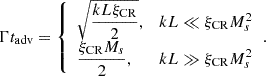 (11)
(11)
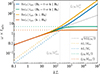 |
Fig. 1. Real and imaginary parts of ω. The CR pressure gradient is constant, |∇PCR|=ξCRρ0u02/L, and the perturbation wave vector, k, is aligned with ∇PCR. We assume ξCR = 0.1, Ms = 100, and |

The instability develops when Γtadv> a few. If the magnetic field is perpendicular to ∇PCR (and consequently to k), Ms should be replaced by the magnetosonic Mach number, Mms = u0/cms.
3. Simulations
In order to investigate the linear evolution of AI discussed in Sect. 2 and, more importantly, in order to study its nonlinear evolution, we performed MHD simulations using the PLUTO code (Mignone et al. 2007). Although most of our simulations are in 2D, we also compared the results of selected cases of physical interest with 3D simulations. Inspired by DD, our simulation box consists of a uniform 2D grid of dimensions Nx × Ny embedded in a Cartesian coordinate system with dimensions [0, L]×[0, L/8]. This region represents the precursor of a shockwave in the shock rest frame, with the shock itself lying just outside the right boundary at x = L. The x = 0 boundary represents upstream infinity (i.e., the ISM), where plasma of density ρ0, pressure P0, magnetic field B0, and adiabatic index γ = 5/3 enters the simulation box at the shock speed  .
.
The CR pressure gradient is introduced as a body force using the “VECTOR” prescription in PLUTO. For simplicity, we assumed that the CR pressure increases linearly from zero at x = 0 to a fraction, ξCR, of the shock ram pressure at x = L:
 (12)
(12)
The presence of ∇PCR induces nonuniform profiles along x in the density, velocity, pressure, and magnetic field of the background plasma. The steady-state profiles can be found by solving Eqs. (1)–(5) in their conservative form:
![Mathematical equation: $$ \begin{aligned} U(x)\equiv \frac{u(x)}{u_0}=\frac{\rho _0}{\rho (x)}=\left[\frac{P_0}{P(x)}\right]^{1/\gamma }=\frac{B_{y,0}}{B_y(x)} \end{aligned} $$](/articles/aa/full_html/2026/06/aa59871-26/aa59871-26-eq20.gif) (13)
(13)
and Bx(x) = Bx, 0, where U(x) satisfies
 (14)
(14)
where MA, y = u0/vA, y and  . Note that this is different from the Alfvénic Mach number MA = u0/vA.
Equation (14) can be solved numerically to find U(x) exactly. In the limit of high Mach numbers, one can approximate U(x)≈1 − ξCRx/L. The resulting density, velocity, pressure, and magnetic-field profiles are used as the initial conditions for the simulations. The time it takes for a fluid element entering from the left at x = 0 to reach a position x inside the box in the presence of a shock precursor is
 (15)
(15)
PLUTO implements boundary conditions (BCs) in each timestep by updating the value of physical quantities in inactive “ghost” cells surrounding the active Nx × Ny simulation grid. We used periodic BCs at the y = 0 and y = L/8 boundaries and an outflow (i.e., zero-gradient) BC at the x = L boundary, so that the plasma cannot flow back from the shock into the precursor. We extrapolated the variables into the ghost cells at x = 0 to avoid discontinuities of the derivatives. To avoid unphysical pressure waves that propagate back into the simulation box, we set the pressure at the right boundary to a very low value.
In Sect. 3.1, we used the “HLLC” Riemann solver with “MP5” reconstruction and third-order Runge–Kutta time-stepping (with Courant number CFL = 0.4 for 2D simulations and CFL = 0.3 for 3D simulations), while in Sect. 3.2 the solver and reconstruction were respectively downgraded to “HLL” and “PARABOLIC” for numerical stability purposes. The ∇ ⋅ B = 0 condition was controlled using the “CONSTRAINED_TRANSPORT” method under the “UCT_HLL” scheme. “ENTROPY_SWITCH” was always kept off.
3.1. The linear regime
We considered the linear regime where the perturbations produced by AI are much smaller than the unperturbed quantities in the entire simulation box. At x = 0, the BC was set to
 (16)
(16)
where 0 ≤ ϕ < 2π is a random phase,  , P = P0, and
  or
or  . Eq. (16) corresponds to a continuous inflow of density fluctuations with wavelengths λx = 2π/kx and λy = 2π/ky along the x and y directions. After one advection time, all transients due to initial conditions and boundary discontinuities at t = 0 disappear and the system reaches a quasi-stationary state. In Sects. 3.1.1 and 3.1.2 we study the behavior of kx modes (where ky = 0) and ky modes (where kx = 0) and test the growth rates of AI derived in Sect. 2. In Sect. 3.1.3 we investigate the more realistic scenario with many kx and ky modes.
3.1.1. Single kx mode
The simulations in this section were performed on a default grid resolution of Nx = 4000 and Ny = 4. The chosen value of Nx is large enough to avoid significant numerical damping. Since ∇PCR is oriented along the x-axis, density perturbations with ky = 0 are expected to induce δux, δP, and δBy perturbations that grow due to AI. In order to study the evolution of perturbations, we subtracted the background profiles from the total quantities provided as output by PLUTO, for example
 (17)
(17)
 (18)
(18)
To assess the validity of the analytic results derived in Sect. 2, we performed a scan over many different values of the parameters ξCR, Ms, δρ0/ρ0, vA/cs, and kxL = 2πλx−1L. In Fig. 2, we show some selected simulation results at steady state. Each subplot depicts constant-y slices of density (black), pressure (red), velocity (blue), and magnetic-field (green) perturbations, along with the corresponding expected growths ∝exp[Γt(x)] (dashed lines), which are all consistent with the simulation results2. In the top left panel, we adopted ξCR = 0.1, Ms = 100, δρ0/ρ0 = 10−4, kxL = 80π, and no background magnetic field, while in the bottom left panel we add a magnetic field perpendicular to the shock normal. As expected, a perpendicular magnetic field suppresses the growth rate of the instability. We also confirmed that a parallel field  reproduces the zero-field result. In the top right panel, we probe the small-wavelength limit (k ≳ |∇PCR|/ρ0cs2 = ξCRMs2/L), which requires a factor-ten increase in grid resolution (Nx = 40 000) to avoid numerical dissipation. Finally, in the bottom right panel, we consider larger values of δρ0/ρ0 and ξCR. In this case, the amplitude of the perturbations approaches the nonlinear regime close to the shock. As we discuss in Sect. 3.2, in this regime the perturbations steepen and eventually lead to the formation of shocklets.
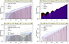 |
Fig. 2. Quasi-stationary x-profiles of the dimensionless density, pressure, velocity, and magnetic field perturbations from kx modes. We show the simulation results as solid lines and the expected growths for AI derived in Sect. 2 as dashed lines. In the bottom left panel, the initial magnetic field is pointed along y, and the lighter gray line corresponds to the expected growth in the absence of magnetic fields. |
3.1.2. Single ky mode
The dispersion relations given by Eqs. (7) and (8) show that only perturbation wave vectors parallel to ∇PCR lead to instability. However, perturbations with kx = 0 are also affected by the CR pressure gradient because the acceleration −∇PCR/ρ of a fluid element depends on the local density (overdensities decelerate slightly less than underdensities). For density perturbations along y, one has
 (19)
(19)
The first term corresponds to an overall deceleration of the fluid, while the second term leads to a relative acceleration of overdensities with respect to underdensities. The evolution of δux is given by (see Appendix A)
 (20)
(20)
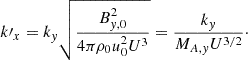
where
 (21)
(21)
Equation (20) can be interpreted as follows. Underdensities are more decelerated by the CR pressure gradient with respect to overdensities. Magnetic-field lines bend because they are frozen in the fluid, and magnetic tension acts as a restoring force. Then, δux oscillates while the fluid moves toward the shock. When there is no magnetic field, δux increases linearly.
This effect can be seen in Fig. 3, which shows the results of simulations performed on a grid with Nx = 2000 and Ny = 250. The top panels show the steady-state result of a simulation with the same parameters as in the top left panel of Fig. 2, but with a ky = 40π mode instead of a kx = 80π mode. On the left, we show δρ/ρ0. Sinusoidal oscillations along the y-axis do not grow exponentially, as expected. On the right, we show δux. We considered different y slices: y = ypeak (red), which is a peak of δρ/ρ0; y = ytrough (blue), which is a trough; and y = ynode (black), which is a node. The evolution also closely matches the prediction of Eq. (20) when By, 0 = 0; this is shown as dotted lines.
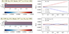 |
Fig. 3. Stationary profiles of dimensionless density (left) and velocity (right) perturbations from ky modes. On the right, red, blue, and black lines show the simulation results for δux/cs at a fixed y coordinate corresponding respectively to the peak, trough, and node of δρ/ρ0 oscillations. Dotted and dashed lines correspond to the analytical predictions of Eq. (20). Top: No magnetic fields. Bottom: Magnetic field perpendicular to the shock normal. |
The same quantities are shown in the bottom panels of Fig. 3, but for a different choice of parameters–notably with the addition of a perpendicular magnetic field such that vA = 3cs. The density profile looks qualitatively similar to the one in the top panel, indicating that no significant forces arise along the y direction. However, the velocity perturbations oscillate around zero, rather than growing linearly, because of magnetic tension. We verified the appearance of δBx in this simulation, thereby confirming our interpretation.
3.1.3. Many modes
We now address the more realistic case of ISM inhomogeneities across multiple scales and along all directions. The injected density profile is
![Mathematical equation: $$ \begin{aligned} \rho (x = 0,y,t)&=\rho _0\left[1 + \frac{\delta \rho _0}{\rho _0}(u_0 t,y)\right], \end{aligned} $$](/articles/aa/full_html/2026/06/aa59871-26/aa59871-26-eq34.gif) (22)
(22)
![Mathematical equation: $$ \begin{aligned} \frac{\delta \rho _0}{\rho _0}(x,y)&= \sum _{\begin{matrix} a,b = 0 \end{matrix}}^{N_x,N_y} A_{ab}\cos \left[\frac{2\pi }{L} (ax+by) + \phi _{ab}\right], \end{aligned} $$](/articles/aa/full_html/2026/06/aa59871-26/aa59871-26-eq35.gif) (23)
(23)
where Aab and ϕab are random amplitudes and phases of each perturbation. The latter are drawn uniformly from 0 ≤ ϕab < 2π, while the former were chosen so as to produce a flat omnidirectional power spectrum of ISM density fluctuations, Eδρ0/ρ0(k)∝k−1, with a root-mean-square (RMS) amplitude of δρ0, rms/ρ0 = 10−4. This procedure is described in Appendix B.1. Perturbations with wavelengths of > L/8 are set to have zero amplitude, while those with wavelengths down to grid-resolution scales are still injected into the system.
All power spectra in this work are calculated in the last eighth of the box (i.e., 7L/8 < x < L), since the amplitude of fluctuations is largest and nonlinear structures are most prominent in the part of the precursor that is closest to the shock. We also time-averaged the power spectra over several snapshots spanning one advection time, making them stationary.
Figure 4 shows the steady-state δρ/ρ0, δux, y, and δBx, y profiles (left) and the corresponding δρ/ρ0 power spectra (right), from a simulation performed in a 2048 × 256 grid using ξCR = 0.1, Ms = 100, and B0 directed along  such that vA = cs. The perturbations remain small before reaching the shock, while still growing exponentially at the nominal AI rate. Tracking the growth of each individual mode along the box becomes impractical, as it requires the use of sophisticated techniques such as wavelet transforms (Farge & Schneider 2015). Here, we adopted the simple Fourier transform (FT), whose formalism is outlined in Appendix B, sacrificing spatial resolution in order to obtain the power of each k mode averaged over the whole box.
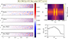 |
Fig. 4. Linear-regime simulation results for initial density fluctuations following Eq. (23) with a flat power spectrum in a 2048 × 256 grid. Left: Perturbation profiles for (from top to bottom) density, velocity x and y components, and magnetic-field x and y components. Note that δux/cs has been multiplied by 1/3 and δuy/cs by two, so all quantities can be visualized using the same color-bar scale. Right: Dimensionless 2D (top) and omnidirectional (bottom) density fluctuations’ power spectra, k2Pδρ/ρ0(kx, ky) and kEδρ/ρ0(k), respectively. |
The top right panel of Fig. 4 shows the 2D density power spectrum Pδρ/ρ0(kx, ky), multiplied by k2 to make it dimensionless. For k ≲ 103, the observed power spectrum resembles the expected AI growth rate. In other words, the amplitude of each (a, b) mode in Eq. (23) grows along the box as Aab(t) = Aabexp[Γ(ka, kb) t], where Γ(ka, kb) is the AI growth rate obtained from Eq. (6). Numerical damping significantly affects the simulation results for k ≳ 103, evidenced by a clear break at k ∼ 103 in the time-averaged omnidirectional power spectrum Eδρ/ρ0(k) shown in the bottom right panel. This is an unavoidable and critical feature of the simulations, which was also pointed out by DD and VLS.
3.2. Nonlinear regime
We considered the nonlinear regime where large perturbations are present near the shock surface (δρ, δP, δu, δB ≳ ρ0, P0, u0, B0). Large δB perturbations are expected to efficiently scatter particles, thus increasing their maximum energy. We show that AI can lead to large amplitude fluctuations even when the perturbations are small at upstream infinity.
We employed the simulation framework described in Sect. 3.1.3, injecting a superposition of perturbations down to the grid resolution scale. While the initial growth of preexisting small perturbations at upstream infinity is due to the onset of AI in the CR precursor pressure gradient, their nonlinear evolution is connected with the onset of turbulence. A similar investigation was carried out by DD using 2D MHD simulations and by VLS using 3D simulations. Both DD and VLS adopted parameters aimed at maximizing MFA, but that were not viable on physical grounds; for instance, the efficiency of particle acceleration was ξCR = 0.6, which is now considered disproportionately large with respect to the results of hybrid simulations, as well as phenomenological considerations, suggesting ξCR ≃ 0.1. In addition, previous studies considered Mach numbers of Ms ∼ 100, while shocks at the beginning of the Sedov phase of a SNR are expected to have Ms ∼ 500 and be even larger at earlier times.
The adoption of more realistic values of these parameters has profound consequences for MFA and for the onset of turbulence. In Fig. 5, we show 2D profiles of ρ/ρ0, ux, y/cs, Bx, y/B0, and (B/B0)2 for our benchmark choice of parameters (ξCR = 0.1, Ms = 500, δρ0, rms/ρ0 = 0.1, and vA = cs; left column), as well as for the parameters adopted in previous literature (ξCR = 0.6, Ms = 100, δρ0,rms/ρ0 = 0.1, and vA = cs; right column). The main qualitative differences are as follows: 1) the left profiles contain fluctuating structures predominantly on smaller scales with respect to the right profiles; 2) the amplitude of (δB/B0)2 fluctuations is smaller on the left, indicating a lower level of MFA; and 3) the combination of a longer advection time and a larger ξCR allows for early eddy formation in the right panels. Meanwhile, in the left panels, eddies form only very close to the shock, and most of the precursor is dominated by small-scale shocklets. Kang et al. (1992) suggested that these shocklets can play a role in energizing particles, even before they cross the shock surface. In both cases, the morphology of δBx is elongated along x, while δBy is elongated along y since the latter grows mainly due to plasma compression at the location of the shocklets.
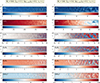 |
Fig. 5. Two-dimensional snapshots of quasi-stationary density, velocity, magnetic field, and magnetic energy density profiles, for different parameter choices, as indicated above each column, in a 4096 × 512 simulation grid. All quantities have been normalized so as to become dimensionless. For better contrast, color bars use linear scaling for ρ/ρ0 and ux/cs, logarithmic scaling for (B/B0)2, and symmetric logarithmic scaling (linear near zero and logarithmic at large amplitudes) for other quantities. |
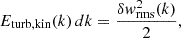
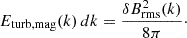
To quantitatively analyze our results, we calculated both kinetic and magnetic omnidirectional turbulent-energy-density spectra, Eturb, kin(k) and Eturb, mag(k), respectively, as defined in Appendix B. We first obtain the density-weighted velocity,  (as is customary in studies of compressible MHD turbulence; e.g., Kida & Orszag 1990; Grete et al. 2017), and the magnetic field, B(x, y), from the simulation output, and then subtracted their mean background profiles3
 and
and  to obtain the turbulent components:
 (24)
(24)
 (25)
(25)
The turbulent energy spectra are defined as the RMS energy density in turbulent fluctuations on scales between k and k + dk:
 (26)
(26)
 (27)
(27)
We also calculated the strength of MFA as a function of the distance from the shock surface:
 (28)
(28)
In Fig. 6, we show the turbulent power spectra and MFA for different choices of parameters (Ms, ξCR, vA/cs, δρ0,rms/ρ0, and magnetic-field orientation). In the top panels, we fix δρ0,rms/ρ0 = 0.1, vA = cs, and  while varying the remaining parameters. We compare the results for the benchmark values of the parameters (blue solid) with the DD/VLS parameters (dashed yellow) and with the more conservative case Ms = 100, ξCR = 0.1 (dotted green). It is worth recalling that for a typical SNR shock, the Mach number in the phase that is expected to be most important for particle acceleration is typically ∼100 − 1000 and the efficiency is ξCR ∼ 0.1. From the top-right panel we immediately see that the scenario with Ms = 100 and ξCR ∼ 0.1 does not yield any appreciable MFA; the background field still carries more energy than the fluctuations in this case. Note that in our benchmark case the turbulent magnetic-energy spectrum is very hard, with most of the power concentrated at small scales, which could translate into enhanced scattering of particles at the energies of interest (see discussion in Sect. 4). Meanwhile, strongly modified shocks with ξCR = 0.6 can easily produce δBrms/B0 ≳ 10, but their turbulent magnetic-energy spectra are somewhat steep, with most power concentrated on large scales. This is the only scenario in which we are anywhere close to reaching energy equipartition:
 (29)
(29)
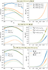 |
Fig. 6. Turbulent power spectra in units of ρ0cs2 (left) and MFA (right), calculated via Eq. (28), for different parameter values and a 4096 × 512 grid. Thick/thin lines in the left panels are kinetic/magnetic power spectra. The right panels’ legends indicate the colors/line styles corresponding to each choice of parameters. Top: We fix δρ0,rms/ρ0 = 0.1, vA = cs, and |


where  is the equipartition length scale. For smaller ξCR, the Mach number must be large to obtain any meaningful MFA. However, increasing the Mach number also increases Eturb, kin and keq. Ultimately, it is hard to estimate keq from simulations because this scale is never numerically resolved and Eturb, mag(k) does not follow the ∼k−1/2 scaling predicted by Beresnyak et al. (2009).
In the middle panels of Fig. 6 we instead fix Ms = 500 and ξCR = 0.1 and vary the remaining parameters while keeping  . For the dashed yellow curves, we set vA = 0.1cs, while for the dotted green curves, we doubled the RMS amplitude of the initial fluctuations, δρ0,rms/ρ0 = 0.2. Inspecting the low-k region of the power spectra, where numerical damping is negligible, we find that increasing vA by a factor of ten increases Eturb, mag by a factor of ≈100. Similarly, doubling δρ0,rms/ρ0 makes Eturb, mag larger by a factor of ≈4. This is consistent with the natural expectation that
  .
.
In the bottom panels we keep Ms, ξ, δρ0,rms/ρ0, and vA/cs fixed to their benchmark values to isolate the effect of field orientation. The results are somewhat consistent with the interpretation put forward by Downes & Drury (2014), the authors of which postulated that amplification occurs primarily to the component δBy. If the shock is parallel ( , dotted green lines), magnetic fluctuations along y arise only after the system turns nonlinear. Instead, if
  (solid blue lines), δBy is immediately generated in AI eigenmodes. The latter is the most optimistic scenario for MFA. However, more generally, SNR shocks expand onto oblique fields and MFA saturates between the two extreme cases discussed above. As an example, we show the case in which B0 is inclined by 30° with respect to the shock normal (dashed yellow lines). At low-k, its magnetic power spectrum is ∼4 times lower than the perpendicular shock case. This indicates that
  indeed dominates the amplified field.
To meaningfully interpret these results, in Fig. 7 we show a numerical convergence test, adopting the benchmark choice of parameters. In the left panel, we show the turbulent kinetic (thick lines) and magnetic (thin lines) power spectra, for different grid resolutions, normalized to ρ0cs2. The magnetic power peaks at larger k for higher resolution, but it is always far from reaching equipartition with the kinetic power. Note that doubling the grid resolution doubles the wavenumber, kd, above which damping is important (kdL ≈ 1.3 × 10³ for the 1024 × 128 resolution) and changes the shape of Eturb, mag(k) below kd, making it harder. This is not only due to the reduced numerical damping for k ≲ kd, it also happens because less power can be generated and transferred from higher to smaller k via inverse cascading. In the right panel, we show (δBrms/B0)2 as a function of x. As we can see, MFA increases with resolution, without converging. Our δB/B0 of order a few can only be interpreted as a conservative lower limit, because most of the magnetic energy is expected to be located at damping-dominated scales of kL ≳ 2000. As we show in Sect. 4, these scales play a crucial role in particle scattering.
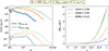 |
Fig. 7. Left: Turbulent kinetic (thick lines) and magnetic (thin lines) power spectra in units of ρ0cs2 for different grid resolutions (see right panel legend). Right: MFA as a function of x for different grid resolutions. |
In this work, we focused on 2D simulations in order to access smaller scales, which are the most important because they carry most of the turbulent magnetic energy. Both DD and VLS have shown that simulations in 2D yield less power on small scales than in 3D. This is likely because turbulent kinetic energy predominantly undergoes an inverse cascade in 2D and a forward cascade in 3D. However, for this difference to be appreciable, turbulence should develop and have enough time to transfer kinetic energy between scales. Energy can safely cascade from k1 → k2 when the eddy turnover time teddy(k)∼1/k δu(k) at all intermediate wavenumbers k1 < k < k2 is much shorter than the advection time in the precursor:
 (30)
(30)
The RMS amplitude of velocity fluctuations at a given k, δurms(k), is defined via Eδu(k) dk = ρ0δurms2(k)/2, where the velocity power spectrum, Eδu, is defined in Appendix B. Note that Eδu is different from Eturb, kin, which is defined in terms of  .
.
In Fig. 8, we compare power spectra (left panel), MFA (middle panel), and characteristic timescales (right panel) for our benchmark set of parameters and 1024 × 128 (×128) resolution, in 2D (blue solid lines) and 3D (yellow dashed lines) simulations, respectively. Indeed, we find slightly more kinetic power at higher k in the 3D scenario, as well as comparable MFA. However, numerical damping once again prevents us from resolving the scales in which this difference could become appreciable. By comparing the eddy turnover times in the right panel with the advection time (dotted green line), we see that condition (30) is only marginally satisfied, and significant energy cascading is not expected to take place. In contrast, using the overly optimistic ξCR = 0.6 and Ms = 100 adopted in DD and VLS, one expects stronger cascading simply because Γ tadv is larger in the kL ≪ ξCRMms2 limit, thus reaching the nonlinear/turbulent regime earlier. In summary, while 2D simulations allowed us to access perturbations with large wavenumbers, 3D simulations may provide a better description of the nonlinear phase if small scales are resolved. On the other hand, it is clear that accessing such scales in 3D simulations quickly becomes unbearably expensive from the computational point of view.
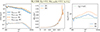 |
Fig. 8. Left: Turbulent kinetic (thick lines) and magnetic (thin lines) power spectra in units of ρ0cs2 for 2D (1024 × 128 grid; blue solid) and 3D (1024 × 128 × 128 grid; dashed yellow) simulations. Center: MFA as a function of x for 2D and 3D simulations. In 3D, we performed a yz averaging rather than just a y averaging. Right: Inverse eddy turnover timescales for the 2D (solid blue) and 3D (dashed yellow) runs, compared to the inverse advection timescale |

4. Competition and cooperation between acoustic and nonresonant instability
Particle acceleration at SNR shocks must be accompanied by substantial MFA, not only to reach a higher value of the maximum energy, but also to explain the thin filaments observed in X-rays (Vink 2012). It is, however, important to keep in mind that while the former point requires MFA upstream of the shock, namely in the CR precursor, to reduce the acceleration time, the latter only requires magnetic-field enhancement behind the shock.
All processes that can in principle lead to MFA are associated with a gradient in the CR distribution upstream: in the case of the nonresonant instability (Bell 2004), it is the current of particles escaping the upstream region that leads to the growth of the instability. In general, this phenomenon occurs on scales larger than the precursor size, which is L ∼ D(Emax)/vsh, where D is the diffusion coefficient and Emax is the maximum energy of the accelerated particles (for convenience, we use vsh rather than u0 in this section). Such current is directly related to the gradient of CR number density, and the process may lead to δB/B ≫ 1. For the resonant streaming instability (Lagage & Cesarsky 1983), it is the gradient of the CR density upstream to produce Alfvén waves at wavenumbers resonant with the CR momentum (rL(E)≃k−1). This latter process generally saturates at δB/B ≲ 1, especially if some type of damping is effective. Finally, AI discussed in this article grows due to the dynamical action of the CR pressure gradient upstream of the shock on density fluctuations present in the ISM and can lead to δB/B ≫ 1, depending on whether the instability has enough time to grow in one advection time. Below we comment on the location where these instabilities can be excited, on the scales involved and which one is expected to dominate as a function of the parameters.
If, for simplicity, we assume that the spectrum of accelerated particles is a power law in momentum space, f(p)∝p−4, which is appropriate for strong shocks, then the condition for the growth of the nonresonant instability can be written as
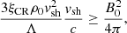 (31)
(31)
where Λ ≈ ln(Emax/mpc2)∼10. This condition is equivalent to requiring that the energy density carried by the current is larger than the energy density in the preexisting magnetic field (Bell 2004; Amato & Blasi 2009). If one introduces the Alfvénic Mach number in the preexisting field, then this condition can be rewritten as
 (32)
(32)
Typically, when the shock velocity drops below ∼1000 km/s, the nonresonant instability stops being excited and one has only the resonant streaming instability to rely upon.
At saturation, the magnetic field, Bsat, can be estimated from Eq. (31) by replacing B0 with Bsat and interpreting it as an equality. Following Schure & Bell (2013), Cristofari et al. (2020), the maximum energy is obtained by requiring that the instability grows for n e-folds, where typically it is assumed that n ≈ 5, namely γmaxt ≈ 5, where γmax is the maximum growth rate of the instability. When the nonresonant instability is excited, it is therefore driven by the current of escaping particles over a region with size  , where γmax = kmaxvA and
 (33)
(33)
is the scale where the growth is the fastest (Bell 2004). Here, JCR(> E) is the current carried by particles with energy > E. It can be easily shown that the condition in Eq. (31) is also equivalent to requiring kmax ≥ rL(E)−1, where rL(E) is the Larmor radius of the particles with energy E. The region affected by MFA, LMFA, is typically much larger than the size of the precursor, and the amplification of the magnetic field occurs on such a larger region. It is also important, for the considerations below, to keep in mind that the instability also results in overdensities of δρ/ρ0 ≳ 1 in the same region where the field is amplified.
At saturation, the nonresonant instability produces magnetic structures on the scale of the Larmor radius of the escaping particles in the amplified magnetic field. Using the considerations above, one finds that at the highest energy, Emax, the Larmor radius in the amplified field is
 (34)
(34)
At this point, the size of the precursor would be of the order of L ≃ D(Emax)/vsh, corresponding to a scale of 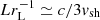 in the Bohm limit. For vsh = 103 − 104 km/s this corresponds to
  . Notice that these latter considerations apply to the nonresonant instability at saturation, while the wavenumber where the instability initially (in the linear regime) grows the fastest, kmax, corresponds to much smaller scales.
It is also useful to estimate L/Rsh, where Rsh is the radius of the shock, which is obtained by approximating vsht ≈ Rsh:
 (35)
(35)
For vsh = 103 − 104 km/s this corresponds to  , which is consistent with the typical approximation that D(Emax)/vsh ∼ 0.1Rsh.
The simple estimates presented here are formally valid for a parallel shock, although Bell (2005) showed that similar results are obtained for oblique shocks. Hence, we adopted the estimate of L provided above for oblique shocks as well. For shocks where the inclination to the shock normal is ≳45°, injection has been shown to be suppressed (Caprioli & Spitkovsky 2014), and they are of lesser interest here.
Let us now estimate these same quantities for AI. The fastest growing modes grow at a rate of ∼ξCRMmsvsh/2L, which is larger than the nonresonant growth rate at Emax when Mms ≳ (10/ξCR)(L/Rsh)∼10, where the last inequality holds if we adopt ξCR and L/Rsh ∼ 0.1. Based on these considerations, AI seems to grow faster for the high Mach number shocks that are typical of young SNRs.
As discussed above, the saturation of the instability is not easily accessible to current simulations; it requires the small-scale magnetic modes to reach some sort of equipartition with kinetic perturbations and initiate a nonlinear cascade toward larger scales. If trusting the qualitative expectations of DD, one could suggest that at saturation
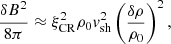 (36)
(36)
and assuming δρ/ρ0 ∼ 1 (which is the result of the nonlinear growth of the instability) we obtain the following ratio between the saturation values of the acoustic/turbulent to nonresonant instability:
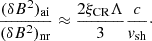 (37)
(37)
For typical values of the parameters, this ratio exceeds unity, which suggests that AI may prevail. As stressed above, numerical simulations of AI are not yet suitable to really test this regime and check the viability of Eq. (36).
We want to stress that the two CR-induced instabilities studied here may operate at the same time and in fact cooperate rather than compete with each other: the fact that the Bell instability operates due to the current of particles escaping the acceleration region implies that this instability produces density perturbations of δρ/ρ0 ≳ 1 upstream of a shock, over a region much larger than the size of the precursor. When these regions enter the shock precursor, they can undergo additional MFA due to the onset of AI and its nonlinear counterpart. However, this conclusion requires some caution; AI is expected to amplify the perpendicular component of the magnetic field, while, as discussed above, MFA is reduced in the case of parallel shocks. On the other hand, it is well known that the nonresonant instability creates large perpendicular magnetic fields away from the shock. Hence, by the time that these perturbations enter the precursor they can further be amplified by AI and the considerations above would apply.
While this synergic relation between the two processes can only be proven with dedicated simulations in which CRs are active components (hybrid or MHD+PIC simulations), it is worth stressing that hybrid simulations have already shown evidence for episodes in which particle trapping in large magnetic structures occurs upstream before these structures are eventually advected downstream (Zeković et al. 2025). It is possible that such structures may be the result of overdense regions being unstable in the CR pressure gradient.
5. Conclusions
Cosmic-ray-induced MFA is an integral part of the process of particle acceleration at shocks, especially in the case of SNR shocks. In this work we investigated the possibility that the amplification may be due to the reaction of small density perturbations to the CR pressure gradient in the upstream region of the shock, as originally suggested by DD. We expanded on previous investigations carried out using MHD simulations with an assigned pressure gradient (DD, VLS) by improving resolution, deepening the discussion around numerical damping and the role of dimensionality, and adopting parameter values that are closer to the ones expected for a realistic SNR shock.
Our conclusions can be summarized as follows. 1) AI can lead to the nonlinear growth of small perturbations even for initial perturbations of δρ/ρ0 ∼ 10−1. This phenomenon leads to considerable MFA, especially when the original field is perpendicular to the shock normal. In contrast, previous works started with large initial perturbations, so that the role of AI was somehow reduced and nonlinear effects started immediately. We provided expressions for the growth rate and the scales involved. 2) The detailed study of the dependence of our results on resolution showed that by increasing the resolution, more power appears at large wavenumbers, as expected based on AI, but even the highest resolution runs were incapable of properly resolving the small scales where equipartition of kinetic and magnetic power is expected, for the realistic values of ξCR and Mach number, Ms, adopted here. This consideration applies even more to previous investigations. As a consequence, we were only able to impose a lower limit to the magnitude of MFA. 3) When AI leads to δρ/ρ0 ≫ 1, we occasionally observe the formation of shocklets that temporarily stall and are later advected with the fluid across the shock. These structures look similar to the SLAMS known to the space plasma community (Schwartz et al. 1992) and may play an important role in particle acceleration. 4) For values of the Mach number appropriate for SNRs, we showed that AI may grow faster than the nonresonant instability and lead to a larger MFA. We comment on the possibility that Bell instability may cooperate by first creating regions with δρ/ρ0 ≳ 1 far upstream, and that these regions may induce further amplification due to the CR pressure gradient. Future investigation, possibly using an MHD+PIC approach, is planned to better study the nonlinear reaction of accelerated particles to this instability.
Acknowledgments
The authors are grateful to an anonymous referee for their comments that helped us improve the manuscript. They also acknowledge precious conversations with E. Amato, V. Berta, N. Bucciantini, D. Caprioli, B. Olmi. They are also thankful to L. Drury and T.P. Downes for clarifications on their earlier work. The work of PB and AC was partially funded by the European Union – Next Generation EU under PRIN-MUR 2022TJW4EJ “Unveiling the footprints of the cosmic ray journey through the Galaxy and beyond”. The work of PB was also partially funded under MUR National Innovation Ecosystem grant ECS00000041 – VITALITY/ASTRA – CUP D13C21000430001. The work of ES was supported by a Rita Levi Montalcini fellowship.
References
- Amato, E. 2014, Int. J. Mod. Phys. D, 23, 1430013 [CrossRef] [Google Scholar]
- Amato, E., & Blasi, P. 2009, MNRAS, 392, 1591 [Google Scholar]
- Batchelor, G. K. 1953, The Theory of Homogeneous Turbulence (Cambridge: Cambridge University Press) [Google Scholar]
- Begelman, M. C., & Zweibel, E. G. 1994, Astrophys. J., 431, 689 [Google Scholar]
- Bell, A. R. 1978, MNRAS, 182, 147 [Google Scholar]
- Bell, A. R. 2004, MNRAS, 353, 550 [Google Scholar]
- Bell, A. R. 2005, MNRAS, 358, 181 [NASA ADS] [CrossRef] [Google Scholar]
- Bell, A. R., Schure, K. M., Reville, B., & Giacinti, G. 2013, MNRAS, 431, 415 [Google Scholar]
- Beresnyak, A., Jones, T. W., & Lazarian, A. 2009, Astrophys. J., 707, 1541 [Google Scholar]
- Blasi, P. 2002, Astropart. Phys., 16, 429 [NASA ADS] [CrossRef] [Google Scholar]
- Blasi, P. 2013, A&ARv, 21, 70 [Google Scholar]
- Blasi, P. 2019, Galaxies, 7, 64 [Google Scholar]
- Blasi, P., Gabici, S., & Brunetti, G. 2007, Int. J. Mod. Phys. A, 22, 681 [NASA ADS] [CrossRef] [Google Scholar]
- Caprioli, D., & Spitkovsky, A. 2014, ApJ, 783, 91 [CrossRef] [Google Scholar]
- Cristofari, P., Blasi, P., & Amato, E. 2020, Astropart. Phys., 123, 102492 [Google Scholar]
- Cristofari, P., Blasi, P., & Caprioli, D. 2021, Astron. Astrophys., 650, A62 [Google Scholar]
- del Valle, M. V., Lazarian, A., & Santos-Lima, R. 2016, MNRAS, 458, 1645 [Google Scholar]
- Downes, T. P., & Drury, L. O. 2014, MNRAS, 444, 365 [Google Scholar]
- Drury, L. O. 1984, Adv. Space Res., 4, 185 [Google Scholar]
- Drury, L. O., & Downes, T. P. 2012, MNRAS, 427, 2308 [NASA ADS] [CrossRef] [Google Scholar]
- Drury, L. O., & Falle, S. A. E. G. 1986, MNRAS, 223, 353 [Google Scholar]
- Farge, M., & Schneider, K. 2015, J. Plasma Phys., 81, 435810602 [Google Scholar]
- Grete, P., O’Shea, B. W., Beckwith, K., Schmidt, W., & Christlieb, A. 2017, Phys. Plasmas, 24, 092311 [NASA ADS] [CrossRef] [Google Scholar]
- Harris, C. R., Millman, K. J., van der Walt, S. J., et al. 2020, Nature, 585, 357 [NASA ADS] [CrossRef] [Google Scholar]
- Kang, H., Jones, T. W., & Ryu, D. 1992, Astrophys. J., 385, 193 [Google Scholar]
- Kida, S., & Orszag, S. A. 1990, J. Sci. Comput., 5, 85 [NASA ADS] [CrossRef] [Google Scholar]
- Krymskii, G. F. 1977, Dokl. Akad. Nauk SSSR, 234, 1306 [NASA ADS] [Google Scholar]
- Lagage, P. O., & Cesarsky, C. J. 1983, Astron. Astrophys., 125, 249 [Google Scholar]
- Malkov, M. A., & Drury, L. O. 2001, Rep. Progr. Phys., 64, 429 [Google Scholar]
- Mignone, A., Bodo, G., Massaglia, S., et al. 2007, Astrophys. J. Suppl., 170, 228 [Google Scholar]
- Morlino, G., & Caprioli, D. 2012, Astron. Astrophys., 538, A81 [Google Scholar]
- Ptuskin, V. S. 1981, Astrophys. Space Sci., 76, 265 [Google Scholar]
- Ryu, D., Kang, H., & Jones, T. W. 1993, Astrophys. J., 405, 199 [Google Scholar]
- Schure, K. M., & Bell, A. R. 2013, MNRAS, 435, 1174 [NASA ADS] [CrossRef] [Google Scholar]
- Schwartz, S. J., Burgess, D., Wilkinson, W. P., et al. 1992, J. Geophys. Res., 97, 4209 [Google Scholar]
- Skilling, J. 1975, MNRAS, 173, 255 [NASA ADS] [CrossRef] [Google Scholar]
- Vink, J. 2012, A&ARv, 20, 49 [Google Scholar]
- Webb, G. M., Zakharian, A., & Zank, G. P. 1999, J. Plasma Phys., 61, 553 [Google Scholar]
- Zank, G. P., Axford, W. I., & McKenzie, J. F. 1990, Astron. Astrophys., 233, 275 [Google Scholar]
- Zeković, V., Spitkovsky, A., & Hemler, Z. 2025, ApJ, 988, 40 [Google Scholar]
Strictly speaking, one must introduce a balancing force, ∇PCR/ρ0, in order for this to be a solution of Eq. (2). Clearly, this term does not affect the perturbed equations.
An initial transient is present since we inject pure density perturbations, which are not eigenmodes of the instability. This transient is particularly visible in the top right and bottom left panels of Fig. 2. Once velocity/pressure/magnetic field fluctuations develop, the exponential growth becomes clear.
We calculated  and
and  by averaging each field component over the y (and z) direction(s) and over multiple snapshots in time, along an interval of tadv. This procedure ensures that δw and δB average to zero at each x.
We actually generate an isotropic δρ0/ρ0 field in 3D space with the desired power spectrum  , then take a 2D slice of it along the xy plane to be the injected field into the box. It can be shown that the 2D slice’s omnidirectional spectrum E2D(k⊥) obeys the same power law as the 3D one as long as α < 1.
Self-symmetric modes in which a = −a mod Nx and b = −b mod Ny must be real (Yab = 0) and are therefore sampled directly from a Gaussian distribution with zero mean and 2σab2 variance.
Appendix A: Velocity perturbations for ky modes
In this Appendix, we derive Eq. (20). We consider small density perturbations along y,
 (A.1)
(A.1)
We assume that the density perturbations are nearly independent of x, namely δρ ≃ δρ0 (see Fig. 3). The perturbed magnetic field is  , and the perturbed velocity is
  .
.
Since ξCR ≪ 1, the derivatives of U can be neglected with respect to the derivatives of the perturbations. Using ∇ ⋅ δB = 0, the steady-state induction equation, ∇ × (u × B) = 0, can be approximated as
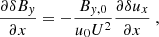 (A.2)
(A.2)
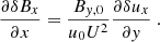 (A.3)
(A.3)
Assuming vA, y2 = By, 02/4πρ0 ≪ u02, and using Eq. (A.2), the momentum equation can be approximated as
 (A.4)
(A.4)
Making the ansatz δux = a(x)sin(kyy), Eq. (A.3) gives
 (A.5)
(A.5)
Taking the partial derivative of (A.4) with respect to x, we get
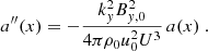 (A.6)
(A.6)
Solving Eq. (A.6) with BCs a(0) = 0 and a′(0) = (1/u0)(∇PCR/ρ0)(δρ0/ρ0) yields
 (A.7)
(A.7)
where kx′=ky(vA/u0)U−3/2.
Appendix B: Fourier transforms and power spectra
This Appendix outlines the formalism behind the discrete FT (DFT) and the power spectrum definitions used in Sect. 3. Below, f(x) denotes a generic field, representing density or a single velocity/magnetic field component. When specifically dealing with vector field components, we use Greek letter subscripts, f = (fα).
Our 2D simulation box has area A = L2/8 embedded within a grid of Ntot = NxNy points with uniform spacings along each direction, Δx = L/Nx and Δy = L/8Ny, and spatial coordinates
 (B.1)
(B.1)
This grid allows for specific wavenumbers along each direction:
 (B.2)
(B.2)
Grid cell areas are Δ2x = ΔxΔy and Δ2k = (2π)2/A in physical and reciprocal spaces, respectively. Note that, along each direction, the maximum allowed k corresponds to the Nyquist limit, kx, max = 2π/2Δx and ky, max = 2π/2Δy, while the minimum allowed k (besides the zero mode) corresponds to a wavelength the size of each box dimension, kx, min = 2π/L and ky, min = 2π/(L/8) = 16π/L.
We adopt the convention relating a two-dimensional field f(x) to its FT  via
via
 (B.3)
(B.3)
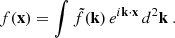 (B.4)
(B.4)
Upon discretization, this yields the DFT
 (B.5)
(B.5)
where one defines fij ≡ f(xij) and  , obeying Parseval’s identity
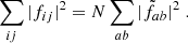 (B.6)
(B.6)
These DFTs can be efficiently calculated using NumPy’s ‘fft’ package (Harris et al. 2020) under the ‘forward’ normalization convention.
Under statistical homogeneity, the power spectrum tensor Pαβ(kab) is defined for vector fields via the ensemble average
 (B.7)
(B.7)
or, equivalently, as the FT of the correlation tensor
 (B.8)
(B.8)
Scalar fields yield a scalar power spectrum, P(kab), with an equivalent definition dropping the component indices. Rigorously performing ensemble averages requires many simulations, which is too computationally expensive. The best one can do from a single simulation is compute the estimator  , which is the FT of
  . Note that its trace at zero separation is
 (B.9)
(B.9)
We shall drop the hats from now on, always working with the estimators. For a statistically homogeneous and isotropic two-dimensional field satisfying ∇ ⋅ f = 0, one can write (Batchelor 1953)
 (B.10)
where  is the tensor’s trace, which depends only on k = |k|. For a scalar field, isotropy also implies that P(k) = P(k).
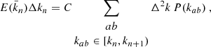
From P(kab) computed for either a scalar or a vector field f, one can define an omnidirectional power spectrum E(k) (also commonly called an “energy spectrum”) by binning k and adding all the power within each bin kab = |kab|∈[kn, kn + 1 = kn + Δkn):
 (B.11)
where  is a representative k in bin n (i.e. the geometric mean of its edges) and C is a constant prefactor depending on the specific field. This prefactor is introduced such that
  is an energy density, or some other quantity of interest, with
  being the contribution coming from bandwidth [kn, kn + Δkn]. In this work, we consider 4 types of omnidirectional power spectra:
-
For density fluctuations, the field is f = δρ/ρ0, and we choose C = 1 such that
![Mathematical equation: $$ \begin{aligned} \sum _n&E_{\delta \rho /\rho _0}(\bar{k}_n) \Delta k_n = \sum _{ab}\Delta ^2 k \, P(k_{ab}) = \xi (\mathbf 0 ) \nonumber \\&= \frac{1}{A}\sum _{ij}\Delta x \Delta y\,\left[\frac{\delta \rho }{\rho _0}(\mathbf x _{ij})\right]^2 = \left(\frac{\delta \rho _{rms}}{\rho _0}\right)^2\ , \end{aligned} $$](/articles/aa/full_html/2026/06/aa59871-26/aa59871-26-eq100.gif) (B.12)
(B.12)where δρrms/ρ0 is the RMS δρ/ρ0 over all scales in the box.
-
For magnetic fields fluctuations, f = δB, we choose C = 1/8π whereby the turbulent magnetic energy density power spectrum EδB(k)≡Eturb, mag(k) satisfies
 (B.13)
is the average magnetic energy density in perturbations at all scales, while
 is that coming from perturbations with wavenumbers k ∈ [kn, kn + Δkn]. In other words,
 (B.14)
is the RMS value of magnetic field fluctuations with characteristic scale
 .
. -
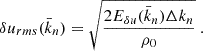
For velocity fields, e.g.δu, we choose C = ρ0/2 such that
 (B.15)
Analogously to the magnetic field case, the RMS amplitude of velocity perturbations at a characteristic scale
 can be found through
 (B.16)
 -
For studies of compressible turbulence, it is common to consider the density-weighted velocity
 to define kinetic energy spectra (Kida & Orszag 1990; Grete et al. 2017). Let δw be its fluctuations around a mean background profile. We can then choose C = 1/2 such that its corresponding power spectrum Eδw(k)≡Eturb, kin(k) is the turbulent kinetic energy spectrum:
 (B.17)
In practice, we calculate each E(k) by defining 50 logarithmically spaced k-bins between kmin = max(kx, min, ky, min) and kmax = min(kx, max, ky, max), and add their power following Eq. (B.11). This leads to
 (B.18)
with ln(kmax/kmin)/50 ≈ 0.1 in our simulations. This means that δBrms(k) and δurms(k) can be estimated, within factors of order unity, from the logarithmic energy spectrum kE(k) via:
 (B.19)
 (B.20)
Generating Initial Density Perturbations
In Sects. 3.1.3 and 3.2, we inject a density perturbations field δρ0(x)/ρ0 which is superposition of modes with different wave vectors, according to Eq. (23), following a predetermined omnidirectional power spectrum (with C = 1) between max(kx, min, ky, min) < k < min(kx, max, ky, max),
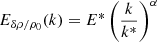 (B.21)
and zero outside this range, where E* is a normalization setting the power in fluctuations at a reference scale 2π/k*. We fix k* = min(kx, max, ky, max). Using the formalism presented above, we now describe our method for generating such a field4. This is done mode by mode in Fourier space, rather than directly in physical space, since it makes the connection with the desired power spectrum more direct.
We consider density perturbations to be Gaussian in nature, meaning that  , with Xab and Yab randomly sampled from a Gaussian distribution with zero mean and variance σab2. Writing this in polar form,
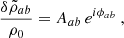 (B.22)
it can be easily shown that Aab follows a Rayleigh distribution with scale parameter σab, implying  , while ϕab is uniformly distributed between [0, 2π). Recall that producing a real δρ(xij)/ρ0 requires
  . This allows us to generate only half of the k-modes; once we have
  for all a, b ≥ 0, the modes with a, b < 0 are all set by the reality condition5: A−a, −b = Aab and ϕ−a, −b = −ϕab.
The power spectrum resulting from Eq. (B.22) is P(kab) = Aab2/Δ2k, while its inverse FT yields
 (B.23)
in agreement with Eq. (23). The RMS density perturbation over all scales can be be shown to match our expectation:
![Mathematical equation: $$ \begin{aligned} \left(\frac{\delta \rho _{\rm rms}}{\rho _0}\right)^2 =\frac{1}{N}\sum _{ij}\left[\frac{\delta \rho }{\rho _0}(\mathbf x _{ij})\right]^2 = \sum _{ab}A_{ab}^2 = E^*\sum _n \left(\frac{\bar{k}_n}{k^*}\right)^\alpha \Delta k_n\ . \end{aligned} $$](/articles/aa/full_html/2026/06/aa59871-26/aa59871-26-eq120.gif) (B.24)
(B.24)
Crucially, Eq. (B.24) allows us to find E* for any desired value of δρrms/ρ0. Meanwhile, the RMS value of perturbations on a scale kab is simply Aab, rms. The power inside each k-bin is
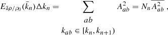 (B.25)
where  is the number of grid points in the bin and
  is the bin-averaged power per mode, which we set to Aab, rms. In the Δkn → 0 limit, this approaches
 (B.26)
This relation determines σab used to randomly sample each Aab mode, guaranteeing that the resulting spectrum will be properly normalized and follow the desired scaling with k. Once we have sampled every  , we simply take its inverse FT to get the final δρ(xij)/ρ0 entering the precursor.
All Figures
|
Fig. 1. Real and imaginary parts of ω. The CR pressure gradient is constant, |∇PCR|=ξCRρ0u02/L, and the perturbation wave vector, k, is aligned with ∇PCR. We assume ξCR = 0.1, Ms = 100, and |
| In the text | |
|
Fig. 2. Quasi-stationary x-profiles of the dimensionless density, pressure, velocity, and magnetic field perturbations from kx modes. We show the simulation results as solid lines and the expected growths for AI derived in Sect. 2 as dashed lines. In the bottom left panel, the initial magnetic field is pointed along y, and the lighter gray line corresponds to the expected growth in the absence of magnetic fields. |
| In the text | |
|
Fig. 3. Stationary profiles of dimensionless density (left) and velocity (right) perturbations from ky modes. On the right, red, blue, and black lines show the simulation results for δux/cs at a fixed y coordinate corresponding respectively to the peak, trough, and node of δρ/ρ0 oscillations. Dotted and dashed lines correspond to the analytical predictions of Eq. (20). Top: No magnetic fields. Bottom: Magnetic field perpendicular to the shock normal. |
| In the text | |
|
Fig. 4. Linear-regime simulation results for initial density fluctuations following Eq. (23) with a flat power spectrum in a 2048 × 256 grid. Left: Perturbation profiles for (from top to bottom) density, velocity x and y components, and magnetic-field x and y components. Note that δux/cs has been multiplied by 1/3 and δuy/cs by two, so all quantities can be visualized using the same color-bar scale. Right: Dimensionless 2D (top) and omnidirectional (bottom) density fluctuations’ power spectra, k2Pδρ/ρ0(kx, ky) and kEδρ/ρ0(k), respectively. |
| In the text | |
|
Fig. 5. Two-dimensional snapshots of quasi-stationary density, velocity, magnetic field, and magnetic energy density profiles, for different parameter choices, as indicated above each column, in a 4096 × 512 simulation grid. All quantities have been normalized so as to become dimensionless. For better contrast, color bars use linear scaling for ρ/ρ0 and ux/cs, logarithmic scaling for (B/B0)2, and symmetric logarithmic scaling (linear near zero and logarithmic at large amplitudes) for other quantities. |
| In the text | |
|
Fig. 6. Turbulent power spectra in units of ρ0cs2 (left) and MFA (right), calculated via Eq. (28), for different parameter values and a 4096 × 512 grid. Thick/thin lines in the left panels are kinetic/magnetic power spectra. The right panels’ legends indicate the colors/line styles corresponding to each choice of parameters. Top: We fix δρ0,rms/ρ0 = 0.1, vA = cs, and |
| In the text | |
|
Fig. 7. Left: Turbulent kinetic (thick lines) and magnetic (thin lines) power spectra in units of ρ0cs2 for different grid resolutions (see right panel legend). Right: MFA as a function of x for different grid resolutions. |
| In the text | |
|
Fig. 8. Left: Turbulent kinetic (thick lines) and magnetic (thin lines) power spectra in units of ρ0cs2 for 2D (1024 × 128 grid; blue solid) and 3D (1024 × 128 × 128 grid; dashed yellow) simulations. Center: MFA as a function of x for 2D and 3D simulations. In 3D, we performed a yz averaging rather than just a y averaging. Right: Inverse eddy turnover timescales for the 2D (solid blue) and 3D (dashed yellow) runs, compared to the inverse advection timescale |
| In the text | |
Current usage metrics show cumulative count of Article Views (full-text article views including HTML views, PDF and ePub downloads, according to the available data) and Abstracts Views on Vision4Press platform.
Data correspond to usage on the plateform after 2015. The current usage metrics is available 48-96 hours after online publication and is updated daily on week days.
Initial download of the metrics may take a while.