


| Issue |
A&A
Volume 710, June 2026
|
|
|---|---|---|
| Article Number | L2 | |
| Number of page(s) | 5 | |
| Section | Letters to the Editor | |
| DOI | https://doi.org/10.1051/0004-6361/202659819 | |
| Published online | 25 May 2026 | |
Letter to the Editor
Equilibrium figure of Haumea and possible detection via stellar occultation
1
Université Paris Cité, CNRS, Institut de Physique du Globe de Paris, F-75005, Paris, France
2
Sorbonne Université, Observatoire de Paris, Université PSL, CNRS, Laboratoire Temps Espace, F-75014, Paris, France
3
Université de Lyon, CNRS, ENS Lyon, Laboratoire de Géologie de Lyon Terre – Planètes – Environnement, F-69007, Lyon, France
4
Jet Propulsion Laboratory, California Institute of Technology, Pasadena, California, USA
★ Corresponding author: This email address is being protected from spambots. You need JavaScript enabled to view it.
Received:
12
March
2026
Accepted:
29
April
2026
Abstract
We studied the equilibrium figure of dwarf planet Haumea to determine if the observed shape is compatible with a differentiated hydrostatic body. Three groups of interior models of Haumea were assumed, all with a rocky core and a volatile-rich outer shell that may contain some porosity. A third layer located between the core and the outer shell has a density suggesting partial differentiation or the presence of a large fraction of organic matter. Using the code BALEINES, which solves for the equilibrium figures of the boundaries between layers, we show that the hydrostatic models closest to the shape derived via stellar occultation approach a state of critical rotation, which translates into a pinched shape with large deviations from an ellipsoid (up to 110 km). The previous stellar occultation and light curves cannot be used to distinguish between the ellipsoid and the pinched shape, but we predict this figure could be observable during the next stellar occultation of Haumea on May 4, 2026, if some chords are obtained in the northern or southern limbs of the shadow.
Key words: gravitation / methods: numerical / planets and satellites: interiors / Kuiper belt objects: individual: (136108) Haumea
© The Authors 2026
 Open Access article, published by EDP Sciences, under the terms of the Creative Commons Attribution License (https://creativecommons.org/licenses/by/4.0), which permits unrestricted use, distribution, and reproduction in any medium, provided the original work is properly cited.
This article is published in open access under the Subscribe to Open model. This email address is being protected from spambots. You need JavaScript enabled to view it. to support open access publication.
1. Introduction
(136108) Haumea is a rapidly rotating Kuiper belt object whose triaxial figure was derived by Ortiz et al. (2017) from a stellar occultation together with light curves. However, Kondratyev & Kornoukhov (2018) and Dunham et al. (2019) noted that this estimation assumed the occultation happened when Haumea’s brightness was at a minimum, whereas a rotational phase of −13.3° was observed; this phase difference changes the set of ellipsoids that are compatible with the projected ellipse. In both cases, the resulting best-fit ellipsoids are incompatible with a Jacobi ellipsoid, i.e. a homogeneous ellipsoid in hydrostatic equilibrium (see Fig. 1). This discrepancy implies that either rigid-body forces provide significant support against self-gravity or Haumea has undergone differentiation and is thus heterogeneous. Regarding the latter perspective, Dunham et al. (2019) and Noviello et al. (2022) studied two-layer hydrostatic models of Haumea, with a rocky core and an icy mantle. Their preferred model is nearly ellipsoidal and compatible with the chords of the 2017 occultation, meaning that Haumea can be consistent with differentiated hydrostatic bodies.
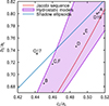 |
Fig. 1. Possible hydrostatic models obtained in this work (pink region). The models listed in Table 1 are plotted with black crosses. For reference, the Jacobi sequence is plotted as a red line. The best-fit ellipsoids from Ortiz et al. (2017, ‘O17’) and the hydrostatic model preferred by Dunham et al. (2019, ‘D19’) are reported with open circles. The ‘shadow ellipsoids’ curve corresponds to ellipsoids whose projection corresponds to the ellipse determined during the 2017 occultation, with the pole orientation obtained by Ortiz et al. (2017) and a rotational phase of −13.3°; see Drummond et al. (1985) for the equations used. Note that this curve is valid only for ellipsoidal shapes. |
A new stellar occultation by Haumea is predicted for May 4, 2026 (Ortiz et al. 2026)1, which may allow us to refine the observational constraints on its shape. Therefore, this Letter investigates triaxial equilibrium figures of two- and three-layer hydrostatic bodies to determine whether only nearly ellipsoidal shapes are likely to be observed. Unlike previous works, we show that, if Haumea has a hydrostatic shape, then it may deviate significantly from an ellipsoid and could even be pinched at the end of its equatorial major axis, indicating a state of critical rotation. Finally, we question whether observational data from May 2026 can be used to discriminate an ellipsoid from a pinched figure.
2. Hydrostatic shape models
The theory of equilibrium figures states that a rigidly rotating fluid mass is in hydrostatic equilibrium if and only if the surfaces of constant density and the surfaces of constant effective potential, i.e. the sum of the centrifugal and self-gravitational potentials, coincide (e.g. Zharkov & Trubitsyn 1978; Lanzano 1982). Determining an equilibrium figure then comes down to finding shapes of the fluid whose effective potential is constant on these surfaces. As the potential depends non-trivially on the shape, the corresponding equation set actually forms a fixed-point problem. In this Letter we consider a differentiated body composed of L = 2 or 3 homogeneous layers, indexed by ℓ with ℓ = 1 denoting the innermost layer and ℓ = L the outermost. Assuming homogenous layers is sufficient since, under the low pressures inside Haumea (≲500 MPa), the densities of ices and rocky minerals increase only by a few percent (the bulk moduli are ∼10 GPa for ices and ≳100 GPa for rocks).
We used the code BALEINES (Staelen & Huré 2026), which iteratively computes the shapes of the interfaces. Each surface is expanded over Chebyshev polynomials both for latitude and longitude, the potential is written in terms of surface integrals only, and these integrals are computed with Clenshaw-Curtis quadrature. Mirror symmetry with respect to the plane (xOy) is imposed by the Lichtenstein theorem, and mirror symmetry with respect to the planes (yOz) and (zOx) is assumed to reduce the computation times; O is the centre of mass, and (Ox), (Oy), and (Oz) coincide with its equatorial major, equatorial minor, and polar axes, respectively. We used 17 Chebyshev nodes for both the latitude and longitude, which results in a relative precision of the order of 10−4.
Here aℓ, bℓ, and cℓ are the equatorial major semi-axis, the equatorial minor semi-axis, and the polar axis of the boundary of layer ℓ; ρℓ is its mass density. The explored parameters of the models reported in this work are cL/aL, ρℓ/ρℓ + 1 (1 ≤ ℓ < L), and cℓ/cL. Starting from two- and three-layer models of Haumea, we explored a large range of this parameter space: ρℓ/ρℓ + 1 ∈ [1.2, 4.2], c1/c2 ∈ [0.25, 0.95] for two layers, c2/c3 ∈ [0.30, 0.95] and c1/c3 ∈ [0.25, c2/c3[ for three layers, and cL/aL ∈ [0.42, 0.52]. The results are summarised in Fig. 1, which displays, in the (cL/aL, bL/aL) plane, the region where hydrostatic models have been found. As expected, heterogeneity expands the possible ranges of bL/aL for a given cL/aL, while only a unique value is permitted in the homogeneous case. The hydrostatic figures are contained between two curves into the (cL/aL, bL/aL) plane: the curve at higher cL/aL is given by models with a large outer layer (Staelen & Huré 2026), while the curve at lower cL/aL corresponds to configurations at the mass-shedding limit. In other words, the centrifugal acceleration, Ω2aL (where Ω is the rotation rate) exactly balances the self-gravity at the end of the equatorial major axis, ga. To measure the proximity to this limit, we defined q = Ω2aL/|ga| so that the mass-shedding limit, or critical rotation, is defined by q = 1.
3. Compatibility with the observational data
All quantities in BALEINES are normalised by the length of the equatorial major semi-axis and the mass density of the outermost layer of the fluid mass, aL and ρL. To compare the outputs with data, we had to revert to dimensional quantities. These physical outputs were obtained by requiring that the mass match the value currently determined for Haumea, i.e. M = 3.952 × 10²¹ kg (Proudfoot et al. 2024), and that the length of the minor equatorial semi-axis (bL) equal 840 km (Dunham et al. 2019). We imposed bL since it is the best constrained semi-axis length, with estimated values between 830 ± 6 km (Kondratyev & Kornoukhov 2018) and 852 ± 4 km (Ortiz et al. 2017). We conducted tests using both these lengths, and neither result differed significantly from the value chosen here.
From the explored space, we selected six configurations, labelled A to F, whose free surface shapes are coherent with the chords obtained during the 2017 occultation event. Figure 2 shows that their boundaries are quite elliptical in the (yOz) plane but deviate significantly from an ellipse in the (xOz) plane, up to a pinched shape for configurations B, C, and F. The maximal deviations from an ellipsoid are approximatively 110 km for the pinched configurations. The properties of these six configurations are reported in Table 1 and Fig. 1.
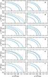 |
Fig. 2. Hydrostatic shape models for Haumea in the (xOz) (left) and (yOz) (right) planes, corresponding to the configurations reported in Table 1. The dashed lines correspond to the ellipsoids with the same axis lengths as the layers’ boundary. |
Examples of hydrostatic solutions whose free surface is coherent with the chords obtained during the 2017 occultation (Ortiz et al. 2017).
We also projected their free surface onto the sky plane at the epoch of the 2017 occultation; see Fig. 3. To do so, we used the Chebyshev expansion to resample the shape of the free surface and formed a regular triangular mesh with 15155 facets, which we used as an input file for the open-access tool developed by Rizos et al. (2025). These projections confirm that hydrostatic models are able to fit the occultation chords obtained by Ortiz et al. (2017). Light curves obtained with these shapes are reported in Appendix A and show that hydrostatic models are also able to fit the light curves obtained by Lacerda et al. (2008), Lockwood et al. (2014), and Ortiz et al. (2017). Finally, the J2 values of these configurations are compatible with the corresponding observation: they vary from 0.140 to 0.159, and this range lies near the bottom of the 1σ confidence region obtained by Proudfoot et al. (2024) via orbit fitting, i.e.  .
.
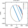 |
Fig. 3. Projections of the six hydrostatic representative solutions in the sky plane at the epoch of the 2017 occultation. u and v are celestial east and north, respectively. The pole orientation is the one obtained by Ortiz et al. (2017), and the rotational phase is −13.3°. |
4. Discussion
4.1. Haumea as a critical rotator
Some hydrostatic figures exhibit a pinched geometry, i.e. the surface normal becomes discontinuous at the end of the major equatorial axis. Since the effective gravity is continuous and, for a hydrostatic body, orthogonal to the equipotential surfaces, this behaviour is possible only if the effective gravity vanishes at that point, i.e. for critical rotators (q = 1). This is illustrated by configurations B, C, and E, whose values of q, reported in Table 1, are between 0.96 and 0.99. It is noteworthy that pinched shapes for critical rotators are actually well documented in the context of stellar physics (e.g. Maeder & Meynet 2012). Furthermore, such equatorial ridges have been observed in several fast-rotating asteroids, including (2867) Šteins (Jorda et al. 2012) and (65803) Didymos (Barnouin et al. 2024). We also note that even configuration D is close to the mass-shedding limit (q = 0.73, which corresponds to 85% of the critical rotation rate). Critical rotators are closer to the observed rotation period as c/a approaches 0.45 (configuration B), while for c/a ≳ 0.49, only figures close to ellipsoids are compatible to the rotation period (configurations A and E).
4.2. Haumea’s shape as a fossil figure
As shown by configurations A, B, and D, some models are fully compatible with the 2017 occultation and the observed rotation period of Haumea. However, Haumea’s shape could also be ‘frozen’, i.e. representative of a previous rotation state, and, if so, would then depart from hydrostatic equilibrium; this is why we have not imposed that our models exactly fit the observed rotation period. The rotation periods of configurations C and F are 14.7 to 15.6 min shorter than the observed value, a relative difference of roughly 6.5%. In the formation scenario hypothesised by Noviello et al. (2022), Haumea’s rotation was slowed through a hydration of the rocky core by a hydrothermal circulation that redistributed mass and increased its moment of inertia. The tidal migration of satellites is another mechanism capable of decreasing a planet’s spin rate.
From the conservation of angular momentum in the whole system, and assuming a circular orbit in the equatorial plane of Haumea for the satellites, one can derive the coupled evolution of the primary’s rotation and the satellites’ orbits (Murray & Dermott 1999). However, considering the low masses and the orbital parameters of Hi’iaka and Namaka obtained by Proudfoot et al. (2024) and k2/Q ≲ 10−2, the computed timescales are longer than the age of the Solar System. Thus, tidal migration alone cannot account for Haumea’s present spin state. Additional spin-down could have occurred through small impacts, potentially involving debris from its ring. However, as demonstrated by configuration B, critical rotators can also be consistent with the observed rotation period, implying that a spin-down is not necessary for Haumea to have a pinched shape.
4.3. Internal structures
The mean densities of our hydrostatic models range from 1932 to 2081 kg/m3, which lies between Pluto’s (1853 ± 4 kg/m3; Brozović & Jacobson 2024) and Eris’s (2430 ± 50 kg/m3; Holler et al. 2021) and is consistent with the densities expected for material condensed in the Kuiper belt (Barr & Schwamb 2016). Composition-wise, three groups of models have been identified from our exploration of the parameter space. All three of them can be summed up as a rocky core and a thick volatile-rich shell, coherent with the structures reported by Dunham et al. (2019) and Noviello et al. (2022). The first consists of a two-layer structure with a ‘low’ mass density shell, up to 830 kg/m3 thick, lying over a rocky core, like configuration F in Table 1. The low shell density can be interpreted as 12−17% porosity (averaged), assuming a pure ice composition, or about 55% porosity, assuming an undifferentiated water-rock-organic-rich shell and taking as a reference the aforementioned mean density of 1900 kg/m3. The second group consists of three-layer configurations (configurations A, B, C, and E), with an outer volatile-rich shell, a rocky core, and a thin mantle in between. The mantle has a density of between 1200 and 1500 kg/m3. This may indicate a partial separation of the rock from the volatile phase or the presence of a high fraction of insoluble organic matter (McKinnon et al. 2020). In this line of models, the shell could have a density as high as 980 kg/m3, corresponding to a non-porous, pure ice region. The last group of models also consists of three-layer structures (configuration D) that are similar to the two-layer models but with the addition of a small inner core with a density ≥4500 kg/m3, which suggests a concentration of metal-rich phases (e.g. magnetite) mixed with silicates.
From a thermal evolution standpoint, models of Uranus’s moon Titania are relevant since the two objects have similar physical properties (density and size). Castillo-Rogez et al. (2023) find that Titania could preserve a thick (∼80 km) outer layer that is a porous mixture of ice and rock. Since Haumea’s surface is colder than Titania’s by 20 to 50 K, one should expect the dwarf planet to also preserve an undifferentiated outer layer (see also Desch et al. 2009), a case that is consistent with the shell density derived from the shape. Note that the Noviello et al. (2022) models do not include an undifferentiated crust, as they assumed Haumea formed in a collision between two large Kuiper-belt objects that removed both their crusts. This scenario supposes a high-velocity impact; however, a lower-energy collision could plausibly allow the crust to survive.
4.4. Expectations for the 2026 occultation
As mentioned above, Haumea’s equatorial major axis was not visible at the time of the 2017 occultation, making the possible deviation to the ellipsoid invisible. However, at the time of the predicted occultation of May 4, 2026, the rotational phase would be 0.92, i.e. ∼25° from the brightness maximum (Ortiz et al. 2026), meaning the equatorial major axis could be visible. As a consequence, the projected shape could deviate greatly from an ellipse. Figure 4 shows the predicted shape for configuration C, which corresponds to the case where the deviation between the hydrostatic model and the Ortiz et al. (2017) and Dunham et al. (2019) ellipsoids is the most visible, and thus the most likely to be detected by stellar occultation. If Haumea is very close to the critical rotation, we then expect a pinched shape that would be visible at the ends of the equatorial major axis. Otherwise, we would expect the shape to be closer to an ellipse. Thus, the most decisive parts to observe in order to distinguish between the models, and thus conclude on the hydrostaticity of Haumea, are the northern and southern limbs of the shadow. Should the pinched shape be observed with this stellar occultation, this would support the assumption that Haumea is close to a hydrostatic body at the critical rotation and thus in turn support the scenario of the creation of the Haumean family by mass shedding proposed by Ortiz et al. (2012) and Noviello et al. (2022).
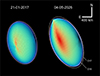 |
Fig. 4. Projections of the hydrostatic shape of configuration C in the sky plane at the time of the 2017 occultation (left) and the future 2026 occultation (right). The projected ellipses obtained by Ortiz et al. (2017) and the projection of the ellipsoids from Ortiz et al. (2017, O17) and Dunham et al. (2019, D19) are shown in the left and right panels, respectively, as dotted white lines for comparison. The facet colours code the relative irradiance they receive, red being the highest and bluish purple the lowest. |
Acknowledgments
We are grateful to B. Sicardy for fruitful discussions about the occultations of 2017 and 2026 and to S. Charnoz for informed comments on the manuscript before submission. We thank the referee, S. Desch, for pointing out the problem with the rotational phase in Ortiz et al. (2017). This work has been supported by the French Agence Nationale de la Recherche, project Roche, number ANR-23-CE49-0012.
References
- Barnouin, O., Ballouz, R.-L., Marchi, S., et al. 2024, Nat. Commun., 15, 6202 [Google Scholar]
- Barr, A. C., & Schwamb, M. E. 2016, MNRAS, 460, 1542 [NASA ADS] [CrossRef] [Google Scholar]
- Brozović, M., & Jacobson, R. A. 2024, AJ, 167, 256 [Google Scholar]
- Castillo-Rogez, J., Weiss, B., Beddingfield, C., et al. 2023, J. Geophys. Res.: Planets, 128, e2022JE007432 [Google Scholar]
- Desch, S. J., Cook, J. C., Doggett, T. C., & Porter, S. B. 2009, Icarus, 202, 694 [NASA ADS] [CrossRef] [Google Scholar]
- Drummond, J. D., Cocke, W. J., Hege, E. K., & Strittmatter, P. A. 1985, Icarus, 61, 132 [NASA ADS] [CrossRef] [Google Scholar]
- Dunham, E. T., Desch, S. J., & Probst, L. 2019, ApJ, 877, 41 [NASA ADS] [CrossRef] [Google Scholar]
- Holler, B. J., Grundy, W. M., Buie, M. W., & Noll, K. S. 2021, Icarus, 355, 114130 [NASA ADS] [CrossRef] [Google Scholar]
- Jorda, L., Lamy, P. L., Gaskell, R. W., et al. 2012, Icarus, 221, 1089 [NASA ADS] [CrossRef] [Google Scholar]
- Kondratyev, B. P., & Kornoukhov, V. S. 2018, MNRAS, 478, 3159 [Google Scholar]
- Lacerda, P., Jewitt, D., & Peixinho, N. 2008, AJ, 135, 1749 [CrossRef] [Google Scholar]
- Lanzano, P. 1982, Deformations of an Elastic Earth (New York: Academic Press) [Google Scholar]
- Lockwood, A. C., Brown, M. E., & Stansberry, J. 2014, Earth Moon Planets, 111, 127 [NASA ADS] [CrossRef] [Google Scholar]
- Maeder, A., & Meynet, G. 2012, Rev. Mod. Phys., 84, 25 [Google Scholar]
- McKinnon, W. B., Glein, C. R., Bertrand, T., & Rhoden, A. R. 2020, The Pluto System After New Horizons (Tucson: University of Arizona Press), 507 [Google Scholar]
- Murray, C. D., & Dermott, S. F. 1999, Solar System Dynamics (Cambridge: Cambridge University Press) [Google Scholar]
- Noviello, J. L., Desch, S. J., Neveu, M., Proudfoot, B. C. N., & Sonnett, S. 2022, Planet. Sci. J., 3, 225 [Google Scholar]
- Ortiz, J. L., Thirouin, A., Campo Bagatin, A., et al. 2012, MNRAS, 419, 2315 [NASA ADS] [CrossRef] [Google Scholar]
- Ortiz, J. L., Santos-Sanz, P., Sicardy, B., et al. 2017, Nature, 550, 219 [NASA ADS] [CrossRef] [Google Scholar]
- Ortiz, J. L., Morales, N., Ocaña-Pastor, A., et al. 2026, MNRAS, 548, stag692 [Google Scholar]
- Proudfoot, B. C. N., Ragozzine, D. A., Giforos, W., et al. 2024, Planet. Sci. J., 5, 69 [Google Scholar]
- Rizos, J. L., Ortiz, J. L., Gutierrez, P. J., Navajas, I. M., & Lara, L. M. 2025, A&A, 703, A178 [NASA ADS] [CrossRef] [EDP Sciences] [Google Scholar]
- Staelen, C., & Huré, J.-M. 2026, A&A, 708, A316 [NASA ADS] [CrossRef] [EDP Sciences] [Google Scholar]
- Zharkov, V. N., & Trubitsyn, V. P. 1978, Physics of Planetary Interiors (Tucson: Pachart Publishing House) [Google Scholar]
Appendix A: Light curves
The Hapke model was used for the reflectance of Haumea, with the same parameters as Lockwood et al. (2014) and a darker spot covering a quarter of Haumea with a 10% albedo variation (Lacerda et al. 2008). We reproduce three light curves reported in Lacerda et al. (2008), Lockwood et al. (2014) and Ortiz et al. (2017); the results are shown in Fig. A.1. Note that only the light curve obtained with configuration C is plotted in Fig. A.1, but the curves obtained with the other configurations are actually similar to the one reported here. The pinched shape leaves a mark in the light curve, with slightly narrower maxima and slightly larger minima. However, this feature would be difficult to detect on real light curves due to the limited resolution or albedo variations on the surface. Thus, it appears that only stellar occultation could allow us to observe if Haumea has an ellipsoidal or a pinched shape.
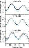 |
Fig. A.1. Comparisons between the light curves of Haumea reported by Lacerda et al. (2008, top), Lockwood et al. (2014, middle), and Ortiz et al. (2017, bottom) and synthetic light curves obtained with the hydrostatic figures. |
All Tables
Examples of hydrostatic solutions whose free surface is coherent with the chords obtained during the 2017 occultation (Ortiz et al. 2017).
All Figures
|
Fig. 1. Possible hydrostatic models obtained in this work (pink region). The models listed in Table 1 are plotted with black crosses. For reference, the Jacobi sequence is plotted as a red line. The best-fit ellipsoids from Ortiz et al. (2017, ‘O17’) and the hydrostatic model preferred by Dunham et al. (2019, ‘D19’) are reported with open circles. The ‘shadow ellipsoids’ curve corresponds to ellipsoids whose projection corresponds to the ellipse determined during the 2017 occultation, with the pole orientation obtained by Ortiz et al. (2017) and a rotational phase of −13.3°; see Drummond et al. (1985) for the equations used. Note that this curve is valid only for ellipsoidal shapes. |
| In the text | |
|
Fig. 2. Hydrostatic shape models for Haumea in the (xOz) (left) and (yOz) (right) planes, corresponding to the configurations reported in Table 1. The dashed lines correspond to the ellipsoids with the same axis lengths as the layers’ boundary. |
| In the text | |
|
Fig. 3. Projections of the six hydrostatic representative solutions in the sky plane at the epoch of the 2017 occultation. u and v are celestial east and north, respectively. The pole orientation is the one obtained by Ortiz et al. (2017), and the rotational phase is −13.3°. |
| In the text | |
|
Fig. 4. Projections of the hydrostatic shape of configuration C in the sky plane at the time of the 2017 occultation (left) and the future 2026 occultation (right). The projected ellipses obtained by Ortiz et al. (2017) and the projection of the ellipsoids from Ortiz et al. (2017, O17) and Dunham et al. (2019, D19) are shown in the left and right panels, respectively, as dotted white lines for comparison. The facet colours code the relative irradiance they receive, red being the highest and bluish purple the lowest. |
| In the text | |
|
Fig. A.1. Comparisons between the light curves of Haumea reported by Lacerda et al. (2008, top), Lockwood et al. (2014, middle), and Ortiz et al. (2017, bottom) and synthetic light curves obtained with the hydrostatic figures. |
| In the text | |
Current usage metrics show cumulative count of Article Views (full-text article views including HTML views, PDF and ePub downloads, according to the available data) and Abstracts Views on Vision4Press platform.
Data correspond to usage on the plateform after 2015. The current usage metrics is available 48-96 hours after online publication and is updated daily on week days.
Initial download of the metrics may take a while.