


| Issue |
A&A
Volume 710, June 2026
|
|
|---|---|---|
| Article Number | A212 | |
| Number of page(s) | 24 | |
| Section | The Sun and the Heliosphere | |
| DOI | https://doi.org/10.1051/0004-6361/202659355 | |
| Published online | 19 June 2026 | |
Constraints and observational manifestations of failed solar eruptions in a toroidal magnetic cage
1
School of Astronomy and Space Science and Key Laboratory of Modern Astronomy and Astrophysics, Nanjing University, Nanjing 210023, China
2
Centre for Mathematical Plasma Astrophysics, Department of Mathematics, KU Leuven, Celestijnenlaan 200B, B-3001 Leuven, Belgium
3
LIRA, Observatoire de Paris, CNRS, UPMC, Université Paris Diderot, 5 place Jules Janssen, 92190 Meudon, France
4
LUNEX EMMESI Institut, SBIC, Kapteyn straat 1, Noordwijk2201 BB, The Netherlands
5
Institute of Physics, University of Maria Curie-Skłodowska, ul. Radziszewskiego 10, 20-031 Lublin, Poland
6
State Key Laboratory of Solar Activity and Space Weather, National Space Science Center, Chinese Academy of Sciences, Beijing, 100190, China
7
CAS Key Laboratory of Geospace Environment, Department of Geophysics and Planetary Sciences, University of Science and Technology of China, 230026 Hefei, China
★ Corresponding author: This email address is being protected from spambots. You need JavaScript enabled to view it.
Received:
6
February
2026
Accepted:
23
March
2026
Abstract
Context. Observations show that many solar eruptions remain confined in the magnetic configuration of strong overlying magnetic fields, which is commonly referred to as the magnetic cage.
Aims. Confined eruptions under strong, poloidal overlying fields have been widely studied. In contrast, the confined eruption scenario under strong external toroidal fields remains unknown.
Methods. We used three-dimensional magnetohydrodynamic simulations to systematically study confined eruptions in a toroidal magnetic cage, focusing on the roles of the Lorentz force and magnetic reconnection, as well as their observational manifestations, such as flare ribbons and loops. We further applied the test-particle method with the guiding-centre approximation to synthesize hard X-ray sources, enabling comparison between thermal and nonthermal responses.
Results. Our results show that overlying toroidal magnetic fields are crucial in confining eruptions. They generate strong return currents that produce a significant downward Lorentz force, suppressing the rise of the flux rope. Simultaneously, they drive the large-angle rotation of the rope, triggering reconnection with the overlying fields and ultimately causing its breakup. The synthesized EUV images display multi-ribbon flare structures with highly sheared loops with a global “cowboy-hat-like” shape. Additionally, comparisons with hard X-ray sources reveal that thermal and nonthermal responses are not co-spatial, in which return current is a major accelerator to energetic electrons.
Conclusions. The simulations clarify how the magnetic cage constrains solar eruptions. First, the downward Lorentz force related to return current effectively suppresses eruptions, explaining why confined flares tend to occur in electric-current neutralized active regions. Second, we demonstrate that toroidal-field-induced force is the key driver for rotation and confinement of the flux rope. This explains why many filament eruptions with rotation fail despite being torus-unstable. Finally, we suggest that the global morphology of flare loops (cowboy-hat–like or “saddle-like”) and the shearing degree of flare loops can serve as useful diagnostics to distinguish confined from eruptive flares.
Key words: magnetohydrodynamics (MHD) / methods: numerical / Sun: corona / Sun: flares / Sun: magnetic fields
© The Authors 2026
 Open Access article, published by EDP Sciences, under the terms of the Creative Commons Attribution License (https://creativecommons.org/licenses/by/4.0), which permits unrestricted use, distribution, and reproduction in any medium, provided the original work is properly cited.
This article is published in open access under the Subscribe to Open model. This email address is being protected from spambots. You need JavaScript enabled to view it. to support open access publication.
1. Introduction
Solar eruptions, such as solar flares and coronal mass ejections (CMEs), are widely recognized as the most intense activities in the Solar System (Chen 2011). Research in this field is constantly a priority in both astrophysics and solar–terrestrial space physics. On the one hand, the extensively observed solar eruptions encompass numerous fundamental astrophysical processes (Tsurutani et al. 2023). This suggests that novel insights into the explanation of other high-energy astrophysical phenomena may be obtained by analogy with solar eruptions (Dai et al. 2006; Meng et al. 2014). On the other hand, solar eruptions can expel a substantial amount of magnetized plasma into interplanetary space, thereby giving rise to disturbances in the solar–terrestrial space environment. As a result, exploring the dominant underlying physical mechanisms of solar eruptions is of great importance both for forecasting adverse space-weather events and enhancing our understanding of the Universe.
Although almost all solar eruptions can release substantial electromagnetic radiation–namely solar flares–not all solar eruptions can produce CMEs. If the eruptive core manages to break through the constraints of the overlying fields and escapes into interplanetary space, it will evolve into a CME and later on into an interplanetary CME (ICME). These successful solar eruptions, or eruptive flares, have the potential to induce geomagnetic storms and thus jeopardise human satellite operations. However, in certain events, eruptive cores fail to escape from the solar corona (Ji et al. 2003; Nindos et al. 2015; Thalmann et al. 2015; Zuccarello et al. 2017). They are often referred to as confined flares or failed eruptions. Exactly how to predict eruptive and confined flares is still a crucial and challenging aspect of space-weather research.
Previous studies have shown that the success or confinement of solar eruptions is strongly influenced by their magnetic environment, particularly the eruptive core and the overlying background fields. For instance, Wang & Zhang (2007) reported that confined flares preferentially occur near the center of active regions, highlighting the role of overlying fields in producing confinement. Similarly, Li et al. (2021) implied that magnetic flux is a decisive quantity to distinguish eruptive and confined flares. Further studies revealed that eruptions are more likely to fail if the critical height (e.g., where the decay index n(r) = 1.5) is high (Wang et al. 2017; Li et al. 2022) or if the n(r) profile exhibits a saddle-like profile with a dip (Guo et al. 2010), in which the decay index first rises, then dips, and finally increases again with height (see Figure 2 for the decay index derived from the total horizontal field). From laboratory plasma experiments, Myers et al. (2015) proposed a combined parameter of the decay index (n) and the safety factor (1/Tw) to better differentiate confined and eruptive flares, a criterion later tested in solar plasma environments by Jing et al. (2018) and Duan et al. (2019). Li et al. (2022) proposed a new parameter considering the force-free factor (α) of core fields and magnetic flux to distinguish two types of flares. Recently, Teraoka et al. (2025) demonstrated that the amount of twist and the height of field lines connecting flare kernels can distinguish eruptive from confined flares.
Although these statistical findings reveal key discriminants between confined and eruptive flares, the underlying physical mechanisms remain poorly understood. For example, numerous failed filament eruptions are torus-unstable (n > 1.5) and exhibit large-angle rotation (Ji et al. 2003; Zhou et al. 2019; Guo et al. 2024). Additionally, counterexamples in Jing et al. (2018) and Duan et al. (2019) may reflect the possibility that external magnetic reconnection sometimes plays a negative role in forming CMEs. In this scenario, the toroidal-field-induced tension force (Myers et al. 2015; Zhang et al. 2024; Guo et al. 2024), non-axisymmetry-induced force (Zhong et al. 2021), and external magnetic reconnection involving the flux rope (Jiang et al. 2023; Chen et al. 2023) may have some effects resulting in failed eruptions. Recently, Liu et al. (2017) and Liu et al. (2024) pointed out that the amount of non-neutralized electric current, measured by the ratio of photospheric direct current (DC) to return current (RC), is a reliable proxy for assessing the success or not of an eruption. Direct current (DC) is generally associated with the twist of a flux rope and is often concentrated near the core of the flux tube. The return current forms a surrounding surface current that envelopes the DC, effectively isolating the flux tube from its ambient magnetic environment. However, why active regions with neutralised electric current prefer to form confined flares remains a subject of debate.
To better distinguish between confined and eruptive flares, it is essential to establish a basic framework for different magnetic configurations. Existing numerical MHD models of confined flares have largely focused on cases with strong overlying poloidal fields (Török & Kliem 2005; Jiang et al. 2023) or on magnetic configurations involving a null point where the flux from outer polarities exceeds that of the core fields (Chen et al. 2023). However, the scenario of strong overlying toroidal fields (the so-called toroidal magnetic cage) remains less explored because the eruptive flux rope easily escapes from the overlying toroidal magnetic fields intuitively, as shown in Fan & Gibson (2007). Actually, the downward force induced by the toroidal field scales with the square of the electric current intensity, whereas the downward force induced by the poloidal field scales linearly with the current. This implies that toroidal fields can also play a significant role in suppressing the eruption. In addition, the toroidal field can drive a large-angle rotation of the flux rope (Kliem et al. 2012; Zhou et al. 2023; Zhang et al. 2024; Guo et al. 2024), which alters the distribution of the resulting Lorentz force and may also generate an external Lorentz force. These indicate that the role of overlying toroidal fields cannot be neglected.
To this end, we carried out a series of MHD simulations and conducted a systematic analysis encompassing (1) the evolution of magnetic fields, (2) electric currents, (3) Lorentz force, (4) magnetic reconnection, and (5) forward modelings (thermal and nonthermal). The organization of this paper is as follows. Section 2 introduces the numerical setup, and Section 3 presents the global evolution of simulation results. Subsequent sections analyze the confined mechanisms (Section 4) and forward-modeling results (Section 5). We conclude with the discussion and summary in Sections 6 and 7.
2. Numerical setup
2.1. Magnetic configuration
We built the initial magnetic configuration similarly to the one introduced in Titov & Démoulin (1999) and Titov et al. (2014). The external poloidal field (Bp) is defined by two sub-photosphere magnetic charges of qP strength positioned along the x-axis at a depth of dP and separated by 2LP. Next, to introduce toroidal fields (BT) aligned with the flux-rope axis (y-axis), two additional magnetic charges of qT strength were placed on the y-axis at y = ±LT with a depth of qT. Bp, BT, and their combinations are in accordance with the potential field model without electric currents. The core fields were then constructed by embedding a force-free toroidal flux rope (BFR) along the y-axis. BFR is characterized by its major radius, R, and its minor radius, a. It is implemented with the regularized Biot-Savart laws (Titov et al. 2018). The equilibrium current in the flux rope is governed by Shafranov’s stability criterion (Equation 7 in Titov et al. 2014). We call the above model FR-PT, while it is denoted FR-P when only the external poloidal fields are included.
To better reach a force-free state in the initial magnetic configuration, we employed a magneto-frictional relaxation on the superimposed fields (Guo et al. 2016). Figure 1 displays the magnetic configuration with the following parameters: R = 30 Mm, a = 12 Mm, qP = 150 T Mm2, qT = 600 T Mm2, dP = 10 Mm, dT = 50 Mm, LP = 10 Mm, and LT = 100 Mm. In this figure, we can see a twisted flux rope (yellow lines), overlying poloidal field lines connecting PP and NP polarities (cyan lines), and overlying large-scale toroidal field lines connecting PT and NT polarities (pink lines).
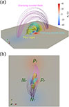 |
Fig. 1. Visualization of the initial magnetic fields viewed from the (a) side and (b) top. The yellow, cyan, and magenta tubes represent the twisted flux rope and the overlying poloidal and toroidal magnetic fields, respectively. NP/NT and PP/PT label the negative and positive sub-photosphere magnetic charges to build the poloidal/toroidal magnetic fields, respectively. |
Figure 2 shows the profiles of the decay index: np (orange line), nt (green line), and nh (blue line). They are computed from Bp, BT, and Bh = BT + Bp components, respectively, with the following formula:
 (1)
(1)
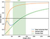 |
Fig. 2. Height profiles of decay index computed from external total horizontal magnetic fields (Bh, blue line), poloidal fields (Bp, orange line), and toroidal fields (BT, green line). The orange and green bands indicate regions of the flux rope at initial and stopping moments, respectively. The associated movie is available online. |
where Bex is the selected horizontal magnetic-field component. The decay index, nh, calculated from Bh exhibits a saddle-like profile, while the profiles of nt and np monotonically increase. The flux rope is positioned near the typical threshold (np = 1.5) of torus instability (Aulanier et al. 2010), enabling the triggering of an eruption despite the initial equilibrium. It should be noted that the flux-rope-occupied areas (red and green bands) are determined by the Lorentz force (JFR × BT) in Figure 9d.
2.2. Magnetohydrodynamic modeling
We employed a thermodynamic MHD model considering the thermal conduction to simulate the eruption process. The governing equations are as follows:
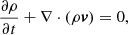 (2)
(2)
![Mathematical equation: $$ \begin{aligned}&\frac{\partial (\rho \boldsymbol{v})}{\partial t} + \nabla \cdot \left[\rho \boldsymbol{v}\boldsymbol{v} + \left(p+\frac{\boldsymbol{B}^{2}}{2\mu _{0}}\right)\boldsymbol{I} - \frac{\boldsymbol{BB}}{\mu _0}\right] = \rho \boldsymbol{g},\end{aligned} $$](/articles/aa/full_html/2026/06/aa59355-26/aa59355-26-eq3.gif) (3)
(3)
 (4)
(4)
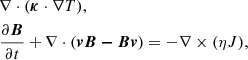 (5)
(5)
where  is field-aligned thermal conduction,
  is the Spitzer heat conductivity, g = −k g⊙ r⊙2/(r⊙ + z)2ez represents the gravitational acceleration, g⊙ = 274 m s−2 is the gravitational acceleration at the solar surface, r⊙ is the solar radius, η = 4.65 × 1011 cm2 s−1 is the uniform resistivity, and other variables have their general meanings. The imposed resistivity, η, is comparable to that used by Kilpua et al. (2021) and has two main effects. First, it improves numerical stability when a high-order limiter is employed. Second, it accounts for Joule heating in regions of strong electric current. Following Jiang et al. (2021b), we scaled gravitational acceleration by a factor of k = 1.8. This operation can effectively reduce the scale height, and it ensures that plasma β < 1 even in the overlying weak magnetic fields. The environment of β < 1 throughout the computational domain ensures that the eruption dynamics are dominated by magnetic fields in solar active regions rather than thermodynamic effects. The plasma density is initialized using an isothermal hydrostatic atmospheric model with uniform temperature (1 MK).
The three-dimensional (3D) MHD equations are numerically solved with the Message Passing Interface Adaptive Mesh Refinement Versatile Advection Code (MPI-AMRVAC, Xia et al. 2018; Keppens et al. 2023). We used Cartesian coordinates, with a domain of [xmin,xmax] × [ymin,ymax] × [zmin,zmax] = [−150, 150] × [−150,150] ×[0,300] Mm3. We used a four-level adaptive mesh refinement with a basic mesh grid of 40 × 40 × 40 points. To mitigate the divergence of the magnetic fields during the numerical calculation, we employed the constrained-transport (CT) method on staggered grids (Gardiner & Stone 2005). This method keeps the divergence of magnetic fields unchanged up to machine accuracy. This can be evaluated by the < |fi|> = (∑i|fi|ΔVi)/(∑iΔVi > ) ∼ 10−16, where fi = (∇⋅B)iΔVi/BiAi denotes the fractional flux increase in a small discrete volume about grid point i, Vi, Ai, and Bi represent the cell volume, cell surface area, and the magnitude of the magnetic field at point i, respectively. The validity of this approach is discussed in Schmieder et al. (2024).
Regarding the numerical scheme, we adopted an HLL flux scheme, a three-step Runge–Kutta time discretisation approach, and the fifth-order WENO-limited reconstruction. For the bottom boundary conditions, we implemented a line-tied condition as follows. First, we set the horizontal electric field (Eh) on the lower bottom plane to zero, ensuring that the normal magnetic-field component remains unchanged over time. Second, the plasma velocities were set to zero in the bottom plane between the inner ghost cells and the physical domains. The lateral and top boundaries are prescribed as open with zero-gradient extrapolation.
3. Global evolution during eruption
Figure 3 illustrates the 3D dynamic evolution of magnetic fields during the eruption. The flux rope erupts directly due to torus instability. As it rises, a current sheet forms beneath it, where magnetic reconnection generates highly sheared loops. Meanwhile, the pre-existing flux rope (yellow lines) undergoes a clockwise rotation, reaching 90° by about t = 6τ (τ = 85.87 s is the normalisation unit in the simulation). This rotation direction is consistent with observations showing that sinistral filaments (positive helicity) tend to rotate clockwise (Green et al. 2007). It should be noted that the asymmetry in the simulation results may be associated with the nonlinear WENO5 reconstruction and the rotation of the flux rope. As the underlying magnetic reconnection persists, the flux rope undergoes a gradual, decelerating rise. Eventually, the structure reverses its motion and begins to descend, with the newly reconnected field lines anchored to the northern toroidal polarity (NT). This implies the reconnection between the eruptive flux rope and the overlying toroidal fields.
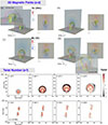 |
Fig. 3. Temporal evolution of (a–d) magnetic-field and (e, f) twist-number Tw distributions in the eruption process. The yellow, cyan, and pink tubes are traced from the NFR, NP, and NT polarities, respectively. The colors in the bottom and vertical planes exhibit the distributions of the Bz and Te, respectively. Panels (e) and (f) display the Tw distributions on the vertical and bottom planes, respectively. |
To further elucidate the topology evolution during the eruption, we computed the twist-number (Tw) distributions using the parallel electric-current (J∥ = J ⋅ B/B) integration method (Berger & Prior 2006; Liu et al. 2016) as follows:
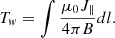 (6)
(6)
Figures 3e and 3f show the distribution of Tw distribution on the side and bottom planes, respectively. The initial extension of the flux-rope footpoints, accompanied by an increase in Tw, reflects magnetic reconnection in the ambient arcades (Figure 3c). Subsequently, Tw decreases as the twist is partially converted into writhe (manifested as the rotation of the flux rope) and further reduced by reconnection between the flux rope and the overlying toroidal fields. Notably, a shell of opposite-sign twist develops around the flux rope, corresponding to return current (RC).
Figure 4 shows the temporal evolution of the toroidal magnetic field (By), number density (n), and temperature (Te) in the x–z plane. Similarly to the twist distribution in Figure 3e, the outer shell of the eruptive core exhibits a +By component opposite to that of the central region, where the plasma is heated to twice the background temperature. In contrast, the temperature and density inside the circular dome decrease due to expansion. The reversal of the By component is due to the flux rope’s rotation, with the rotation angle increasing with height, as shown in Figure 3. Consequently, regions with positive, zero, and negative By correspond to rotation angles greater than, equal to, and less than 90°, respectively. This is also validated in Figure 10d, corresponding to strong −Bx component and positive By component. In addition, the heated current sheet beneath the flux rope is consistent with the standard flare model. A heated and dense plasma blob also appears in the upper-right portion of the flux rope at t = 15τ, suggesting external magnetic reconnection involving the flux rope. To further quantify the flux rope kinematics, we measured the height of the outer +By shell to derive its velocity. As shown in Figure 5, the flux rope accelerates to 150 km s−1 at t = 3τ and then decelerates to –10 km s−1 at t = 12τ, indicating a failed eruption.
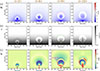 |
Fig. 4. Temporal evolution of (a) the axial magnetic field component, By; (b) the number density, n; and (c) the temperature, Te, at t = 2, 6, 9, 15τ. The dashed line in the t = 9 column outlines the border of the flux rope (with added reconnected flux). |
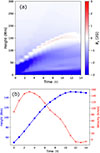 |
Fig. 5. Kinematics of eruptive flux rope. Panel (a) shows the time–distance diagram of the By component along the z-axis. In panel (b) the blue dots and red crosses show the evolution of height and velocity during the eruption, which are measured with the positive By front in panel (a). |
The temperature distribution on the bottom plane, shown in Figures 6(a1)–(a6), reflects the evolution of flare ribbons to a great extent. As seen in the top panels, the heated regions form elongated two-ribbon structures, closely resembling the separated flare ribbons in observations. Away from the central portion, the ribbons show hook-like shapes, corresponding to the footpoints of the flux rope. Initially, the ribbons extend along the PIL and subsequently separate perpendicular to it, which is consistent with the 3D standard-flare model (Janvier et al. 2014). After t = 10τ, two additional heated spots appear at the ribbon endpoints, as shown in Figure 6(a6). To further analyze the magnetic topology, we computed the distribution of the squashing degree Q (Priest & Démoulin 1995; Démoulin et al. 1996a), shown in Figures 6(b1)–(b6). Quasi-separatrix layers (QSLs) are areas where magnetic connectivity changes drastically, and the squashing factor (Q) is larger than 2. They are favorite locations for magnetic reconnection (Priest & Démoulin 1995; Démoulin et al. 1996a; Titov et al. 2002). The closed circular QSLs outline the footpoints of the twisted flux rope, while the separated straight QSLs correspond to two flare ribbons. During the eruption, the circular QSLs drift along the y-axis, expand significantly, and eventually merge with the outer hooked QSLs, as predicted by Chen et al. (2012). Fine structures at the hook endpoints are also evident, coinciding with the additional heated regions in Figure 4b and the outer twist shell with opposite helicity (Figure 3f). To quantify the ribbon dynamics, we extracted a slit along the separation direction of the ribbons in Figure 6(a3). The time–distance diagrams of temperature (Te) and QSLs, shown in Figures 6(c) and 6(d), reveal nearly identical behaviors: the ribbons initially separate at ∼30 km s−1, gradually decelerate, and eventually stop near x = ±30 Mm. This demonstrates that confined flares can also exhibit ribbon-separation motions.
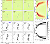 |
Fig. 6. Evolution of flare ribbons depicted from the (a, c) temperature and (b, d) QSL distributions. Temporal evolution of the (a) temperature and (b) squashing degree, Q, of QSLs on the bottom plane. Panels (c) and (d) show the time–distance diagram of temperature and Q along the blue line in Panel (a3), respectively. Two wave-like fronts in Panels (a3) and (a4) correspond to the shock in Figure 4c. The artifacts of Q near the side boundaries arise from the finite size of the computational domain. However, they do not give rise to significant heating fronts, electric currents, or Lorentz forces, and thus they have only a small impact on the derived conclusions. The box size is equal to that in plots (e) and (f) of Figure 3. |
Figure 7 shows the distribution of electric current. Panels in rows (a)–(c) display the Jx, Jy, and Jz components in the x − z plane, respectively. An outer electric current shell with an opposite sign relative to the central core is evident, corresponding to the RC. The RC regions are nearly co-spatial with the outer shells of negative twist (Tw), as expected from the definition of Tw (Figures 3e and 3f). Regarding the evolution, the return current is initially much weaker than the direct current flowing through the flux rope, but it becomes comparable by the final stage of the eruption as the direct current rapidly decreases. Figure 7d presents the normal electric current (Jz) on the bottom plane. The modeled active region is strongly non-neutralized due to the pre-existing flux rope, with an initial |DC/RC| ratio of 8.9 (Figure 8a). The DC (RC) is computed from the integration of the positive/negative (negative/positive) current in positive/negative (negative/positive) magnetic-field polarity (∫JzdS). Three typical features characterize the electric current evolution: (1) return currents form around the hooked ends of flare ribbons, corresponding to twisted field lines of opposite current helicity (Figure 3f), but remain absent along the straight, separated ribbons (Janvier et al. 2014); (2) localized currents intensify along separated straight flare ribbons–consistently with results of Janvier et al. (2014)–due to the twist increase produced by magnetic reconnection, which converts sheared arcade fields into twisted flux-rope field lines, so as to increase the current density (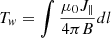 ); (3) the current density at the flux-rope footpoints decreases for two reasons. As shown in Figure 3, the pre-existing flux rope rotates during the eruption, which decreases the twist number through the conversion of twist into writhe, thereby reducing the current density. In addition, the stretching of magnetic-field lines can naturally reduce the twist density along a field line in ideal MHD conditions, which further lowers the current density.
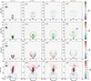 |
Fig. 7. Evolution of electric current during eruption. The first (a1–a4), second (b1–b4), and third (c1–c4) rows display the distributions of Jx, Jy, and Jz, respectively, in the central vertical plane. The (d1–d4) bottom row displays the distributions of Jz in the bottom horizontal plane. The dashed red (positive Bz) and black (negative Bz) lines represent the contour lines of Bz = ±40, 20, 10, and 5 G. In regions of positive/negative Bz (red/black contours), positive/negative currents (red/blue) represent the DC system, whereas negative/positive currents (blue/red) form the RC system. The 1D slits S1 and S2 are defined in panels (d3) and (d4) by yellow and pink segments, respectively, showing the. Some averaged quantities at z = 0 within these slits are shown in Figure 8. The associated movie is available online. |
Figure 8a shows the temporary evolution of |DC/RC|, which drops rapidly from 8.9 to 3.5 within 4 τ and then remains nearly constant thereafter. It is worth noting that, because our modeling is based on the TDm model incorporating a strong current-carrying flux rope, the resulting |DC/RC| ratio is larger than the typical values reported in observations (Liu et al. 2017). To further examine the magnetic properties of return current, we cut two slits along S1 (near poloidal polarity) and S2 (near toroidal polarity) in Figures 7(d3) and (d4), respectively. As illustrated in Figures 8b and 8c, the normal and horizontal magnetic fields at the direct-return current (DC–RC) transition points differ significantly between these two regions. For the return current near the poloidal polarities, the DC–RC transition point corresponds to the maximum horizontal magnetic fields (Bh) and minimum normal magnetic field (Bz), closely resembling the conditions at flux-rope footpoints in a simple bipolar magnetic configuration (Xing et al. 2024). However, for the RC near the toroidal polarity, the DC–RC transition point corresponds instead to the minimum horizontal field, Bh.
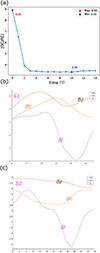 |
Fig. 8. Panel (a) shows the temporal evolution of |DC/RC| in the eruption process. Panels (b) and (c) display the average magnetic properties of the direct-return currents near the poloidal polarity (S1, Figure 7d3) and the toroidal polarity (S2, Figure 7d3). The violet, orange, and brown lines represent the profiles of normal electric current (Jz), horizontal magnetic field (Bh), and normal magnetic field (Bz), respectively. |
4. Confined mechanisms
As shown in Figure 5, our numerical model successfully reproduced a confined flare. Here, we investigate the mechanisms responsible for this confinement, with particular emphasis on the roles of the downward Lorentz force and magnetic reconnection.
4.1. Downward Lorentz force constraining the solar eruption
To investigate the origins and distributions of Lorentz force acting on the flux rope, we decomposed the total magnetic fields, B, in the simulation into external toroidal field (BT), external poloidal field (Bp), and flux-rope field (BFR):
 (7)
(7)
where BT and Bp are directly determined from the prescribed analytical solutions of toroidal (PT and NT) and poloidal (PP and NP) magnetic charges, respectively. The flux-rope component is then obtained as BFR = B − BT − Bp, enabling the calculation of the current density flowing through the flux rope via JFR = ∇ × BFR/μ0. It should be emphasized that because the magnetic field provided by the external poloidal and toroidal polarities satisfies the current-free potential field, the total electric current, J, is entirely attributable to the flux rope, namely J = JFR.
Figure 9 displays the vertical Lorentz force acting on the flux rope as it activates in the x − z plane. The temporal evolution of the net Lorentz force (Figure 9a) shows an initial upward-force dominance in the lower part of the flux rope, driving its acceleration before t = 3τ (Figure 4c). Subsequently, the downward Lorentz force becomes dominant, leading to a deceleration and eventual suppression of the eruption, with the flux rope reaching a downward velocity of −10 km s−1 at t = 12τ.
 |
Fig. 9. Distribution of vertical Lorentz force in the x − z plane at the times of 2, 6, 9, and 15 τ. Panels (a)–(d) exhibit the vertical component of Lorentz force induced from total magnetic fields, flux-rope fields, external poloidal fields, and toroidal fields, respectively. |
To quantify the contributions from different magnetic components, we computed Lorentz force arising from the interaction of the current flowing through the flux rope (JFR) with (1) the flux rope itself (BFR, Figure 9b), (2) the external poloidal fields (Bp, Figure 9c), and (3) the external toroidal fields (BT, Figure 9d). These are hereafter referred to as the self-force, Bp-induced force, and BT-induced force, respectively. Following the terminology of Myers et al. (2015, 2016), these correspond to the classical hoop force, strapping force, and tension force1. In the following, we use this decomposition to assess how different magnetic-field components govern the dynamics of the flux-rope eruption.
Figure 9a shows the distribution of the net Lorentz force, where the dominant downward Lorentz force arises mainly from the flux-rope core and its surrounding shell. Below, we investigate the origins of this downward component. Figure 9b illustrates the self-force of the flux rope. A comparison with the net Lorentz force distribution indicates that the net downward Lorentz force in the flux-rope (panel a) is not due to this self-force. Figure 9c demonstrates that the poloidal field-induced Lorentz force initially provides a downward strapping effect, covering the entire flux rope. However, as the flux rope rises, this restraining contribution weakens, approximately balancing the upward gradient of magnetic pressure. The expansion of the flux rope during the eruption further reduces JFR, while the simultaneous decrease in Bp diminishes the strapping effect, as reflected in the net Lorentz-force distribution after t > 8τ.
The toroidal field-induced Lorentz force, however, exhibits different behavior. First, it acts in opposite directions on the upper and lower portions of the flux rope because the azimuthal current (Figure 7a) interacts with the unit-directional BT field (Figure 9d). As a result, the distribution of the toroidal field-induced Lorentz force can be used to determine the occupied areas of the flux rope. Second, a concentric outer shell of negative-sign current develops around the leading part of the eruptive dome, generating strong downward forces as early as t = 3τ and persisting thereafter. Because the flux rope is embedded in a strongly sheared, BT-dominated magnetic environment (Figure 3 a), the magnitude of the BT-induced force exceeds that of the Bp-induced force by roughly an order of magnitude. Consequently, the net Lorentz force globally remains directed downward (Figure 9a), highlighting the toroidal field as the primary factor constraining the eruption. This conclusion is further supported by the decay index profiles derived from the different magnetic-field components (Figure 2), which show that the toroidal field decreases more slowly with height than the poloidal field.
Figure 10 illustrates the spatial relationships among the magnetic topology, electric-current systems (such as DC and RC), and Lorentz force. Figures 10a and 10b display the field lines rooted in regions of direct currents (yellow, green, purple, and pink lines) and RCs (cyan and red lines), respectively. Figure 10c presents the distribution of the vertical Lorentz force in the x − z plane. It is found that the return current near the toroidal polarity (magenta lines) produces a downward Lorentz force, whereas the return current near the poloidal polarity (cyan lines) produces an upward Lorentz force. To further explore the origin of the downward Lorentz force, Figure 10d shows the distributions of Jx, Jy, Bx, and By. The magenta and cyan field lines have the same Jx, but they differ in Jy in the direction due to rotation. In terms of magnetic fields, both exhibit negative Bx components but differ in By. Consequently, the Lorentz force acting on the magenta and cyan field lines points downward and upward, respectively. In summary, these results suggest that the return currents near toroidal polarities are crucial in confining solar eruptions.
 |
Fig. 10. Relationship among magnetic-field lines and the electric current, Lorentz force, and magnetic-field components. Panels (a) and (b) show the field lines traced from DC (yellow, green, cyan, and blue lines) and RC (red and magenta lines). Panel (c) shows the distribution of the vertical Lorentz force on the X-Z plane. Panel (d) displays the distribution of Jx, Jy, Bx, and By on the x-z plane. |
To further investigate the role of toroidal fields, we conducted a control group of an eruption without toroidal polarities, as described in Appendix A.1. As shown in Figure A.1, the control case demonstrates that a successful eruption occurs when only external poloidal fields are included (model FR-P), which suggests the critical role of external toroidal fields in producing failed eruptions. In the successful eruption case, flare ribbons exhibit the typical two-ribbon morphology and are associated with a higher degree of non-neutralized electric current compared to the confined eruption case.
4.2. Lateral Lorentz force driving the flux-rope rotation
As illustrated in Figure 3b, the flux rope rotates clockwise during its eruption, thereby changing the distribution of the Lorentz force acting upon the flux rope. Consistent with the observations, we define a clockwise rotation as the rotation seen when viewing from above (top-down). Notably, the rotation angle in the successful eruption (model FR-P, Figure A.1) is relatively smaller than in the confined eruption (model FR-PT). Hence, understanding the factors driving flux-rope rotation is important for the dynamics of the flux rope.
To this end, similarly what we did when analyzing the downward Lorentz force (Figure 9), we decomposed the lateral Lorentz force in the x − y plane at a height of approximately 50 Mm into contributions from the flux-rope self-force itself (JFR × BFR), the external poloidal-field-induced (JFR × Bp) and toroidal-field-induced Lorentz forces (JFR × BT). The flux-rope rotation is primarily induced by the component orthogonal to the flux rope, that is, mainly the x-component. All Lorentz-force components have opposite signs in the two flux rope legs; this induces a torque that rotates the flux rope’s upper part (as its footpoints are line-tied).
As shown in Figure 11, the main forces are concentrated within the flux rope, with weaker forces of opposing directions located at the flux-rope boundaries within the return current region. The Lorentz force arising from the external poloidal fields is significantly smaller than the other two contributions. In contrast, the Lorentz forces from the flux rope itself and the external toroidal fields act in opposite directions, producing counterclockwise and clockwise rotations, respectively. This implies that the external toroidal field dominates and determines the rotation direction of the flux rope. Consequently, the rotation does not necessarily reflect intrinsic magnetic properties of the flux rope, such as its twist, suggesting that rotation is not a reliable indicator of kink instability when the flux rope is embedded in strong external toroidal or sheared fields.
 |
Fig. 11. Distribution of lateral Lorentz force in the x-z plane at the times of 2, 6, 9, and 15 τ. Panels (a)–(c) exhibit the horizontal x component of Lorentz force induced from the flux rope itself, external poloidal fields and toroidal fields, respectively. The plane is selected at z = 50 Mm, as shown in Figure 9a. The inserted image in Panel (a) at t = 9 shows the Jz distribution and the corresponding field lines. |
To further assess the role of flux rope self-force itself, we removed both the poloidal and toroidal polarities and simulated the eruption of an isolated flux rope (Figure B.1). This setup excludes other influences on the flux rope dynamics, such as magnetic reconnection at the leading edge and Lorentz forces from external fields. We find that the flux rope largely maintains a toroidal shape and exhibits only weak rotation during the eruption, indicating that its self-force is not the dominant factor controlling rotation.
In summary, the Lorentz-force analysis suggests that strong external toroidal fields can induce a return current at the leading front of the flux rope. This generates a substantial downward Lorentz force that suppresses the rise of the flux rope. Moreover, the external toroidal field itself plays the dominant role in driving flux-rope rotation. This explains why so many failed eruptions are frequently accompanied by filament rotation (Zhou et al. 2019).
4.3. External magnetic reconnection destroying the flux rope
A natural consequence of flux-rope rotation is the formation of thinner QSLs in the interface between the flux rope and overlying field lines. This generates intense electric currents, which in turn drive magnetic reconnection involving the eruptive flux rope and finally destroys it. To examine the role of magnetic reconnection in modifying the flux-rope field lines, we traced two representative field lines located near the QSLs and followed their evolution in the eruption process.
Figures 12a–12d illustrate the changes in connectivity of the traced field lines. Both field lines are rooted at fixed positions in the negative footpoint of the flux rope. Up to time = 6τ, their field line footpoints nearly remain anchored at the same location while the flux rope is moving upward with a clockwise rotation. After several more τ, however, the positive footpoints of both lines begin to significantly drift (Figure 12c,d), consistent with slipping magnetic reconnection (Aulanier et al. 2006, 2010; Janvier et al. 2013). The yellow field line turns into a short flare-loop field line from a flux-rope field line. For the cyan field line, one of its footpoints migrates to the magnetic polarity PT, forming a large-scale arcade located outside the twisted-field region. This evolution is due to magnetic reconnection between the rotating flux rope and the overlying toroidal field.
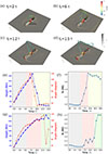 |
Fig. 12. Magnetic reconnection in eruption process. Panels (a)–(d) show the evolution of two typical flux-rope-field lines at the initial state. The bottom plane shows the distribution of Jz, which is overlaid by the temperature distribution with the translucent contours. Panels (e) and (g) show the temporal evolution of the apex height and rotation angle while panels (f) and (h) show the temporal evolution of the maximum temperature of the yellow/cyan field line, respectively. Different color bands represent different stages (see Section 4.3). |
To further investigate the effects of magnetic reconnection on the field-line connectivity, we computed the apex height, the angle with respect to the y-axis, and the maximum temperature along each field line to follow the thermodynamic response of the plasma. Figures 12e and 12f show the evolution of the yellow field line, which can be divided into three stages. In the first stage (gray bands), the maximum temperature along the field line decreases slightly, corresponding to adiabatic expansion as the apex height gradually increases. During this phase, the flux rope rotates with an almost linear correlation between rotation angle and height. Following this (red bands), the maximum temperature increases sharping, accompanied by a rapid rotation and a sudden decrease in height. Specifically, the apex height drops from 150 Mm to 20 Mm within 4 τ, indicating the transition from a flux-rope field line to a flare-loop field line. These provide clear evidence of magnetic reconnection involving the flux rope, specifically ar − rf reconnection geometry as described by Aulanier & Dudík (2019). This reconnection geometry occurs when an inclined arcade (a) field line reconnects with the leg of the erupting flux rope (r), creating a new flux-rope (r) field line rooted far away from the original flux-rope anchorage location and a flare (f) loop. This is summarized by the acronym ar − rf.
Similarly, Figures 12g and 12h show that the cyan field line also undergoes three stages, with the first two stages resembling those of the yellow line. However, in the third stage, one of its footpoints migrates into the toroidal polarity (PT), leading to a pronounced increase in temperature and rotation angle. Compared to low-lying flare loops, the flare loops formed by reconnection between the flux rope and overlying fields are longer, higher lying, and more twisted. The occurrence of such a reconnection indicates the breakup of the rising flux rope and the confinement of the eruption.
5. Forward modelings: Thermal and nonthermal
5.1. Manifestations on EUV radiation images
To investigate the observational manifestations of solar eruptions in this magnetic configuration, we forward-modeled the simulation results using the temperature and density distributions to synthesize EUV images at 94 Å as observed from the top, side, and front. In particular, the simulated temperature is scaled by an amplification factor in order to enhance the coronal emission response in high-temperature wavelength channels. Given that the coronal opacity is typically much less than unity, we adopted the optically thin approximation, considering only emission and neglecting absorption. The synthesis includes two steps. First, the emissivity in each cell is computed as  . The synthesized image is then obtained by integrating this emissivity along the line of sight. The Gλ(T) denotes the temperature response function of the EUV passband. For example, the G94(T) can be obtained from the SDO/AIA instrument response functions.
Figure 13a illustrates the evolution of flare ribbons and their associated dimmings. The ribbon dynamics proceed in two stages. In the first stage, the flare ribbons elongate along the PIL, which is due to magnetic reconnection involving strong sheared fields (as provided by the external toroidal magnetic fields, as in Qiu et al. 2017). Then, the ribbons separate perpendicular to the PIL, indicating that potential magnetic fields, supplied by the poloidal polarities, increasingly participate in reconnection. The hooked structures at the ribbon ends remain only partially closed, owing to the relatively low twist number of the flux rope2. In addition, two conjugated dark dimmings appear within the hooks and expand outward during the eruption, which is in accordance with the evolution of QSLs and the twist number shown in Figures 3 and 6. In the later stage of the eruption, two dot-like ribbons form at the far ends of the flux rope, situated at the borders of the toroidal polarities. These ribbons result from reconnection between the flux rope and the predominantly toroidal external magnetic field.
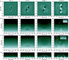 |
Fig. 13. Synthesized EUV 94 Å radiation images viewed from the (a) top, (b) front, and (c) side. The zoomed-in images in Panels (b) and (c) at t = 14 indicate the plasma blobs due to magnetic reconnection between the flux rope and the overlying toroidal fields. Panel (d) displays the temporal evolution of post-flare loops. Pink and red lines at t = 14 (bottom right panel) indicate the formed highly-sheared arcades and the underlying flare loops, which are formed due to magnetic reconnection from two groups of sheared arcades (pink lines at t = 8). The associated movie is available online. |
Figures 13b–d present synthesized EUV images from the end and side perspectives, respectively. Although the eruption remains confined in our model, the end-view images (Figure 13b) still exhibit the characteristic three-part structure of a CME: a bright leading front, a dark cavity, and a bright core, with flare loops visible beneath. By t = 14τ in Figure 13b, a plasma blob (pink circle in the zoomed-in view) appears in the upper right region of the dome-like structure. This feature serves as an observational signature of external reconnection involving the flux rope, consistent with previous observations (Li et al. 2016, 2023).
From the side view (Figure 13c), two downward-curved sheared arcades are visible beneath the dark cavity at t = 3τ. These two sheared arcades subsequently reconnect, forming an extended hot arcade along with underlying flare loops. Figure 13d provides a zoomed-in view below 50 Mm, where the flare-loop formation is traced with pink and red lines. The reconnection between the two groups of sheared arcades (pink lines) gives rise to high-lying flare loops that collectively display a transient “cowboy-hat” morphology, characterized by central loops that arch higher than those on either side.
Figure 14 shows the magnetic structure of flare loops and the synthesised 304 Å images viewed from the top. The highly sheared arcades connect the two bright regions, where the temperature is higher than the broken flux rope. One footpoint of the broken flux rope is anchored in dimming areas, whereas the other footpoint connects to the border of the dimming. The underlying flare loops exhibit a cowboy-hat morphology, in which the central portion (the hat crown) is elevated above both ends. Notably, the loop ends, corresponding to the hat brim, rise higher than the intermediate section between the brim and the crown. This configuration results from ar − rf reconnection between the flux-rope field lines and the surrounding sheared arcades (Lörinčík et al. 2021). As a result, the analysis based on synthesized EUV images and magnetic fields indicates that “cowboy-hat” morphology of the global set of flare loops is one manifestation of reconnection involved in the eruption located within the toroidal magnetic cage. It is worth noting that the cowboy-hat morphology is an ensemble of flare loops formed with different reconnection geometries rather than an individual loop.
 |
Fig. 14. Magnetic structure of flare loops and the synthesized radiation images. Panels (a) and (b) show the field lines traced from the bright regions in synthesized 304 Å radiation images viewed from the top, in which the field lines are color-coded by the temperature. Panel (c) shows the structure of post-flare loops and the comparison with synthesized 94 Å images viewed from the side. |
5.2. Nonthermal response of electron acceleration: Hard X-ray sources
To investigate the nonthermal response during the eruption, we employed the test particle method based on the guiding-center approximation (GCA) within the AMRVAC framework to study electron acceleration in the MHD environment. As described by Bacchini et al. (2024) and Wu et al. (2025), the GCA method is governed by six equations: the evolution of the guiding-center position (R), the parallel velocity component (u||), and the conservation of the magnetic moment (μ) (see Appendix C for more details). Particle acceleration is primarily driven by direct electric fields, as well as curvature, polarization, mirror, and relativistic drifts in the solar environment. The direct electric field E is defined as −v × B + ηJ, where η = 5 × 10⁻⁶ in normalized units. For more details on the GCA method, see Bacchini et al. (2024) and Wu et al. (2025). In our simulation, 5 × 10⁵ electrons following a Maxwellian velocity distribution with a temperature of T = 1 MK are injected into the magnetic-field environment provided by the MHD model, uniformly distributed across all cells, which are not related to any MHD quantities. The hard X-ray sources are synthesized using the bremsstrahlung thick-target model (Zhou et al. 2016).
Figure 15 shows the hard X-ray sources overlaid on the bottom distribution of temperature, EUV 94 Å images, and normal electric currents. At t = 3τ, hard X-ray sources with energies exceeding 50 keV are distributed in both the positive-polarity regions (associated with DCs) and the negative-polarity regions (associated with RCs), with a spectral index of –4.39. Electrons in the 25–50 keV range are deposited in flux-rope footpoints, straight ribbons, and RC. By contrast, at t = 15τ, hard X-ray sources above 50 keV are primarily deposited in RC regions, indicating that RC regions have become the dominant sites of energetic particle (> 50 keV) acceleration, and the spectral index becomes softer at −5.95. The softening of the energy spectrum between the two snapshots indicates a reduction in high-energy electrons, which may be associated with the decrease in the footpoint electric current.
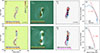 |
Fig. 15. Hard X-ray sources and electron spectra precipitating at the bottom boundary. The top and bottom rows correspond to t = 3 and 14 τ, respectively. Panels (a, e), (b, f), and (c, g) display the HXR sources (blue/yellow and red contours) overlaid on the bottom temperature distribution, synthesized EUV 94 Å emissions and vertical electric current, respectively. Panels (d) and (h) present the spectrum of electrons precipitating at the bottom boundary at t = 3 and 14 τ, respectively. |
Furthermore, the spatial distributions of energetic electrons, heated regions, and flare ribbons seen in synthesized EUV images are not co-spatial, revealing a divergence between thermal and nonthermal responses3. The heated regions, corresponding to bright flare ribbons, are mainly co-spatial with the DC regions (see Figure 7), whereas the > 50 keV electrons are primarily deposited in the RC regions. This spatial discrepancy reflects the distinct roles of return currents in plasma heating (via Joule heating) versus electron acceleration. In particular, the thermal responses, such as EUV emissions and the temperature distribution at the bottom boundary, exhibit a symmetric pattern, whereas the hard X-ray sources display pronounced asymmetry, as reported by Jin & Ding (2007), Naus et al. (2022), and Shi et al. (2024).
Regarding the enhanced electron acceleration in the return-current region, it is found that the electrons are accelerated efficiently in return currents. In the toroidal magnetic cage configuration, a current sheet beneath the flux rope fails to develop efficiently during a failed eruption. Instead, the QSLs between the flux rope and the surrounding magnetic field become more pronounced, corresponding to regions of enhanced return current. The magnetic structures carrying the return current occupy a substantially larger area than those associated with the direct current, as shown in Figure 10. Consequently, a larger population of electrons is trapped and accelerated along the longer return-current field lines. In addition, the current intensity in the return-current region is comparable to that of the direct-current region, indicating that the acceleration efficiency in the return-current channels is likewise significant.
6. Discussions
6.1. The role and magnetic properties of return current in the dynamics of flux rope
Previous studies have shown that electric-current neutralization (quantified as |DC/RC|) serves as a reliable indicator for determining the success or failure of a solar eruption (Liu et al. 2017, 2024). A positive correlation has been found between CME activity and the degree of current non-neutralization in these studies, implying that return currents play a critical role in constraining CME production. Nevertheless, we still need to know (1) which magnetic configurations are prone to producing significant return currents and (2) how return currents physically act to inhibit CME production.
Regarding the magnetic conditions that favor the generation of return currents, comparisons between the FR-PT and FR-P models indicate that external toroidal fields can induce strong return currents, reducing |DC/RC| ratio from about 30 to 10. As shown in Figures 7 and A.2, the presence of toroidal magnetic fields results in substantial return currents concentrated around the toroidal polarities. This is consistent with Duan et al. (2024), where it was reported that the degree of current neutralization in an active region is positively correlated with its magnetic non-potentiality. In our modeling, the inclusion of toroidal magnetic fields naturally reduces the twist of the core fields while enhancing the background magnetic component, thereby leading to a more current-neutralized configuration. In addition, the return currents are mainly distributed around the hooked structure at the ribbon ends rather than along their straight parts, as shown in Janvier et al. (2014).
Our results show that the magnetic properties of return current differ between the toroidal and poloidal polarities (Figure 8). The DC–RC transition point corresponds to a maximum in Bh near poloidal polarities but to a minimum in Bh around toroidal polarities. Magnetic field lines originating from poloidal polarities are more twisted (cyan lines in Figure 10), corresponding to a larger Bh field compared to that around toroidal polarities (magenta lines in Figure 10). It should be emphasized that the conclusions here are based on the TDm model, meaning that this work cannot capture how return currents are induced in a temporal evolution forming the magnetic configuration. As shown in Chintzoglou et al. (2019), the collisional shearing motions of two emerging flux tubes may produce the toroidal magnetic cage configuration illustrated here. In future work, we intend to employ observational data-driven simulations to investigate mechanisms of return-current generation in real active regions.
Regarding the role of return currents in confining eruptions, we show that those surrounding the toroidal polarities produce a downward Lorentz force (Figure 10). This force arises from the interaction between the return currents and the overlying toroidal magnetic field (Figure 9), which acts to restrain the rising of the flux rope and thereby leads to confined flares. In contrast, the Lorentz force from return currents around poloidal polarities is directed upward. This reveals the effects of the return current in governing the dynamics of the flux rope.
In summary, our simulations provide a self-consistent explanation for why active regions with more neutralized currents (lower |DC/RC| ratios) are more prone to forming confined flares (Liu et al. 2017); the downward Lorentz force generated by return currents around toroidal polarities suppresses the ascent of the flux rope. These results suggest a potential link between magnetic structure (toroidal vs. poloidal fields), current neutralization (|DC/RC|), and CME activity (success vs. failure eruptions), a relationship that could be further tested through future statistical studies.
6.2. Failed eruptions associated with filament rotation
Intriguingly, many failed eruptions are closely associated with large-angle rotations of filaments or flux ropes (Ji et al. 2003; Török & Kliem 2005; Amari et al. 2018; Zhou et al. 2019; Jiang et al. 2023; Guo et al. 2024; Zhang et al. 2024). Zhou et al. (2019) conducted a statistical analysis and found that all filaments associated with large-angle rotation in their sample ultimately halted at heights where decay index n exceeded the commonly used torus-instability threshold of 1.5, indicating that the overlying poloidal field could not restrain the ascent of eruptive flux rope. These observations raise the two key questions. We need to know (1) why eruptions with large-angle filament rotation so often fail and (2) why the decay index at the halt height is usually above 1.5 for such events.
Our simulation results provide a self-consistent explanation for these issues. As shown in Figure 11, the lateral Lorentz force driving the flux-rope rotation is mainly contributed by external toroidal magnetic fields (J × BT), rather than the flux rope itself (J × BFR) or the external poloidal field (J × BP). This finding is consistent with the parameter survey of Kliem et al. (2012) and the Lorentz-force torque analysis of Zhou et al. (2023), which demonstrates that the external sheared/toroidal field is the primary driver of flux-rope rotation. Zhang et al. (2024) further demonstrated that the rotation angle of a flux rope is not strongly correlated with its twist number prior to the eruption. These indicate that kink instability, which arises from the flux-rope self-force itself, is not the main driver of flux-rope rotation. In other words, kink instability can act as a trigger for the initiation of flux rope eruptions (such as to trigger slow-rise phase before the impulsive phase), but not as the driver governing their rotation during eruption. We therefore suggest that large-angle rotation should not be regarded as an indicator that an eruption is driven by kink instability. Instead, external toroidal fields aligned with the flux-rope axis are the dominant factor controlling flux-rope rotation. The other effect of the external toroidal field is that it produces a downward Lorentz force, which constrains the eruption. Thus, external toroidal fields can both suppress the rising of the eruptive flux rope and drive its rotation, explaining why filament rotation and failed eruptions are frequently observed together. Additionally, we performed a set of benchmark runs varying the toroidal magnetic-field strength to examine how solar eruptions depend on it in Appendix D. It is found that the rotation angle increases as the external toroidal field becomes stronger. Moreover, when the toroidal field is sufficiently strong, the eruption is suppressed and the system transitions to a failed-eruption regime. Overall, these results suggest that a stronger external toroidal field tends to enhance flux-rope rotation while also making confinement, and hence failed eruptions, more likely.
Regarding the second issue, our simulations indicate that magnetic reconnection between the flux rope and overlying toroidal fields ultimately results in its destruction. In this scenario, reconnection-induced disruption is the primary mechanism restraining the eruption (Jiang et al. 2023). Furthermore, the constraining force is mainly due to the toroidal-field-induced tension force (Myers et al. 2015, 2016), rather than the poloidal-field-induced strapping force, which accounts for why the decay index at the stopping height often exceeds 1.5.
6.3. Flare loops as a proxy for predicting CME activity
Generally, confined and eruptive flares are classified based on the presence or absence of CMEs detected by coronagraphs. However, this criterion can be unreliable for eruptions occurring near the solar disk center or for slow CMEs. In such cases, the observational signatures in the source regions, such as flare ribbons and loops, become essential to distinguish between successful and failed eruptions.
To this end, we compare the morphology of flare ribbons in confined (FE-PT) and eruptive (FE-P) flares in Figure 16 and Figure A.3, as traced from the bottom QSLs. In the confined flare case, magnetic reconnection produces three distinct structures from bottom to top: (1) short underlying flare loops traced from the inner dynamic QSLs; (2) highly sheared loops anchored at both ends of the QSLs around the toroidal polarities; and (3) overlying broken twisted loops with one footpoint at the pre-eruptive flux-rope location and the other at the outer QSL boundary near toroidal polarities.
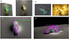 |
Fig. 16. Panels (a) and (v) show representative field lines traced from the bottom QSLs (red). Cyan and yellow lines denote the eruptive flux rope and the underlying flare loops, while green lines indicate the strongly sheared arcades connecting the two toroidal polarities. Pink curves mark the PILs on the bottom boundary. Panel (c) compares flare loops in simulations with corresponding observations. Panels (d) and (e) compare the underlying flare loops between the confined (pink lines) and eruptive cases (green lines). Pink and green curves denote the PILs on the bottom boundary for the confined and eruptive cases, respectively. |
To evaluate how well our simulation reproduces observations, we compared the modeled flare loops with those of a well-studied confined flare (Figure 16c), also referred to as a “magnetic cage” (Jiang et al. 2016; Amari et al. 2018). It is seen that both the simulation and observations exhibit strongly sheared low-lying loops and multiple ribbons (heated regions). Figures 16d-f present the ribbons and loops of the eruptive flare. In contrast to the more complex structure in the confined flare case, the eruptive flare displays a typical two-ribbon pattern in the QSLs together with saddle-like flare loops (Lörinčík et al. 2021), where the loop ends are elevated relative to the central. This geometry results from ar–rf reconnection between flux-rope field lines rooted at the hook and the ambient arcade field lines (Aulanier & Dudík 2019). As shown in Figure 16f, the modeled flare loops closely match the observations very well. These comparisons with observations suggest that our data-inspired models are capable of reflecting real-world observations.
The flare loops in confined and eruptive flares show different morphologies, making them a useful proxy to predict CME activity. In successful eruptions, flare loops typically display a saddle-like shape with a central dip. However, in confined flares they form a cowboy-hat shape, with the central loops elevated relative to the sides. Moreover, despite having nearly co-spatial central PILs (pink and green lines in Figure 16d), the two cases differ significantly in terms of the shearing degree in flare loops; flare loops in confined flares are more strongly sheared (pink arrow) than those in the eruptive case (green arrow). These results suggest that the morphology and shearing degree of flare loops can serve as diagnostic indicators: strongly sheared, cowboy-hat-shaped loops are associated with confined flares, while weakly sheared, saddle-shaped loops are characteristic of successful eruptions. It should be noted that observations have shown that photospheric magnetic fields typically exhibit larger shear angles, with non-neutralized electric currents in successful eruptions (Liu et al. 2017, 2024). In this work, however, the shear degree refers to the geometry of the flare loops rather than the photospheric magnetic field, which reflects the shearing degree of coronal magnetic fields rather than the photosphere. These results imply that accurately quantifying the degree of shear in coronal magnetic fields is crucial for distinguishing between eruptive and confined flares. Moreover, the cowboy-hat-shaped flare loops are transient, relaxing into arch-like structures within a few Alfvén crossing times. This places stringent constraints on observations: to minimize relaxation effects, measurements should be obtained as close as possible to the flare peak, while the high temperatures of newly reconnected flare loops favor observations in hot channels such as 94 and 131 Å.
7. Summary
In this work, we investigated the physical processes of solar eruptions in a configuration of a toroidal magnetic cage, with particular emphasis on the confined mechanisms and the observational manifestations. Figure 17 summarizes the key physical processes of the toroidal magnetic cage, its role in driving failed eruptions, and the corresponding observational manifestations. Our simulations demonstrate that return currents play a critical role in restricting the rise of the eruptive flux rope, providing an explanation for the tendency of confined flares to occur preferentially in current-neutralized active regions. In addition, by comparing successful and failed eruption cases, we show that the shearing degree and the morphology of flare loops can serve as useful indicators to determine CME activity. These are described below.
-
Confined mechanisms: Our results reproduce the failure of a torus-unstable flux rope constrained by overlying toroidal magnetic fields, namely the toroidal magnetic cage. A comparison with a control experiment excluding toroidal polarities reveals that external toroidal magnetic fields play a crucial role in producing confined flares. On the one hand, the return current around toroidal polarities induces a significant downward Lorentz force above the flux rope, which suppresses the flux rope’s ascent, even as magnetic reconnection continues beneath it. On the other hand, the toroidal fields drive the rotation of the flux rope, which results in the reconnection between the rotating flux rope and the overlying toroidal magnetic fields. This ultimately causes the destruction of the eruptive flux rope. The rotation angle of the flux rope increases with the strength of the toroidal magnetic field, and the eruption becomes confined when the toroidal field is sufficiently strong. These two effects of toroidal fields provide a self-consistent explanation for why filament eruptions associated with large-angle rotation are often accompanied by failed eruptions.
-
Observational manifestations in thermal and nonthermal emissions: based on simulation results, we synthesized both thermal (EUV emissions from plasma temperature and density) and nonthermal (hard X-ray sources from energetic electrons) during the eruption. The flare ribbons exhibit a multi-ribbon shape with a clockwise rotation, and two bright kernels appear near the toroidal polarities in the final stage of the eruption. The flare loops consist of underlying cowboy-hat-like loops, strongly sheared arcades connecting toroidal polarities, and the overlying broken flux rope accompanied by plasma blobs above. The hard X-ray sources are mainly spatially displaced from one EUV flare ribbon, reflecting differences in plasma heating and electron acceleration sites. Moreover, in the late stage of the eruption, the majority of energetic electrons above 50 keV are deposited along the return current ribbon, where the plasma is only weakly heated.
-
Proxy for distinguishing CME activity: Our results suggest that the morphology and shearing angle of the flare angle can serve as reliable diagnostics for distinguishing between confined and eruptive flares. In confined flares, flare loops display a relatively transient cowboy-hat shape, with the central part elevated above both ends. By contrast, eruptive flares show a saddle-like shape, where the loops at both ends rise higher than the center. They are expected to be observed near the flare peak time in the high-temperature channel. Moreover, the shearing degree of flare loops, reflecting the shearing degree of coronal magnetic fields rather than the photosphere, in confined flares is considerably stronger than in eruptive flares. Consequently, the shearing degree of flare loops serves as a useful predictor of CME activity, with loops oriented nearly perpendicular to the PIL being more likely to produce CMEs.
 |
Fig. 17. Key physical processes and observational manifestations of failed eruptions in toroidal magnetic cage. |
In summary, this study provides a systematic investigation of the magnetic cage in constraining solar eruptions, elucidating the coupled roles of the production of downward Lorentz force (Zhong et al. 2021; Zhang et al. 2024; Guo et al. 2024), flux-rope rotation (Kliem et al. 2012; Zhou et al. 2023; Zhang et al. 2024), and external magnetic reconnection (Li et al. 2016; Chen et al. 2023; Jiang et al. 2023; Li et al. 2025). We show that external toroidal magnetic fields can induce return currents, whose associated downward Lorentz force acts to suppress the eruption. However, the present analysis is based on an idealized magnetic configuration and therefore requires further validation. Specifically, the TDm model employed here does not address the origin of the return current, that is, whether it arises from flux emergence or from photospheric flows. Resolving this issue will require more realistic, observational-data-driven simulations and comprehensive radiative MHD modeling. Furthermore, the conclusion that return currents can produce a substantial downward Lorentz force should also be tested in such realistic models. Finally, the comparative analysis of confined and eruptive flare cases suggests that the morphology and shearing degree of flare loops may serve as a diagnostic parameter for distinguishing between these two types. Determining the threshold shear angle of flare loops that distinguishes confined flares from eruptive flares should be a key objective of future dedicated-parameter surveys.
Data availability
Movies associated to Figs 2, 7, and 13 are available at https://www.aanda.org
Acknowledgments
We are vert grateful to the discussions with Chen Xing and Xiaomeng Zhang at Nanjing University. J.H.G., P.F.C., and Y.G. are supported by the National Key R&D Program of China (2020YFC2201200, 2022YFF0503004), NSFC (12503063, 12127901) and the China National Postdoctoral Program for Innovative Talents fellowship under Grant Number BX20240159. SP is funded by the European Union. However, the views and opinions expressed are those of the author(s) only and do not necessarily reflect those of the European Union or ERCEA. Neither the European Union nor the granting authority can be held responsible. His project (Open SESAME) has received funding under the Horizon Europe programme (ERC-AdG agreement No 101141362). These results were also obtained in the framework of the projects C16/24/010 C1 project Internal Funds KU Leuven), G0B5823N and G002523N (WEAVE) (FWO-Vlaanderen), and 4000145223 (SIDC Data Exploitation (SIDEX2), ESA Prodex). The numerical calculations in this paper were performed in the cluster system of the High Performance Computing Center (HPCC) of Nanjing University.
References
- Amari, T., Canou, A., Aly, J.-J., Delyon, F., & Alauzet, F. 2018, Nature, 554, 211 [NASA ADS] [CrossRef] [Google Scholar]
- Aulanier, G., & Dudík, J. 2019, A&A, 621, A72 [NASA ADS] [CrossRef] [EDP Sciences] [Google Scholar]
- Aulanier, G., Pariat, E., Démoulin, P., & Devore, C. R. 2006, Sol. Phys., 238, 347 [NASA ADS] [CrossRef] [Google Scholar]
- Aulanier, G., Török, T., Démoulin, P., & DeLuca, E. E. 2010, ApJ, 708, 314 [Google Scholar]
- Aulanier, G., Janvier, M., & Schmieder, B. 2012, A&A, 543, A110 [NASA ADS] [CrossRef] [EDP Sciences] [Google Scholar]
- Bacchini, F., Ruan, W., & Keppens, R. 2024, MNRAS, 529, 2399 [NASA ADS] [CrossRef] [Google Scholar]
- Berger, M. A., & Prior, C. 2006, J. Phys. A, 39, 8321 [Google Scholar]
- Chen, P. F. 2011, Liv. Rev. Sol. Phys., 8, 1 [Google Scholar]
- Chen, P. F., Su, J. T., Guo, Y., & Deng, Y. Y. 2012, Chin. Sci. Bull., 57, 1393 [Google Scholar]
- Chen, J., Cheng, X., Kliem, B., & Ding, M. 2023, ApJ, 951, L35 [NASA ADS] [Google Scholar]
- Chintzoglou, G., Zhang, J., Cheung, M. C. M., & Kazachenko, M. 2019, ApJ, 871, 67 [NASA ADS] [CrossRef] [Google Scholar]
- Dai, Z. G., Wang, X. Y., Wu, X. F., & Zhang, B. 2006, Science, 311, 1127 [NASA ADS] [CrossRef] [Google Scholar]
- Démoulin, P., Henoux, J. C., Priest, E. R., & Mandrini, C. H. 1996a, A&A, 308, 643 [Google Scholar]
- Démoulin, P., Priest, E. R., & Lonie, D. P. 1996b, J. Geophys. Res., 101, 7631 [Google Scholar]
- Duan, A., Jiang, C., He, W., et al. 2019, ApJ, 884, 73 [NASA ADS] [CrossRef] [Google Scholar]
- Duan, A., Xing, Y., & Jiang, C. 2024, Res. Astron. Astrophys., 24, 075005 [Google Scholar]
- Fan, Y., & Gibson, S. E. 2007, ApJ, 668, 1232 [Google Scholar]
- Gardiner, T. A., & Stone, J. M. 2005, J. Comput. Phys., 205, 509 [NASA ADS] [CrossRef] [Google Scholar]
- Green, L. M., Kliem, B., Török, T., van Driel-Gesztelyi, L., & Attrill, G. D. R. 2007, Sol. Phys., 246, 365 [NASA ADS] [CrossRef] [Google Scholar]
- Guo, Y., Ding, M. D., Schmieder, B., et al. 2010, ApJ, 725, L38 [Google Scholar]
- Guo, Y., Xia, C., Keppens, R., & Valori, G. 2016, ApJ, 828, 82 [NASA ADS] [CrossRef] [Google Scholar]
- Guo, J. H., Ni, Y. W., Guo, Y., et al. 2024, ApJ, 961, 140 [NASA ADS] [CrossRef] [Google Scholar]
- Janvier, M., Aulanier, G., Pariat, E., & Démoulin, P. 2013, A&A, 555, A77 [NASA ADS] [CrossRef] [EDP Sciences] [Google Scholar]
- Janvier, M., Aulanier, G., Bommier, V., et al. 2014, ApJ, 788, 60 [Google Scholar]
- Ji, H., Wang, H., Schmahl, E. J., Moon, Y. J., & Jiang, Y. 2003, ApJ, 595, L135 [NASA ADS] [CrossRef] [Google Scholar]
- Jiang, C., Wu, S. T., Yurchyshyn, V., et al. 2016, ApJ, 828, 62 [NASA ADS] [CrossRef] [Google Scholar]
- Jiang, C., Chen, J., Duan, A., et al. 2021a, Front. Phys., 9, 575 [Google Scholar]
- Jiang, C., Feng, X., Liu, R., et al. 2021b, Nat. Astron., 5, 1126 [NASA ADS] [CrossRef] [Google Scholar]
- Jiang, C., Duan, A., Zou, P., et al. 2023, MNRAS, 525, 5857 [NASA ADS] [CrossRef] [Google Scholar]
- Jin, M., & Ding, M. D. 2007, A&A, 471, 705 [NASA ADS] [CrossRef] [EDP Sciences] [Google Scholar]
- Jing, J., Liu, C., Lee, J., et al. 2018, ApJ, 864, 138 [NASA ADS] [CrossRef] [Google Scholar]
- Keppens, R., Popescu Braileanu, B., Zhou, Y., et al. 2023, A&A, 673, A66 [NASA ADS] [CrossRef] [EDP Sciences] [Google Scholar]
- Kilpua, E. K. J., Pomoell, J., Price, D., Sarkar, R., & Asvestari, E. 2021, Front. Astron. Space Sci., 8, 35 [NASA ADS] [CrossRef] [Google Scholar]
- Kliem, B., Török, T., & Thompson, W. T. 2012, Sol. Phys., 281, 137 [NASA ADS] [Google Scholar]
- Li, L., Zhang, J., Peter, H., et al. 2016, Nat. Phys., 12, 847 [Google Scholar]
- Li, T., Chen, A., Hou, Y., et al. 2021, ApJ, 917, L29 [NASA ADS] [CrossRef] [Google Scholar]
- Li, T., Sun, X., Hou, Y., et al. 2022, ApJ, 926, L14 [NASA ADS] [CrossRef] [Google Scholar]
- Li, Z. F., Cheng, X., Ding, M. D., et al. 2023, A&A, 673, A83 [NASA ADS] [CrossRef] [EDP Sciences] [Google Scholar]
- Li, L., Song, H., Hou, Y., et al. 2025, ApJ, 979, 113 [Google Scholar]
- Liu, R., Kliem, B., Titov, V. S., et al. 2016, ApJ, 818, 148 [Google Scholar]
- Liu, Y., Sun, X., Török, T., Titov, V. S., & Leake, J. E. 2017, ApJ, 846, L6 [NASA ADS] [CrossRef] [Google Scholar]
- Liu, Y., Török, T., Titov, V. S., et al. 2024, ApJ, 961, 148 [NASA ADS] [CrossRef] [Google Scholar]
- Lörinčík, J., Dudík, J., & Aulanier, G. 2021, ApJ, 909, L4 [Google Scholar]
- Meng, Y., Lin, J., Zhang, L., et al. 2014, ApJ, 785, 62 [Google Scholar]
- Myers, C. E., Yamada, M., Ji, H., et al. 2015, Nature, 528, 526 [Google Scholar]
- Myers, C. E., Yamada, M., Ji, H., et al. 2016, Phys. Plasmas, 23, 112102 [NASA ADS] [CrossRef] [Google Scholar]
- Naus, S. J., Qiu, J., DeVore, C. R., et al. 2022, ApJ, 926, 218 [CrossRef] [Google Scholar]
- Nindos, A., Patsourakos, S., Vourlidas, A., & Tagikas, C. 2015, ApJ, 808, 117 [Google Scholar]
- Priest, E. R., & Démoulin, P. 1995, J. Geophys. Res., 100, 23443 [NASA ADS] [CrossRef] [Google Scholar]
- Qiu, J., Longcope, D. W., Cassak, P. A., & Priest, E. R. 2017, ApJ, 838, 17 [Google Scholar]
- Schmieder, B., Guo, J., & Poedts, S. 2024, Rev. Mod. Plasma Phys., 8, 27 [Google Scholar]
- Shi, G., Feng, L., Chen, J., et al. 2024, Sol. Phys., 299, 104 [Google Scholar]
- Teraoka, K., Yamasaki, D., Kawabata, Y., Imada, S., & Shimizu, T. 2025, ApJ, 983, 126 [Google Scholar]
- Thalmann, J. K., Su, Y., Temmer, M., & Veronig, A. M. 2015, ApJ, 801, L23 [NASA ADS] [CrossRef] [Google Scholar]
- Titov, V. S., & Démoulin, P. 1999, A&A, 351, 707 [NASA ADS] [Google Scholar]
- Titov, V. S., Hornig, G., & Démoulin, P. 2002, J. Geophys. Res. (Space Phys.), 107, 1164 [Google Scholar]
- Titov, V. S., Török, T., Mikic, Z., & Linker, J. A. 2014, ApJ, 790, 163 [NASA ADS] [CrossRef] [Google Scholar]
- Titov, V. S., Downs, C., Mikić, Z., et al. 2018, ApJ, 852, L21 [NASA ADS] [CrossRef] [Google Scholar]
- Török, T., & Kliem, B. 2005, ApJ, 630, L97 [Google Scholar]
- Török, T., Berger, M. A., & Kliem, B. 2010, A&A, 516, A49 [NASA ADS] [CrossRef] [EDP Sciences] [Google Scholar]
- Tsurutani, B. T., Zank, G. P., Sterken, V. J., et al. 2023, IEEE Trans. Plasma Sci., 51, 1595 [CrossRef] [Google Scholar]
- Wang, Y., & Zhang, J. 2007, ApJ, 665, 1428 [Google Scholar]
- Wang, D., Liu, R., Wang, Y., et al. 2017, ApJ, 843, L9 [Google Scholar]
- Wu, H., Guo, Y., Keppens, R., et al. 2025, ApJ, 992, 81 [Google Scholar]
- Xia, C., Teunissen, J., El Mellah, I., Chané, E., & Keppens, R. 2018, ApJS, 234, 30 [Google Scholar]
- Xing, C., Aulanier, G., Schmieder, B., Cheng, X., & Ding, M. 2024, A&A, 682, A3 [NASA ADS] [CrossRef] [EDP Sciences] [Google Scholar]
- Xu, Y., Zhu, J., & Guo, Y. 2020, ApJ, 892, 54 [NASA ADS] [CrossRef] [Google Scholar]
- Zhang, X. M., Guo, J. H., Guo, Y., Ding, M. D., & Keppens, R. 2024, ApJ, 961, 145 [NASA ADS] [CrossRef] [Google Scholar]
- Zhao, J., Gilchrist, S. A., Aulanier, G., et al. 2016, ApJ, 823, 62 [Google Scholar]
- Zhong, Z., Guo, Y., & Ding, M. D. 2021, Nat. Commun., 12, 2734 [NASA ADS] [CrossRef] [Google Scholar]
- Zhou, X., Büchner, J., Bárta, M., Gan, W., & Liu, S. 2016, ApJ, 827, 94 [NASA ADS] [CrossRef] [Google Scholar]
- Zhou, Z., Cheng, X., Zhang, J., et al. 2019, ApJ, 877, L28 [NASA ADS] [CrossRef] [Google Scholar]
- Zhou, Z., Jiang, C., Yu, X., et al. 2023, Front. Phys., 11, 1119637 [Google Scholar]
- Zuccarello, F. P., Chandra, R., Schmieder, B., Aulanier, G., & Joshi, R. 2017, A&A, 601, A26 [NASA ADS] [CrossRef] [EDP Sciences] [Google Scholar]
It should be noted that these definitions are not rigid for two reasons. First, the orientations of the toroidal and poloidal components in the flux-rope coordinate system change as the rope rotates. Second, the self-force of the flux rope consists of both the hoop force (JFR, T × BFR, P) and tension force (JFR, P × BFR, T).
In principal, strong toroidal fields can decrease the twist number of the flux rope, while poloidal fields have opposite effects.
It should be noted that the feedback of energetic electrons on the MHD equation is neglected. Therefore, all heating arises solely from thermal mechanisms, including Joule heating, compression, and thermal conduction.
Appendix A: Control experiment 1: successful eruption in a magnetic configuration dominated by poloidal fields
To investigate the role of external toroidal magnetic fields on flux rope eruption, we conduct a control experiment referred to as model FR-P. In this model, we eliminate the external toroidal magnetic fields generated by NT and PT polarities while maintaining consistency with the other parameters in the benchmark case described in Section 2 (referred to as model FR-PT). In contrast to the failed eruption with significant rotation in model FR-PT, the flux rope in model FR-P ascends to a height of 300 Mm within 12 τ (Figure A.1d). Moreover, magnetic reconnection primarily occurs beneath the flux rope in model FR-P, converting overlying loops into part of the flux rope and thereby reducing their downward magnetic tension, which opposes the flux rope rise. In addition, for model FR-PT, magnetic reconnection also takes place between the rotated flux rope and the overlying toroidal magnetic fields, ultimately disrupting the flux rope and leading to its failed eruption. These differences highlight the critical role of overlying large-scale toroidal magnetic fields in triggering failed solar eruptions with significant rotation.
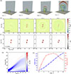 |
Fig. A.1. Evolution of the model FR-P in the eruption process. Panel (a) displays 3D magnetic structures during the eruption. The yellow and cyan lines represent the magnetic fields traced from the pre-eruptive flux-rope footpoints and the poloidal polarities, respectively. Panels (b) and (c) show the distribution of the temperature and twist on the bottom plane, respectively. Panel (d) shows the time-distance diagram of the By along the z-axis. Panel (e) shows the kinetics of the flux rope by measuring the +By front in Panel (d), wherein the blue and red lines represent the evolution of height and speed. |
Figure A.1b shows the morphology of flare ribbons, outlined by the heated regions. The modeled flare ribbons display a separated double J-shaped structure, which aligns well with the 3D standard flare model (Janvier et al. 2014). Additionally, the hooked structures at both ends of flare ribbons, typically surrounding the flux rope footpoints, become increasingly closed. This reflects an increase in the twist at the flux rope border during the eruption process due to the magnetic reconnection of the dominantly poloidal magnetic field below the erupting flux rope (Démoulin et al. 1996b; Zhao et al. 2016). In contrast, the hooked flare ribbons in model FR-PT remain relatively open, indicating a lower twist for three reasons. First, the presence of external toroidal fields reduces the ratio of poloidal to toroidal flux within the flux rope, thereby lowering its twist. Second, the magnetic field lines in the current sheet beneath the flux rope are more strongly sheared in model FR-PT. As a result, the amount of twisted flux injected into the flux rope via magnetic reconnection is also diminished. Third, 3D magnetic reconnection involving the flux rope itself can ruin its structure, further decreasing its twist.
Figure A.1c shows the distribution of the twist number on the bottom plane, indicating the footpoints of the flux rope. The areas of the flux rope footpoints increase first and then decrease, but the twist number increases during the eruption, which is significantly different from the confined eruption in model FR-PT. The increase in the flux-rope footpoint area corresponds to reconnection occurring in the arcade field lines beneath it, which converts sheared arcades into the flux rope (aa–rf),. Hereafter, a decrease in the flux-rope footpoint area reflects reconnection involving the flux rope itself, e.g., reconnection within the flux-rope field lines (rr–rf) or the reconnection between the eruptive flux rope and the overlying field lines (ar–rf), as also reported by Jiang et al. (2021a). Figures A.1d and A.1e show the kinetics of the flux rope by measuring the +By leading front of the flux rope. Its velocity increases to about 250 km s−1 at t = 6τ but subsequently starts to decrease due to the boundary issues in the finite computation domain.
The evolution of electric currents is illustrated in Figure A.2. The return current around the flux rope in the FR-P model is significantly lower compared to that in the FR-PT model. This suggests that the toroidal magnetic fields are crucial to induce the return current. Moreover, the degree of current neutralisation, represented by |DC/RC|, is significantly higher in model FR-P (∼30), so that the currents are less neutralised, compared to model FR-PT (∼9; Figure 9a). This is consistent with the statistical findings of Liu et al. (2017), Liu et al. (2024) and Duan et al. (2024), who found that the electric currents of eruptive core fields are closer to unity in confined eruptions compared to eruptive events. However, it is essential to note that the flux rope in our model is based on the TDm model, which only considers the direct current flowing through the flux rope. As a result, the neutralisation degree measured by |DC/RC| is higher than the typically observed values. Figure A.3 shows the flare loops and their comparison with observations. The flare loops in the FR-P case exhibit a pronounced saddle-like morphology, with the loops on both sides rising higher than those in the central section, consistent with the observations reported by Lörinčík et al. (2021).
 |
Fig. A.2. Evolution of the electric current during the eruption. Panels (a)–(b) display the distribution of Jx, Jy on the x − y plane, respectively. Panel (c) shows the distribution of Jz on the bottom plane. Panel (d) illustrates the temporal evolution of |DC/RC| during the eruption process. Panel (e) shows the magnetic properties (Bz, Jz and Bh) along the slit S3 in Panel (c) at t = 14. |
 |
Fig. A.3. Flare loops, QSLs, and comparisons with observations in the successful-eruption case. The yellow lines represent the flare loops, while the cyan lines correspond to the eruptive flux rope. The red line marks the PIL on the bottom plane, and the red contours denote the QSLs. |
Appendix B: Control xxperiment 2: evolution of an individual flux rope
To isolate the effects of the Lorentz force from external magnetic fields and magnetic reconnection, we remove both the external toroidal and poloidal magnetic fields while retaining the flux rope in the initial magnetic configuration, referred to as model FR. Figure B.1 presents the evolution of an individual flux rope. Initially, the flux rope undergoes slight deformation accompanied by counter-clockwise rotation, consistent with the distribution of its self-induced Lorentz force, as shown in Figure 11c, which may be related to the kink instability. Subsequently, the flux rope almost maintains a fixed morphology as it rises. Notably, the writhe number of an S-shaped curve anchored to the surface is positive when it is low-lying, but becomes negative once its apex reaches a critical height (Török et al. 2010; Xu et al. 2020). The simulation between models FR, FR-PT and FR-P indicates that the external toroidal magnetic fields are the key to inducing the rotation of the flux rope.
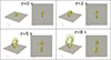 |
Fig. B.1. 3D magnetic fields of an individual flux rope during the eruption. Yellow and red lines represent the twisted field lines and the flux-rope axis, respectively. |
Appendix C: Test-particle method for solving particle motion with GCA
Here, we introduce the test-particle method implemented in the MPI-AMRVAC framework based on the GCA. This approach relies on two assumptions. First, the electron lifetime is much shorter than the evolution timescale of the coronal MHD system. Second, the electron gyro-radius and gyro-period are much smaller than the characteristic spatial and temporal scales of the large-scale MHD evolution. As such, the gyromotion of particles perpendicular to the magnetic field can be averaged out, and the particle dynamics can be described in terms of the guiding-center position (R), the motion parallel to the magnetic field (u∥), and the magnetic moment (μ = mu⊥2/2Bκ = mu⊥2/2B(1 − vE2/c2)−1/2), as follows (Bacchini et al. 2024; Wu et al. 2025):
 (C.1)
(C.1)
 (C.2)
(C.2)
 (C.3)
(C.3)
where electric field is computed from E = −v × B + ηJ, and the parallel electric field (E∥) is defined as E ⋅ B. The guiding-centre position of electrons is dominated by parallel motion (u∥), E × B drift (vE), curvature drift (vcurv), gradient drift (v∇B), polarization drift vpol, and the relativistic correction (vrel). They are described as follows:
 (C.4)
(C.4)
![Mathematical equation: $$ \begin{aligned} \boldsymbol{v}_{\text{curv}} = \frac{mc\kappa ^2}{qB} \boldsymbol{b} \times \left[ \frac{u_\parallel ^2}{\gamma } (\boldsymbol{b} \cdot \nabla ) \boldsymbol{b} + u_\parallel (\boldsymbol{v}_E \cdot \nabla ) \boldsymbol{b} \right], \end{aligned} $$](/articles/aa/full_html/2026/06/aa59355-26/aa59355-26-eq16.gif) (C.5)
(C.5)
![Mathematical equation: $$ \begin{aligned} \boldsymbol{v}_{\text{pol}} = \frac{mc\kappa ^2}{qB} \boldsymbol{b} \times \left[ u_\parallel (\boldsymbol{b} \cdot \nabla ) \boldsymbol{v}_E + \gamma (\boldsymbol{v}_E \cdot \nabla ) \boldsymbol{v}_E \right], \end{aligned} $$](/articles/aa/full_html/2026/06/aa59355-26/aa59355-26-eq17.gif) (C.6)
(C.6)
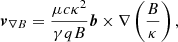 (C.7)
(C.7)
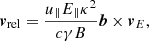 (C.8)
(C.8)
where coefficient κ is derived from  , γ is the Lorentz factor, b is the unit vector along the magnetic field direction, q is the electric charge of the particle, and c is the light speed. Regarding the parallel motion along magnetic fields, the acceleration items resulting from the curvature and gradient of magnetic fields are described by:
![Mathematical equation: $$ \begin{aligned} a_{\text{curv}} = \boldsymbol{v}_E \cdot \left[ u_\parallel (\boldsymbol{b} \cdot \nabla ) \boldsymbol{b} + \gamma (\boldsymbol{v}_E \cdot \nabla ) \boldsymbol{b} \right], \end{aligned} $$](/articles/aa/full_html/2026/06/aa59355-26/aa59355-26-eq21.gif) (C.9)
(C.9)
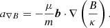 (C.10)
Appendix D: Parameter survey for the strength of toroidal magnetic fields
To investigate the role of the toroidal magnetic field strength, we perform a parameter survey by varying qt from 4qt0, 2qt0, and qt0 to 0.5qt0, 0.25qt0, and 0. The case with qt = qt0 corresponds to Case FR-PT, whereas the case with qt = 0 corresponds to Case FR-P. The three-dimensional magnetic field structures at the same time are shown in Figure D.1. It is found that the rotation angle of the flux rope increases with increasing toroidal magnetic field strength. In addition, when the toroidal magnetic field becomes sufficiently strong, the eruption turns into a failed eruption. These results confirm that the toroidal magnetic field promotes the rotation of the flux rope and can suppress the eruption when its strength is sufficiently large.
 |
Fig. D.1. Parameter survey of the toroidal magnetic-field strength. The red contours at the bottom indicate QSLs, used here as proxies for flare ribbons. The toroidal field strength decreases from panel (a) to panel (f). |
All Figures
|
Fig. 1. Visualization of the initial magnetic fields viewed from the (a) side and (b) top. The yellow, cyan, and magenta tubes represent the twisted flux rope and the overlying poloidal and toroidal magnetic fields, respectively. NP/NT and PP/PT label the negative and positive sub-photosphere magnetic charges to build the poloidal/toroidal magnetic fields, respectively. |
| In the text | |
|
Fig. 2. Height profiles of decay index computed from external total horizontal magnetic fields (Bh, blue line), poloidal fields (Bp, orange line), and toroidal fields (BT, green line). The orange and green bands indicate regions of the flux rope at initial and stopping moments, respectively. The associated movie is available online. |
| In the text | |
|
Fig. 3. Temporal evolution of (a–d) magnetic-field and (e, f) twist-number Tw distributions in the eruption process. The yellow, cyan, and pink tubes are traced from the NFR, NP, and NT polarities, respectively. The colors in the bottom and vertical planes exhibit the distributions of the Bz and Te, respectively. Panels (e) and (f) display the Tw distributions on the vertical and bottom planes, respectively. |
| In the text | |
|
Fig. 4. Temporal evolution of (a) the axial magnetic field component, By; (b) the number density, n; and (c) the temperature, Te, at t = 2, 6, 9, 15τ. The dashed line in the t = 9 column outlines the border of the flux rope (with added reconnected flux). |
| In the text | |
|
Fig. 5. Kinematics of eruptive flux rope. Panel (a) shows the time–distance diagram of the By component along the z-axis. In panel (b) the blue dots and red crosses show the evolution of height and velocity during the eruption, which are measured with the positive By front in panel (a). |
| In the text | |
|
Fig. 6. Evolution of flare ribbons depicted from the (a, c) temperature and (b, d) QSL distributions. Temporal evolution of the (a) temperature and (b) squashing degree, Q, of QSLs on the bottom plane. Panels (c) and (d) show the time–distance diagram of temperature and Q along the blue line in Panel (a3), respectively. Two wave-like fronts in Panels (a3) and (a4) correspond to the shock in Figure 4c. The artifacts of Q near the side boundaries arise from the finite size of the computational domain. However, they do not give rise to significant heating fronts, electric currents, or Lorentz forces, and thus they have only a small impact on the derived conclusions. The box size is equal to that in plots (e) and (f) of Figure 3. |
| In the text | |
|
Fig. 7. Evolution of electric current during eruption. The first (a1–a4), second (b1–b4), and third (c1–c4) rows display the distributions of Jx, Jy, and Jz, respectively, in the central vertical plane. The (d1–d4) bottom row displays the distributions of Jz in the bottom horizontal plane. The dashed red (positive Bz) and black (negative Bz) lines represent the contour lines of Bz = ±40, 20, 10, and 5 G. In regions of positive/negative Bz (red/black contours), positive/negative currents (red/blue) represent the DC system, whereas negative/positive currents (blue/red) form the RC system. The 1D slits S1 and S2 are defined in panels (d3) and (d4) by yellow and pink segments, respectively, showing the. Some averaged quantities at z = 0 within these slits are shown in Figure 8. The associated movie is available online. |
| In the text | |
|
Fig. 8. Panel (a) shows the temporal evolution of |DC/RC| in the eruption process. Panels (b) and (c) display the average magnetic properties of the direct-return currents near the poloidal polarity (S1, Figure 7d3) and the toroidal polarity (S2, Figure 7d3). The violet, orange, and brown lines represent the profiles of normal electric current (Jz), horizontal magnetic field (Bh), and normal magnetic field (Bz), respectively. |
| In the text | |
|
Fig. 9. Distribution of vertical Lorentz force in the x − z plane at the times of 2, 6, 9, and 15 τ. Panels (a)–(d) exhibit the vertical component of Lorentz force induced from total magnetic fields, flux-rope fields, external poloidal fields, and toroidal fields, respectively. |
| In the text | |
|
Fig. 10. Relationship among magnetic-field lines and the electric current, Lorentz force, and magnetic-field components. Panels (a) and (b) show the field lines traced from DC (yellow, green, cyan, and blue lines) and RC (red and magenta lines). Panel (c) shows the distribution of the vertical Lorentz force on the X-Z plane. Panel (d) displays the distribution of Jx, Jy, Bx, and By on the x-z plane. |
| In the text | |
|
Fig. 11. Distribution of lateral Lorentz force in the x-z plane at the times of 2, 6, 9, and 15 τ. Panels (a)–(c) exhibit the horizontal x component of Lorentz force induced from the flux rope itself, external poloidal fields and toroidal fields, respectively. The plane is selected at z = 50 Mm, as shown in Figure 9a. The inserted image in Panel (a) at t = 9 shows the Jz distribution and the corresponding field lines. |
| In the text | |
|
Fig. 12. Magnetic reconnection in eruption process. Panels (a)–(d) show the evolution of two typical flux-rope-field lines at the initial state. The bottom plane shows the distribution of Jz, which is overlaid by the temperature distribution with the translucent contours. Panels (e) and (g) show the temporal evolution of the apex height and rotation angle while panels (f) and (h) show the temporal evolution of the maximum temperature of the yellow/cyan field line, respectively. Different color bands represent different stages (see Section 4.3). |
| In the text | |
|
Fig. 13. Synthesized EUV 94 Å radiation images viewed from the (a) top, (b) front, and (c) side. The zoomed-in images in Panels (b) and (c) at t = 14 indicate the plasma blobs due to magnetic reconnection between the flux rope and the overlying toroidal fields. Panel (d) displays the temporal evolution of post-flare loops. Pink and red lines at t = 14 (bottom right panel) indicate the formed highly-sheared arcades and the underlying flare loops, which are formed due to magnetic reconnection from two groups of sheared arcades (pink lines at t = 8). The associated movie is available online. |
| In the text | |
|
Fig. 14. Magnetic structure of flare loops and the synthesized radiation images. Panels (a) and (b) show the field lines traced from the bright regions in synthesized 304 Å radiation images viewed from the top, in which the field lines are color-coded by the temperature. Panel (c) shows the structure of post-flare loops and the comparison with synthesized 94 Å images viewed from the side. |
| In the text | |
|
Fig. 15. Hard X-ray sources and electron spectra precipitating at the bottom boundary. The top and bottom rows correspond to t = 3 and 14 τ, respectively. Panels (a, e), (b, f), and (c, g) display the HXR sources (blue/yellow and red contours) overlaid on the bottom temperature distribution, synthesized EUV 94 Å emissions and vertical electric current, respectively. Panels (d) and (h) present the spectrum of electrons precipitating at the bottom boundary at t = 3 and 14 τ, respectively. |
| In the text | |
|
Fig. 16. Panels (a) and (v) show representative field lines traced from the bottom QSLs (red). Cyan and yellow lines denote the eruptive flux rope and the underlying flare loops, while green lines indicate the strongly sheared arcades connecting the two toroidal polarities. Pink curves mark the PILs on the bottom boundary. Panel (c) compares flare loops in simulations with corresponding observations. Panels (d) and (e) compare the underlying flare loops between the confined (pink lines) and eruptive cases (green lines). Pink and green curves denote the PILs on the bottom boundary for the confined and eruptive cases, respectively. |
| In the text | |
|
Fig. 17. Key physical processes and observational manifestations of failed eruptions in toroidal magnetic cage. |
| In the text | |
|
Fig. A.1. Evolution of the model FR-P in the eruption process. Panel (a) displays 3D magnetic structures during the eruption. The yellow and cyan lines represent the magnetic fields traced from the pre-eruptive flux-rope footpoints and the poloidal polarities, respectively. Panels (b) and (c) show the distribution of the temperature and twist on the bottom plane, respectively. Panel (d) shows the time-distance diagram of the By along the z-axis. Panel (e) shows the kinetics of the flux rope by measuring the +By front in Panel (d), wherein the blue and red lines represent the evolution of height and speed. |
| In the text | |
|
Fig. A.2. Evolution of the electric current during the eruption. Panels (a)–(b) display the distribution of Jx, Jy on the x − y plane, respectively. Panel (c) shows the distribution of Jz on the bottom plane. Panel (d) illustrates the temporal evolution of |DC/RC| during the eruption process. Panel (e) shows the magnetic properties (Bz, Jz and Bh) along the slit S3 in Panel (c) at t = 14. |
| In the text | |
|
Fig. A.3. Flare loops, QSLs, and comparisons with observations in the successful-eruption case. The yellow lines represent the flare loops, while the cyan lines correspond to the eruptive flux rope. The red line marks the PIL on the bottom plane, and the red contours denote the QSLs. |
| In the text | |
|
Fig. B.1. 3D magnetic fields of an individual flux rope during the eruption. Yellow and red lines represent the twisted field lines and the flux-rope axis, respectively. |
| In the text | |
|
Fig. D.1. Parameter survey of the toroidal magnetic-field strength. The red contours at the bottom indicate QSLs, used here as proxies for flare ribbons. The toroidal field strength decreases from panel (a) to panel (f). |
| In the text | |
Current usage metrics show cumulative count of Article Views (full-text article views including HTML views, PDF and ePub downloads, according to the available data) and Abstracts Views on Vision4Press platform.
Data correspond to usage on the plateform after 2015. The current usage metrics is available 48-96 hours after online publication and is updated daily on week days.
Initial download of the metrics may take a while.