


| Issue |
A&A
Volume 710, June 2026
|
|
|---|---|---|
| Article Number | A125 | |
| Number of page(s) | 14 | |
| Section | Numerical methods and codes | |
| DOI | https://doi.org/10.1051/0004-6361/202558655 | |
| Published online | 05 June 2026 | |
A novel method for measuring spectral lags by dynamic time warping
1
School of Physics and Electronic Science, Guizhou Normal University,
Guiyang
550001,
PR China
2
Guizhou Provincial Key Laboratory of Radio Astronomy and Data Processing, Guizhou Normal University,
Guiyang
550001,
PR China
★ Corresponding author: This email address is being protected from spambots. You need JavaScript enabled to view it.
Received:
18
December
2025
Accepted:
16
April
2026
Abstract
Context. Measuring spectral lags in gamma-ray bursts (GRBs) across different energy bands is important for studying prompt-emission physics and related applications.
Aims. We assessed the reliability and applicability of the constrained dynamic time warping (DTW) method for measuring spectral lags in GRBs.
Methods. We applied the constrained DTW method to a sample of 50 single-pulse GRBs observed by Fermi/GBM and compared the resulting spectral lags with those obtained using Gaussian peak-time fitting and the modified cross-correlation function (MCCF). We also performed simulation-based tests with known input lags to validate the method.
Results. The spectral lags derived from DTW are overall consistent with those obtained from Gaussian fitting and MCCF, with no significant differences found within 3σ. For evidently asymmetric pulses, fitting the full pulse with a symmetric Gaussian function can bias the inferred lag, while peak-focused Gaussian fitting yields results more consistent with DTW and MCCF. Simulations show that DTW can reliably recover the input lag and provide robust uncertainty estimates.
Conclusions. Dynamic time warping provides a robust and complementary approach to spectral-lag measurement in GRBs and is promising for future applications to more complex light curves and related studies such as gravitational-lensing searches.
Key words: methods: data analysis
© The Authors 2026
 Open Access article, published by EDP Sciences, under the terms of the Creative Commons Attribution License (https://creativecommons.org/licenses/by/4.0), which permits unrestricted use, distribution, and reproduction in any medium, provided the original work is properly cited.
This article is published in open access under the Subscribe to Open model. This email address is being protected from spambots. You need JavaScript enabled to view it. to support open access publication.
1 Introduction
Gamma-ray bursts (GRBs), among the most luminous cosmic explosions, are usually categorized into long-duration bursts originating from massive star core collapse and short-duration bursts from compact object mergers (e.g., Woosley & Bloom 2006; Abbott et al. 2017). The spectral lag, defined as the time delay between the arrival of low-energy and high-energy photons (with a positive lag indicating that high-energy photons arrive before low-energy ones), serves as a critical parameter in GRB physics, such as relativistic plasma motion and fireball curvature effects in fundamental radiation mechanisms (e.g., Chen et al. 2005; Sari & Piran 1997; Dermer 2004; Ukwatta et al. 2012a; Bernardini et al. 2015). In addition, spectral lag is one of the most decisive diagnostics for identifying GRBs of special origin, as exemplified by GRB 200415A, GRB 230307A, and GRB 211211A (e.g., Yang et al. 2020; Mei et al. 2022; Yang et al. 2022; Troja et al. 2022; Gompertz et al. 2023; Xiong et al. 2023; Xiao et al. 2024). Moreover, the spectral lag serves as a powerful probe for testing Lorentz invariance violation (LIV) in quantum gravity theories, where photon delays may encode quantum gravitational effects (e.g., Kostelecký & Samuel 1989; Abdo et al. 2009b,a; Wei et al. 2017; Acciari et al. 2020; Xiao et al. 2022; Lan et al. 2022).
Previous studies have shown that long GRBs generally exhibit a broader spectral-lag distribution, whereas short GRBs tend to have smaller lags, often clustering around zero (e.g., Norris & Bonnell 2006; Ukwatta et al. 2012a). However, current samples do not provide stronger than 2σ evidence that the lag distributions of short and long GRBs are drawn from different parent populations (Bernardini et al. 2015). Spectral lag alone is therefore not a definitive discriminator of GRB class or progenitor. A more robust physical classification generally requires combining prompt-emission observables with additional diagnostics, such as host-galaxy properties, redshift, burst offset from the host center, and other temporal characteristics such as the minimum variability timescale (e.g., Leibler & Berger 2010; MacLachlan et al. 2013; Fong et al. 2013; Berger 2014; Golkhou et al. 2015; Xiao et al. 2024.)
Shen et al. (2005) showed that relativistic curvature effects alone can produce observable spectral lags and energydependent pulse widths, even without invoking intrinsic spectral evolution, while Uhm & Zhang (2016) further demonstrated that spectral lags can arise naturally when the photon spectrum is curved and the emitting region undergoes bulk acceleration, linking lag measurements to relativistic jet dynamics. Beyond such geometric and kinematic effects, spectral lags can also arise from intrinsic spectral evolution of the prompt emission, as supported by time-resolved analyses and theoretical models showing that the evolution of the spectral peak and shape can generically produce energy-dependent pulse widths and soft lags in promptemission scenarios (e.g., Lu et al. 2018; Bošnjak & Daigne 2014). Spectral lag has therefore been widely used as a diagnostic of GRB prompt-emission physics and was also proposed as a possible luminosity-related observable in long GRBs (e.g., Ukwatta et al. 2010, 2012a); however, this interpretation is not universal, since the lag-luminosity correlation becomes significantly weaker when long GRBs with lags consistent with zero are included (Bernardini et al. 2015). More recently, Xiao et al. (2023) reported linear energy-dependent lags in X-ray bursts from the magnetar SGR J1935+2154, suggesting a linear temporal evolution of the temperature of the blackbody-emitting plasma.
Current measurements of spectral lag mainly adopt two approaches: the cross-correlation function (CCF; e.g., Norris et al. 2000; Ukwatta et al. 2012b; Xiao et al. 2022) and light curve fitting (e.g., Norris et al. 2005; McBreen et al. 2008; Shao et al. 2017). The CCF computes the correlation coefficient between light curves recorded in different energy bands, and the spectral lag is taken as the time shift that maximizes the correlation. This method is model-independent, as no assumption about the functional shape of the pulse is required. However, it is sensitive to individual bright pulses, and it cannot account for variations in pulse width across different energy bands (e.g., Norris et al. 2005). The light curve fitting method involves fitting each light curve with a pulse model, and the spectral lag is defined as the difference between the peak times.
This method is model-dependent, and the derived lag can change if the assumed pulse shape is incorrect. For multi-pulsed GRBs, additional ambiguity arises when several pulses overlap, because there is no unique prescription for which fitted peak to use to define the lag. Moreover, different pulses within the same GRB may exhibit different spectral lags, introducing additional systematic uncertainty.
Dynamic time warping (DTW) is a classic time-series similarity measure designed for two sequences. Its core idea is to nonlinearly “warp” the time axis so that corresponding events are optimally matched; even if the sequences are stretched, shifted, or rescaled in time, their shape resemblance can still be assessed robustly (e.g., Folgado et al. 2018; Morel et al. 2018; Lee 2019). The algorithm returns the minimum cumulative distance as the DTW distance. It not only provides the cumulative distance as a similarity measure but also generates the optimal alignment between the two time series (e.g., Strle et al. 2009; Lahreche & Boucheham 2021). This characteristic allows DTW to overcome the limitations of traditional rigid metrics such as Euclidean distance, providing great flexibility for complex time series analysis (e.g., Choi et al. 2020; Serra & Arcos 2012). Precisely due to these significant advantages, DTW has been extensively applied and expanded across numerous fields including, but not limited to, astronomy (e.g., Zhang et al. 2016; Abraham et al. 2021), speech recognition (e.g., Richter & GuÐnason 2023), and agriculture (e.g., Guan et al. 2016).
In this study, we employed DTW as a novel tool to calculate the spectral lags between light curves and compare the spectral lags obtained using the Gaussian peak and modified CCF methods. Section 2 introduces the data selection, the principles of DTW, and the methodology for calculating spectral lags using DTW. Section 3 presents a comparative analysis of the results obtained from the three distinct methods. Finally, Sect. 4 provides a summary of the study.
2 Data and methodology
2.1 Data
To facilitate direct comparison with previous methods such as the CCF and Gaussian-fitting approaches, we adopted the same sample of 50 single-pulse GRBs observed by the Fermi Gammaray Burst Monitor (Fermi/GBM; e.g., Meegan et al. 2009) and the same energy bands used by Shao et al. (2017), namely 1015, 15-22, 22-34, 34-51, 51-77, 77-116, 116-176, 176-265, and 265-400 keV. We used time-tagged event (TTE) data from the brightest NaI detector. In most cases, the time window adopted for the DTW analysis approximately follows the T90 interval of the burst. For a small number of GRBs with long and weak extended emission showing little obvious temporal structures, we further refined the window through visual inspection by excluding these nearly featureless intervals and focusing on the main burst episode with the most significant temporal variations.
2.2 Methodology
In this study, we employed DTW as a novel tool to calculate the spectral lags between the light curves. The core principle of DTW is to find an optimal alignment path between the two time series, A = (a1, a2,..., an) and B = (b1, b2,..., bm), by dynamically “warping” the time axis of one sequence so that its event timing best matches that of the other. This allows shape similarities between the two sequences to be measured through minimum cumulative distance. This principle is illustrated in the left panel of Fig. 1.
The method first involves constructing an n × m cumulative matrix D, where each element (i, j) (for 1 ≤ i ≤ n and 1 ≤ j ≤ m) corresponds to the local distance between ai and bj, defined as
 (1)
(1)
The matrix is initialized as follows: The first cell is given by
 (2)
(2)
while the first row (i > 1, j = 1) is given by
 (3)
(3)
This can only extend from left to right, indicating that the first point of B is aligned sequentially with the first i points of A.
For the first column (i = 1, j > 1),
 (4)
(4)
which can only extend from bottom to top, indicating that the first point of A is aligned sequentially with the first j points of B.
Recursive filling of the remaining elements is computed by
 (5)
(5)
where each cell takes the minimum cumulative cost from its three possible predecessors.
Backtracking proceeds by starting from the endpoint (n, m) and simply reversing the path through repeated selection of the predecessor among {(i - 1, j), (i, j - 1), (i - 1, j - 1)} that minimizes the D value. This ensures the entire reversed path remains consistent with the globally optimal substructure. “Minimum predecessor” selection is repeated until reaching (1,1).
Finally, the value D (n, m) in the top-right corner represents the minimum cumulative distance between the two time series A and B. A smaller value indicates a higher degree of similarity between the two sequences.
However, a well-known limitation of standard DTW is that it may produce pathological alignments, in which a relatively short segment in one sequence is matched to an excessively long segment in the other, resulting in physically implausible many-to-one mappings (e.g., Zhao & Itti 2018; Zhang et al. 2017). To mitigate this problem, we imposed the Sakoe-Chiba band as a global path constraint, as illustrated in the right panel of Fig. 1. Such global constraints are widely used to suppress pathological warping and improve the robustness of DTW alignment (e.g., Yu et al. 2011; Sakoe & Chiba 2003). Among them, the Sakoe-Chiba band is one of the most commonly adopted choices. Previous studies have shown that relatively narrow bands, typically no more than about 10% of the sequence length, often perform well in practice (e.g., Keogh & Ratanamahatana 2004; Ratanamahatana & Keogh 2004; Niennattrakul & Ratanamahatana 2009; Alajlan 2011). We therefore adopted a band width of 10% of the sequence length as an empirically motivated and conservative setting rather than a value formally optimized over our GRB sample.
Before applying the DTW algorithm, we estimated and subtracted the background from the Fermi/GBM light curves in each energy band, since DTW searches for similarities between light curves and band-dependent background variations could otherwise affect the alignment. We then applied the constrained DTW method to compute the spectral lags among the light curves in nine energy bands for a sample of 50 GRBs, taking the lowest-energy channel (10-15 keV) as the reference channel, RE(t), and the remaining eight higher-energy channels as comparison channels, CE(i)(t) (i = 1, 2,..., 8). Before the DTW calculation, all light curves were normalized using min-max normalization, a standard preprocessing step in time-series mining that improves comparability between sequences (e.g., Giao & Anh 2016). For a time series X = {x 1, x2,..., xn}, min-max normalization is defined as
 (6)
(6)
where min(X) and max(X) are the minimum and maximum values of the sequence, respectively, and x′i is the normalized value in the range [0,1]. This preprocessing step reduces the influence of absolute count-scale differences between the energy bands and allows the DTW alignment to focus on the relative temporal morphology of the light curves.
To determine the spectral lag, the normalized reference light curve RE (t) was systematically shifted relative to each normalized comparison light curve CE(i)(t) with a fixed step size of δτ = 0.01 s. At each shift value τ, the morphological similarity between the shifted reference curve REτ(t) = RE(t - τ) and the comparison curve was quantified using the constrained DTW algorithm.
The spectral lag ∆t(i) for the i-th comparison channel is defined as the shift τ that minimizes the DTW distance:
![Mathematical equation: \Delta t^{(i)} = \arg\min_{\tau} \left[ \mathrm{DTW}\left( RE_{\tau}(t), CE^{(i)}(t) \right) \right],](/articles/aa/full_html/2026/06/aa58655-25/aa58655-25-eq7.png) (7)
(7)
where a smaller DTW distance indicates greater similarity between the aligned light curves. The optimal τ therefore represents the measured spectral lag between the reference and comparison energy channels.
To estimate the uncertainty of the derived spectral lags, we performed Monte Carlo (MC) simulations based on the Poisson probability distribution of the observed photon counts in the original light curves. The standard deviation of the resulting lag distribution from the MC trials, which generally approximates a Gaussian, was taken as the 1 σ uncertainty (e.g., Xiao et al. 2021; Xiao et al. 2023). Note that we also tested different bin-nings of the light curves, with bin widths logarithmically spaced between 0.01 s and 1 s. The result with the smallest error was selected as the optimal one. This is because very small bins result in large statistical fluctuations, while large bins can lead to loss of information.
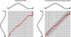 |
Fig. 1 Implementation principles of the DTW algorithm. Left: traditional DTW, with the red dots indicating the optimal alignment path. Right: constrained DTW method, with the Sakoe-Chiba band. The shaded area denotes the constrained region for avoiding pathological alignments. |
2.3 An example
To demonstrate the application of the constrained DTW method in spectral lag analysis, we present a detailed case study of GRB 160530667. The light curves at different energies are shown in the left panel of Fig. 2.
Using the lowest energy band (10-15 keV) as our reference, we systematically shifted this reference light curve relative to each of the eight higher-energy bands. The optimal spectral lag between the reference band and each comparison band was determined by minimizing the constrained DTW distance (see the right panel of Fig. 2). Figure 3 presents the alignment results of the reference light curve with each comparison light curve at its respective optimal time offset. This finding suggests that for GRB 160530667, higher-energy photons generally arrive earlier than lower-energy photons.
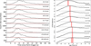 |
Fig. 2 Left: light curves of GRB 160530667 in nine energy bands, with the dashed red lines representing the background fitting curves. Right: scatter plot of DTW distance under different spectral lags. The constrained DTW method is used to select the point with the minimum distance as the optimal result, and the shaded region represents the 1σ uncertainty range. |
3 Comparison with other methods
In this study, we used three methods to measure the spectral lags of the 50 GRBs: the constrained DTW, MCCF methods (e.g., Li et al. 2004; Xiao et al. 2023), and Gaussian peak-time fitting (e.g., Shao et al. 2017). The detailed results obtained with these three methods are listed in Tables A.1, A.2, and A.3.
To evaluate the performance of the constrained DTW method, we systematically compared the Gaussian peak-time fitting and MCCF methods. Figure 4 shows the scatter plots of the spectral lags measured in the 15-22 keV energy band using different method combinations. The scatter plots for the remaining seven energy bands are shown in Fig. A.3. To quantify the overall agreement, we calculated the Spearman rank correlation coefficients for the spectral lags of the 50 GRBs. The average correlation coefficients are 0.81 for Gaussian fitting versus MCCF, 0.78 for Gaussian fitting versus the constrained DTW method, and 0.85 for MCCF versus the constrained DTW method, which indicate strong overall correlation among the three methods.
To provide a more direct comparison among the three methods, we further examined both the distributions of the lag uncertainties and the pairwise normalized lag differences. For a pair of methods i and j, the normalized lag difference is defined as
 (8)
(8)
where τi and τj are the lag estimates from the two methods and σi and σj are their corresponding uncertainties. These quantities together measure the difference between two lag estimates in units of their combined uncertainty. Figure 5 shows the distributions of the lag measurements and their uncertainties for the three methods, while Fig. 6 presents the pairwise distributions of the normalized lag differences. The uncertainties quoted for the mean values and standard deviations of these distributions were estimated using bootstrap resampling of the GRB sample. Overall, the three methods are consistent with each other, with no significant differences found within 3σ. We also note that the DTW uncertainty distribution is, on average, slightly broader than those of the other two methods.
For most bursts, the three methods give broadly consistent results. For instance, GRB 120426090 and GRB 101126198 show good agreement across the different methods. Figures 7 and A.4 show the light curves fitted with two Gaussian fitting schemes. The blue curves represent the peak-focused Gaussian fitting, while the red curves represent the non-peak-focused Gaussian fitting, together with the corresponding spectral-lag results obtained using the four methods.
The Gaussian peak-time fitting method has an intrinsic limitation when applied to asymmetric GRB pulses, because it assumes a symmetric pulse profile. In contrast, a number of asymmetric functions have been proposed in the literature to more realistically describe GRB pulse shapes, including separate exponential functions for the rise and decay phases (Norris et al. 1996), the product of two exponentials (Norris et al. 2005), and the lognormal function (Bhat et al. 2012). Since many GRB pulses exhibit a faster rise and a slower decay, fitting the full pulse with a symmetric Gaussian function can introduce a systematic shift in the inferred peak time and consequently bias the derived spectral lag. This effect is illustrated by GRB 150721242 and GRB 100707032. To demonstrate it, we performed two Gaussian fitting schemes for these two bursts: one focused on the region around the pulse peak and the other using a broader fitting interval without explicitly restricting the fit to the peak region, as shown in Figs. A.5 and A.6. The left panels show the two fitting schemes, while the right panels present the corresponding spectral-lag results obtained with the different methods. When the fitting is restricted to the peak region, the Gaussian-fitting lags become broadly consistent with those derived from the constrained DTW and MCCF methods.
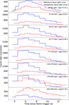 |
Fig. 3 DTW alignment paths between GRB 160530667’s reference energy band and eight comparison bands. The blue curve indicates the light curves of the eight comparison bands, while the red curve indicates the light curve of the reference band under optimal alignment. |
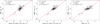 |
Fig. 4 Comparison of spectral lag measurements in the 15-22 keV energy band for 50 GRB samples, employing Gaussian peak-time fitting, the constrained DTW, and MCCF methods. The Spearman rank correlation coefficient r and the corresponding chance probability p are displayed. The comparison results of spectral lag measurements for the remaining seven energy bands are shown in Fig. A.3. |
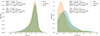 |
Fig. 5 Spectral-lag and uncertainty distributions obtained with the three methods. Left: distributions of the lag measurements derived from DTW, Gaussian fitting, and MCCF. Right: distributions of the corresponding lag uncertainties, which provide a direct comparison of the uncertainties from the three methods. The quoted uncertainties of the mean values and standard deviations are estimated from bootstrap resampling of the GRB sample. |
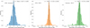 |
Fig. 6 Pairwise distributions of the normalized lag differences among the three spectral-lag estimation methods. For each pair of methods, the normalized lag difference is defined as |

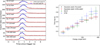 |
Fig. 7 Two Gaussian-fitted light curves of GRB 120426090 and corresponding spectral lag results obtained using four different methods. Left: peak-focused fit (blue curve) and non-peak-focused fit (red curve). |
4 Discussion and conclusion
In this work, we introduced the constrained DTW method as a new approach for measuring spectral lags in GRBs and applied it to a sample of 50 single-pulse Fermi/GBM bursts. We systematically compared the DTW results with those obtained using Gaussian peak-time fitting and MCCF. The spectral lags derived from the constrained DTW method show strong overall correlations with the other two methods, with average Spearman rank correlation coefficients of 0.78 with Gaussian fitting and 0.85 with MCCF. More directly, the distributions of the normalized lag differences show that the three methods are overall consistent with each other, with no significant differences found within 3σ.
Our simulation-based tests further show that, for single-pulse light curves with known input delays and realistic backgrounds, the DTW method can reliably recover the input lag and provides robust uncertainty estimates. These results indicate that the constrained DTW method is a reliable and complementary tool for spectral-lag measurement, rather than a replacement for existing methods.
One advantage of DTW over traditional approaches is that it directly measures the similarity between light curves while naturally enabling moderate local stretching or compression along the time axis. This makes it well suited to cases in which the pulse profiles in different energy bands are similar overall but not strictly related by a simple rigid time shift. At the same time, the method also has limitations. For example, the Sakoe-Chiba band imposes a global path constraint that suppresses pathological alignments. However, if chosen too narrowly it may also restrict alignment flexibility and increase uncertainty. In addition, DTW is computationally more expensive than simpler correlation- or fitting-based methods.
Our comparison with Gaussian peak-time fitting also clarifies an important methodological point. Because GRB pulses are often asymmetric, with a faster rise and a slower decay, fitting the full pulse with a symmetric Gaussian function can bias the inferred peak time and hence, the derived spectral lag. This effect is illustrated by GRB 150721242 and GRB 100707032. When the Gaussian fitting is restricted to the region around the pulse peak, the resulting lag measurements become more consistent with those obtained from DTW and MCCF. In this sense, the present work not only introduces DTW as a new method but also helps clarify the applicability and limitations of existing spectral-lag estimators.
For a large fraction of the bursts in our sample, the spectral lags derived from the constrained DTW method are broadly comparable to those obtained using previously established methods. This indicates that, despite methodological differences, these approaches capture similar overall timing trends in many cases. The overall consistency between DTW and the existing methods also indirectly supports the similarity of pulse morphology across energy bands in many GRBs - for example, in FRED-like pulses. At the same time, the nonnegligible differences seen in some bursts suggest that DTW can reveal aspects of the temporal structure that may not be fully captured by more conventional methods.
We therefore consider the constrained DTW method as a useful additional tool for future studies of more complex light curves, where pulse morphology may evolve significantly across energy bands. It may also be valuable for related applications such as gravitational-lensing searches, where robust comparisons of temporal morphology are particularly important. Beyond GRBs, the constrained DTW framework can in principle, be extended to other astrophysical transients with energy-dependent light curves, such as magnetar bursts and fast radio bursts.
Acknowledgements
We thank the anonymous referee for the constructive suggestions, especially those on the robustness of the DTW method and the treatment of asymmetric pulses in Gaussian fitting. We acknowledge the use of publicly available Fermi/GBM data. This work is supported by Science and Technology Foundation of Guizhou Province (Key Program, No. [2025]021), the National Natural Science Foundation of China (NOs. 12303043 and 12573043), the Guizhou Normal University 2023 Doctoral Research Initiation Project (Project Contract No. GZNUD[2023]), the Natural Science Research Project of the Guizhou Provincial Department of Education ([2024]321), the Guizhou Province Science and Technology Support Program (General Project, No. Qianhe Support [2023] General 333).
References
- Abbott, B. P., Abbott, R., Abbott, T., et al. 2017, ApJ, 848, L13 [CrossRef] [Google Scholar]
- Abdo, A. A., Ackermann, M., Ajello, M., et al. 2009a, Nature, 462, 331 [NASA ADS] [CrossRef] [Google Scholar]
- Abdo, A. A., Ackermann, M., Arimoto, M., et al. 2009b, Science, 323, 1688 [NASA ADS] [CrossRef] [Google Scholar]
- Abraham, S., Mukund, N., Vibhute, A., et al. 2021, MNRAS, 504, 3084 [Google Scholar]
- Acciari, V. A., Ansoldi, S., Antonelli, L. A., et al. 2020, Phys. Rev. Lett., 125, 021301 [Google Scholar]
- Alajlan, N. 2011, J. King Saud University-Computer Inform. Sci., 23, 7 [Google Scholar]
- Berger, E. 2014, ARA&A, 52, 43 [Google Scholar]
- Bernardini, M. G., Ghirlanda, G., Campana, S., et al. 2015, MNRAS, 446, 1129 [Google Scholar]
- Bhat, P. N., Briggs, M. S., Connaughton, V., et al. 2012, ApJ, 744, 141 [NASA ADS] [CrossRef] [Google Scholar]
- Bošnjak, Ž., & Daigne, F. 2014, A&A, 568, A45 [NASA ADS] [CrossRef] [EDP Sciences] [Google Scholar]
- Burgess, J. M., Cameron, E., Svinkin, D., & Greiner, J. 2021, A&A, 654, A26 [NASA ADS] [CrossRef] [EDP Sciences] [Google Scholar]
- Chen, L., Lou, Y.-Q., Wu, M., et al. 2005, ApJ, 619, 983 [Google Scholar]
- Choi, W., Cho, J., Lee, S., & Jung, Y. 2020, IEEE access, 8, 222841 [Google Scholar]
- Dermer, C. D. 2004, ApJ, 614, 284 [NASA ADS] [CrossRef] [Google Scholar]
- Folgado, D., Barandas, M., Matias, R., et al. 2018, Pattern Recog., 81, 268 [Google Scholar]
- Fong, W.-f., Berger, E., & Fox, D. B. 2013, ApJ, 776, 18 [NASA ADS] [CrossRef] [Google Scholar]
- Giao, B. C., & Anh, D. T. 2016, Vietnam J. Comp. Sci., 3, 181 [Google Scholar]
- Golkhou, V. Z., Butler, N. R., & Littlejohns, O. M. 2015, ApJ, 811, 93 [NASA ADS] [CrossRef] [Google Scholar]
- Gompertz, B. P., Ravasio, M. E., Nicholl, M., et al. 2023, Nat. Astron., 7, 67 [Google Scholar]
- Guan, X., Huang, C., Liu, G., Meng, X., & Liu, Q. 2016, Remote Sensing, 8, 19 [Google Scholar]
- Keogh, E., & Ratanamahatana, A. 2004, in 3rd Workshop on Mining Temporal and Sequential Data, in conjunction with 10th ACM SIGKDD Int. Conf. Knowledge Discovery and Data Mining (KDD-2004), Seattle, WA, 1, 1 [Google Scholar]
- Kostelecký, V. A., & Samuel, S. 1989, Phys. Rev. D, 39, 683 [CrossRef] [PubMed] [Google Scholar]
- Lahreche, A., & Boucheham, B. 2021, Expert Systems with Applications, 168, 114374 [Google Scholar]
- Lan, L., Piórkowska-Kurpas, A., Wen, X., et al. 2022, ApJ, 937, 62 [Google Scholar]
- Lee, H.-S. 2019, J. Exercise Rehabilitation, 15, 526 [Google Scholar]
- Leibler, C. N., & Berger, E. 2010, ApJ, 725, 1202 [NASA ADS] [CrossRef] [Google Scholar]
- Li, T.-P., Qu, J.-L., Feng, H., et al. 2004, Chinese J. Astron. Astrophys., 4, 583 [Google Scholar]
- Lu, R.-J., Liang, Y.-F., Lin, D.-B., et al. 2018, ApJ, 865, 153 [NASA ADS] [CrossRef] [Google Scholar]
- MacLachlan, G. A., Shenoy, A., Sonbas, E., et al. 2013, MNRAS, 432, 857 [NASA ADS] [CrossRef] [Google Scholar]
- McBreen, S., Foley, S., Watson, D., et al. 2008, ApJ, 677, L85 [NASA ADS] [CrossRef] [Google Scholar]
- Meegan, C., Lichti, G., Bhat, P. N., et al. 2009, ApJ, 702, 791 [Google Scholar]
- Mei, A., Banerjee, B., Oganesyan, G., et al. 2022, Nature, 612, 236 [NASA ADS] [CrossRef] [Google Scholar]
- Morel, M., Achard, C., Kulpa, R., & Dubuisson, S. 2018, Pattern Recog., 74, 77 [Google Scholar]
- Niennattrakul, V., & Ratanamahatana, C. A. 2009, arXiv e-prints [arXiv:0903.0041] [Google Scholar]
- Norris, J. P., & Bonnell, J. T. 2006, ApJ, 643, 266 [NASA ADS] [CrossRef] [Google Scholar]
- Norris, J. P., Nemiroff, R. J., Bonnell, J. T., et al. 1996, ApJ, 459, 393 [NASA ADS] [CrossRef] [Google Scholar]
- Norris, J., Marani, G., & Bonnell, J. 2000, ApJ, 534, 248 [NASA ADS] [CrossRef] [Google Scholar]
- Norris, J. P., Bonnell, J. T., Kazanas, D., et al. 2005, ApJ, 627, 324 [NASA ADS] [CrossRef] [Google Scholar]
- Ratanamahatana, C. A., & Keogh, E. 2004, in Proceedings of the 2004 SIAM international conference on data mining, SIAM, 11 [Google Scholar]
- Richter, C., & GuÐnason, J. 2023, in ICASSP 2023 - 2023 IEEE International Conference on Acoustics, Speech and Signal Processing (ICASSP), 1 [Google Scholar]
- Sakoe, H., & Chiba, S. 2003, IEEE Trans. Acoustics Speech Signal Process., 26, 43 [Google Scholar]
- Sari, R., & Piran, T. 1997, arXiv e-prints [arXiv:astro-ph/9701002] [Google Scholar]
- Serra, J., & Arcos, J. L. 2012, in Case-Based Reasoning Research and Development - 20th International Conference [Google Scholar]
- Shao, L., Zhang, B. B., Wang, F. R., Dai, Z. G., & Liang, E. W. 2017, ApJ, 844, 126 [Google Scholar]
- Shen, R.-F., Song, L.-M., & Li, Z. 2005, MNRAS, 362, 59 [Google Scholar]
- Strle, B., Mozina, M., & Bratko, I. 2009, in Proceedings of the Workshop on Qualitative Reasoning [Google Scholar]
- Troja, E., Fryer, C., O’Connor, B., et al. 2022, Nature, 612, 228 [NASA ADS] [CrossRef] [Google Scholar]
- Uhm, Z. L., & Zhang, B. 2016, ApJ, 825, 97 [Google Scholar]
- Ukwatta, T., Stamatikos, M., Dhuga, K., et al. 2010, ApJ, 711, 1073 [NASA ADS] [CrossRef] [Google Scholar]
- Ukwatta, T., Dhuga, K., Stamatikos, M., et al. 2012a, MNRAS, 419, 614 [Google Scholar]
- Ukwatta, T. N., Stamatikos, M., Dhuga, K. S., et al. 2012b, ApJ, 711, 1073 [Google Scholar]
- Wei, J.-J., Zhang, B.-B., Shao, L., Wu, X.-F., & Mészáros, P. 2017, ApJ, 834, L13 [Google Scholar]
- Wen, Y., Xiao, S., Jiang, Z.-H., et al. 2026, J. High Energy Astrophys., 53, 100590 [Google Scholar]
- Woosley, S., & Bloom, J. 2006, ARA&A, 44, 507 [NASA ADS] [CrossRef] [Google Scholar]
- Xiao, S., Xiong, S., Zhang, S., et al. 2021, ApJ, 920, 43 [Google Scholar]
- Xiao, S., Xiong, S. L., Wang, Y., et al. 2022, ApJ, 924, L29 [Google Scholar]
- Xiao, S., Tuo, Y. L., Zhang, S. N., et al. 2023, MNRAS, 521, 5308 [Google Scholar]
- Xiao, S., Zhang, Y.-Q., Zhu, Z.-P., et al. 2024, ApJ, 970, 6 [Google Scholar]
- Xiong, S., Wang, C., & Huang, Y. 2023, GRB Coordinates Netw., 33406, 1 [Google Scholar]
- Yang, J., Chand, V., Zhang, B.-B., et al. 2020, ApJ, 899, 106 [NASA ADS] [CrossRef] [Google Scholar]
- Yang, J., Ai, S., Zhang, B.-B., et al. 2022, Nature, 612, 232 [NASA ADS] [CrossRef] [Google Scholar]
- Yu, D., Yu, X., Hu, Q., Liu, J., & Wu, A. 2011, Inf. Sci., 181, 2787 [Google Scholar]
- Zhang, B.-B., Zhang, B., & Castro-Tirado, A. J. 2016, ApJ, 820, L32 [Google Scholar]
- Zhang, Z., Tavenard, R., Bailly, A., et al. 2017, Inf. Sci., 393, 91 [Google Scholar]
- Zhao, J., & Itti, L. 2018, Pattern Recog., 74, 171 [Google Scholar]
Appendix A Simulation-based validation of the DTW method
To assess the possible bias and uncertainty calibration of the DTW method, we performed simulations using single-pulse GRB light curves with a known input time delay. Following the approach of Wen et al. (2026), we used the pyipn simulation package (Burgess et al. 2021) to generate theoretical single-pulse light curves based on the Norris pulse profile (Norris et al. 1996; Norris et al. 2005), which has a Fast Rise and Exponential Decay (FRED) shape. The pulse model is given by
![Mathematical equation: \begin{split} F(t)=K \cdot \exp\left(2\sqrt{\frac{\tau_{\rm rise}}{\tau_{\rm decay}}}\right) \cdot \exp\left[-\frac{\tau_{\rm rise}}{t-t_{\rm start}}-\frac{t-t_{\rm start}}{\tau_{\rm decay}}\right], \end{split}](/articles/aa/full_html/2026/06/aa58655-25/aa58655-25-eq10.png) (A.1)
(A.1)
where K is the pulse amplitude, tstart is the pulse start time, and τrise and τdecay characterize the temporal evolution of the pulse. In our simulations, we set K = 100,000 counts s−1, τrise = 0.1 s, and τdecay = 0.02 s. We generated pairs of light curves with tstart,1 = 1.0 s and tstart,2 = 1.32 s, corresponding to a groundtruth delay of ∆ttrue = 0.32 s. A constant background was added to both light curves before Poisson sampling. One example of the resulting simulated light curve, including both background and counting-statistics fluctuations, is shown in Fig. A.1.
Based on this setup, we performed Nsim = 500 independent realizations to evaluate the statistical reliability of the DTW-derived confidence regions. For each nominal confidence level, we computed the empirical coverage frequency, p = M/Nsim, where M is the number of realizations for which the corresponding confidence region contains the true delay of ∆ttrue = 0.32 s. The relation between the nominal confidence level and the empirical coverage is shown in Fig. A.2. We find that the empirical coverage is overall consistent with the identity relation, indicating that the DTW uncertainty estimates are robust. Within this simulation setup, we do not find evidence for a significant systematic bias in the recovered time lags.
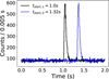 |
Fig. A.1 Example of a simulated single-pulse GRB light curve generated from the Norris pulse profile, including a constant background and Poisson counting fluctuations. |
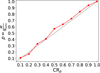 |
Fig. A.2 Reliability diagram for the DTW-derived time-delay confidence regions based on Nsim = 500 simulations. The nominal confidence level is compared with the empirical fraction of trials in which the true delay (∆ttrue = 0.32 s) is contained within the corresponding confidence region. The black dotted line indicates the ideal identity relation. The overall agreement between the two demonstrates the robustness of the DTW uncertainty estimates. |
The DTW-derived spectral lags (s) for the sample of 50 GRBs detected by GBM. The lowest energy band (10 – 15 keV) serves as the reference.
The MCCF-derived spectral lags (s) for the sample of 50 GRBs detected by GBM. The lowest energy band (10 – 15 keV) serves as the reference.
The Gaussian Peak-Time-derived spectral lags (s) for the sample of 50 GRBs detected by GBM. The lowest energy band (10 – 15 keV) serves as the reference.
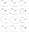 |
Fig. A.3 Comparison of spectral lag measurements across the remaining seven energy bands for 50 GRB samples, employing Gaussian Peak-Time fitting, the constrained DTW, and MCCF methods. The Spearman rank correlation coefficient r and the corresponding chance probability p are displayed. |
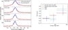 |
Fig. A.4 Similar to Fig. 7, but for GRB 101126198. To improve the signal-to-noise ratio and enhance the statistical significance of the lag measurement, the original energy bands are merged into four broader channels. |
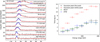 |
Fig. A.5 Two Gaussian-fitted light curves of GRB 150721242 and the corresponding spectral lag results obtained using four different methods. In the left panel, the blue curve represents the peak-focused fitting, while the red curve represents the non-peak-focused fitting. |
All Tables
The DTW-derived spectral lags (s) for the sample of 50 GRBs detected by GBM. The lowest energy band (10 – 15 keV) serves as the reference.
The MCCF-derived spectral lags (s) for the sample of 50 GRBs detected by GBM. The lowest energy band (10 – 15 keV) serves as the reference.
The Gaussian Peak-Time-derived spectral lags (s) for the sample of 50 GRBs detected by GBM. The lowest energy band (10 – 15 keV) serves as the reference.
All Figures
|
Fig. 1 Implementation principles of the DTW algorithm. Left: traditional DTW, with the red dots indicating the optimal alignment path. Right: constrained DTW method, with the Sakoe-Chiba band. The shaded area denotes the constrained region for avoiding pathological alignments. |
| In the text | |
|
Fig. 2 Left: light curves of GRB 160530667 in nine energy bands, with the dashed red lines representing the background fitting curves. Right: scatter plot of DTW distance under different spectral lags. The constrained DTW method is used to select the point with the minimum distance as the optimal result, and the shaded region represents the 1σ uncertainty range. |
| In the text | |
|
Fig. 3 DTW alignment paths between GRB 160530667’s reference energy band and eight comparison bands. The blue curve indicates the light curves of the eight comparison bands, while the red curve indicates the light curve of the reference band under optimal alignment. |
| In the text | |
|
Fig. 4 Comparison of spectral lag measurements in the 15-22 keV energy band for 50 GRB samples, employing Gaussian peak-time fitting, the constrained DTW, and MCCF methods. The Spearman rank correlation coefficient r and the corresponding chance probability p are displayed. The comparison results of spectral lag measurements for the remaining seven energy bands are shown in Fig. A.3. |
| In the text | |
|
Fig. 5 Spectral-lag and uncertainty distributions obtained with the three methods. Left: distributions of the lag measurements derived from DTW, Gaussian fitting, and MCCF. Right: distributions of the corresponding lag uncertainties, which provide a direct comparison of the uncertainties from the three methods. The quoted uncertainties of the mean values and standard deviations are estimated from bootstrap resampling of the GRB sample. |
| In the text | |
|
Fig. 6 Pairwise distributions of the normalized lag differences among the three spectral-lag estimation methods. For each pair of methods, the normalized lag difference is defined as |
| In the text | |
|
Fig. 7 Two Gaussian-fitted light curves of GRB 120426090 and corresponding spectral lag results obtained using four different methods. Left: peak-focused fit (blue curve) and non-peak-focused fit (red curve). |
| In the text | |
|
Fig. A.1 Example of a simulated single-pulse GRB light curve generated from the Norris pulse profile, including a constant background and Poisson counting fluctuations. |
| In the text | |
|
Fig. A.2 Reliability diagram for the DTW-derived time-delay confidence regions based on Nsim = 500 simulations. The nominal confidence level is compared with the empirical fraction of trials in which the true delay (∆ttrue = 0.32 s) is contained within the corresponding confidence region. The black dotted line indicates the ideal identity relation. The overall agreement between the two demonstrates the robustness of the DTW uncertainty estimates. |
| In the text | |
|
Fig. A.3 Comparison of spectral lag measurements across the remaining seven energy bands for 50 GRB samples, employing Gaussian Peak-Time fitting, the constrained DTW, and MCCF methods. The Spearman rank correlation coefficient r and the corresponding chance probability p are displayed. |
| In the text | |
|
Fig. A.4 Similar to Fig. 7, but for GRB 101126198. To improve the signal-to-noise ratio and enhance the statistical significance of the lag measurement, the original energy bands are merged into four broader channels. |
| In the text | |
|
Fig. A.5 Two Gaussian-fitted light curves of GRB 150721242 and the corresponding spectral lag results obtained using four different methods. In the left panel, the blue curve represents the peak-focused fitting, while the red curve represents the non-peak-focused fitting. |
| In the text | |
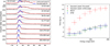 |
Fig. A.6 Similar to Fig. A.5 but for GRB 100707032. |
| In the text | |
Current usage metrics show cumulative count of Article Views (full-text article views including HTML views, PDF and ePub downloads, according to the available data) and Abstracts Views on Vision4Press platform.
Data correspond to usage on the plateform after 2015. The current usage metrics is available 48-96 hours after online publication and is updated daily on week days.
Initial download of the metrics may take a while.