


| Issue |
A&A
Volume 710, June 2026
|
|
|---|---|---|
| Article Number | A295 | |
| Number of page(s) | 17 | |
| Section | Extragalactic astronomy | |
| DOI | https://doi.org/10.1051/0004-6361/202558621 | |
| Published online | 23 June 2026 | |
Supermassive Black Hole Winds in X-rays: SUBWAYS
IV. Tracing radio emission and unveiling the role of winds
1
Dipartimento di Fisica e Astronomia, Università di Bologna, Via P. Gobetti 93/2, 40129 Bologna, Italy
2
INAF – Istituto di Radioastronomia, Via P. Gobetti 101, 40129 Bologna, Italy
3
INAF – Istituto di Astrofisica e Planetologia Spaziali, Via Fosso del Cavaliere, 00133 Roma, Italy
4
INAF – Osservatorio di Astrofisica e Scienza dello Spazio di Bologna, Via Gobetti, 93/3, 40129 Bologna, Italy
5
ASTRON, the Netherlands Institute for Radio Astronomy, Postbus 2, 7990 AA, Dwingeloo, The Netherlands
6
Kapteyn Astronomical Institute, University of Groningen, P.O. Box 800, 9700 AV, Groningen, The Netherlands
7
Department of Physics, Technion, Haifa 32000, Israel
8
Physics Department, Tor Vergata University of Rome, Via della Ricerca Scientifica 1, 00133 Rome, Italy
9
INAF – Astronomical Observatory of Rome, Via Frascati 33, 00040 Monte Porzio Catone, Italy
10
INFN – Rome Tor Vergata, Via della Ricerca Scientifica 1, 00133 Rome, Italy
11
Dipartimento di Matematica e Fisica Università degli Studi Roma Tre, Via della Vasca Navale 84, 00146 Rome, Italy
12
Department of Physics and Astronomy, College of Charleston, Charleston, SC 29424, USA
13
INAF – Osservatorio Astrofisco di Arcetri, Largo E. Fermi 5, 50127 Firenze, Italy
14
Departament de Física, EEBE, Universitat Politécnica de Catalunya, Av. Eduard Maristany 16, S-08019 Barcelona, Spain
15
INAF – Osservatorio Astronomico di Trieste, Via G.B. Tiepolo 11, 34143 Trieste, Italy
16
Department of Physics, Informatics and Mathematics, University of Modena and Reggio Emilia, 41125 Modena, Italy
17
Department of Physics and Astronomy, Clemson University, Kinard Lab of Physics, Clemson, SC 29634, USA
18
Department of Physics, Institute for Astrophysics and Computational Sciences, The Catholic University of America, Washington, DC 20064, USA
19
Space Telescope Science Institute, 3700 San Martin Drive, Baltimore, MD 21218, USA
20
Instituto de Astronomía, Universidad Nacional Autónoma de México, Circuito Exterior, Ciudad Universitaria, Ciudad de México, 04510, México
21
Department of Astronomy, University of Michigan, 1085 South University Avenue, Ann Arbor, MI 48109, USA
22
Centro de Astrobiología (CAB), CSIC–INTA, Cra. de Ajalvir Km. 4, 28850 Torrejón de Ardoz, Madrid, Spain
23
Univ. Grenoble Alpes, CNRS, IPAG, 38000 Grenoble, France
24
INAF – Osservatorio Astronomico di Brera, Via Bianchi 46, 23807 Merate (LC), Italy
25
Max-Planck-Institut für extraterrestrische Physik (MPE), Gießenbachstraße 1, D-85748 Garching bei München, Germany
26
Como Lake Center for Astrophysics (CLAP), DiSAT, Università degli Studi dell’Insubria, Via Valleggio 11, 22100 Como, Italy
★ Corresponding author: This email address is being protected from spambots. You need JavaScript enabled to view it.
Received:
17
December
2025
Accepted:
29
April
2026
Abstract
Context. Most active galactic nuclei (AGNs) are radio quiet (RQ), with radio emission that may arise from star-formation activity, AGN-driven winds, weak jets, and coronal activity. Disentangling these mechanisms is challenging and requires detailed multi-wavelength investigations, but it is crucial for quantifying AGN feedback in galaxy evolution.
Aims. We present a detailed radio investigation of 22 X-ray-selected AGNs in the Supermassive Black Hole Winds in X-Rays (SUBWAYS) sample (Lbol ≃ 1044.9 − 46.3 erg/s, z = 0.1–0.5), selected to systematically search for ultra-fast outflows (UFOs). The UFOs are detected in ∼30% of the targets, with measured velocities and kinetic luminosities, making the sample particularly well-suited for investigating the role and signatures of multi-scale outflows at different frequencies.
Methods. We built the radio spectral energy distribution of the sources complementing our proprietary data, collected with the JVLA at 1.5 and 6 GHz, with images from LoTSS (145 MHz) and other publicly available radio surveys between 150 and 1400 MHz. We investigated the role and occurrence of the aforementioned mechanisms, with particular interest in outflows and their possible relation to UFOs. To achieve this, we combined information on spectral indices, luminosities, and morphologies of radio emission with properties derived in other wavebands, such as the star formation rate, the X-ray luminosity, the Eddington ratio, or the UFO kinetic luminosity.
Results. All sources are detected and are mostly consistent with RQ AGNs. For ∼80% of the sources, the data suggest the presence of an outflow (wind or weak jet). Interestingly, our results indicate that AGNs with UFOs tend to have larger radio extension and a steep radio spectrum consistent with outflows. Moreover, the radio emission of the six UFO hosts is consistent with predictions from wind-driven shock models, possibly indicating a direct connection between the two phases. Alternatively, this may simply reflect physical conditions that favour the production of both phenomena.
Key words: instrumentation: interferometers / methods: observational / ISM: jets and outflows / galaxies: active / galaxies: evolution / radio continuum: galaxies
© The Authors 2026
 Open Access article, published by EDP Sciences, under the terms of the Creative Commons Attribution License (https://creativecommons.org/licenses/by/4.0), which permits unrestricted use, distribution, and reproduction in any medium, provided the original work is properly cited.
This article is published in open access under the Subscribe to Open model. This email address is being protected from spambots. You need JavaScript enabled to view it. to support open access publication.
1. Introduction
Accretion onto supermassive black holes (SMBHs) can light up the nuclear regions of galaxies, giving rise to the so-called active galactic nuclei (AGNs), which are among the most energetic objects in the Universe (see Kormendy & Ho 2013 and Alexander et al. 2025 for reviews). Active galactic nuclei have been shown to inject significant amounts of energy and momentum into their surroundings from parsec to Mpc scales. This occurs via multiple channels, including direct radiation (e.g. Ciotti et al. 2010), jets of relativistic plasma (e.g. Fabian 2012), and massive multi-phase gas winds (e.g. Crenshaw et al. 2003). In particular, through the interaction with the interstellar medium (ISM), powerful AGN-driven outflows, in the form of winds or jets, have proven to be capable of reproducing the scaling relations between SMBH mass and galaxy properties (Cattaneo et al. 1999; Kauffmann & Haehnelt 2000; King & Pounds 2015; King et al. 2005; Gaspari et al. 2020; King & Pounds 2015; Fabian 2012). While synchrotron emission from powerful relativistic jets dominates the radio luminosity only in a minority of AGNs, classified as radio loud (RL, L6 GHz = 1023 − 27 W/Hz), the majority falls into the radio quiet (RQ; L6 GHz = 1021 − 23 W/Hz) category, where the origin of radio emission is still debated. In RQ AGNs, radio emission can arise from a plethora of processes, possibly overlapping, including AGN-driven winds, weak jets, coronal activity, and star-formation activity (see Padovani 2017; Panessa et al. 2019 for extensive reviews). Disentangling these mechanisms and understanding how the energy they release couples with the ISM is challenging and requires detailed spectral and morphological analysis. However, obtaining observational constraints is crucial for modelling AGN feedback and galaxy evolution.
The AGN-driven winds are indeed detected in any gas phase, at different ionisation states, velocities, and distances from the inner SMBH. These range from sub-relativistic (0.1 − 0.25 c), highly ionised, ultra-fast outflows (UFOs), arising at few gravitational radii (e.g. Chartas et al. 2002; Tombesi et al. 2010; Pounds 2014; Tombesi et al. 2015; Matzeu et al. 2023; Gianolli et al. 2024), down to the slower (∼500 − 2000 km/s) outflows detected on kpc scales, in the atomic and molecular gas phases (e.g. Zakamska & Greene 2014; Morganti et al. 2016, and see Cicone et al. 2018 for a review). In luminous RQ AGNs, it has been proposed that the shocks generated by radiatively driven winds can accelerate electrons, producing synchrotron radio emission on scales larger than 100 pc with νLν ∼ 10−5 LAGN (Zakamska & Greene 2014; Nims et al. 2015). However, how the different wind phases are connected to each other is still poorly understood.
Recent observations also showed that low-luminosity (log P1.4 GHz < 1024 W/Hz) galaxy-scale radio jets, which are much more common than their high-power counterparts (Mauch & Sadler 2007, Sabater et al. 2019; Venturi et al. 2021; Speranza et al. 2022; Murthy et al. 2022; Cresci et al. 2023; Ulivi et al. 2024), remain trapped in the ISM for longer, affecting the surrounding medium over a large volume (e.g. Bicknell 1994; Jarvis et al. 2019; Mukherjee 2025). Such low-power jets can still account for the radio emission observed in RQ AGNs. However, AGN winds and jets can coexist (e.g. Tombesi et al. 2012; Mestici et al. 2024), making it complicated to understand their potential causal connection. In addition, recent work discusses the possibility that UFOs can accelerate ultra-high-energy cosmic rays. If such associations are confirmed, they would provide further motivation to test whether X-ray UFOs correlate with extended non-thermal radio emission (Karwin et al. 2023; Ehlert et al. 2025).
The current literature providing a detailed investigation of the radio emission in UFO hosts has been largely limited to single-object analyses or archival studies (e. g. Falcke et al. 1998; Tombesi et al. 2010, Tombesi et al. 2012, 2014; Morganti 2017; Giroletti et al. 2017; Wang et al. 2021; Longinotti et al. 2023; Maksym et al. 2023; Zanchettin et al. 2023; Yamada et al. 2024b).
In this paper we present the analysis of new Jansky Very Large Array (JVLA) observations, obtained at 1.5 and 6 GHz of 22 quasars belonging to the Supermassive Black Holes Winds in X-rays (SUBWAYS) sample. By combining JVLA data with radio observations from additional surveys, together with the wealth of multi-wavelength data available for the SUBWAYS sample, we investigate the origin of the radio emission (star formation, coronae, or outflows) and characterise the contribution of AGN-driven outflows1, with particular emphasis on UFO hosts. This work constitutes the first systematic analysis that exploits dedicated follow-up observations for a sample of RQ AGNs with detected UFOs.
This paper is organised as follows: in Sect. 2 and 3 we describe the sample and how the data have been collected and reduced; in Sect. 4 and 5 we discuss the results and consider the potential origins of the radio emission, investigating how the radio properties of the sample relate to those derived in other wavebands. In Sect. 6 we draw our conclusions.
Throughout this work, a standard Lambda cold dark matter (ΛCDM) cosmology has been adopted, with H0 = 71 kms−1 Mpc−1, ΩΛ = 0.73, and Ωm = 0.27. The uncertainties are always reported at 1σ.
2. The sample
SUBWAYS was born with the aim of increasing the number of known UFO hosts with multi-wavelength observations. The whole project is based on a large XMM-Newton campaign (∼1.5 Ms of observing time in 2019–2020; Brusa et al. 2022) of a sample of 17 (plus five collected from the XMM archive with comparable spectral quality) X-ray selected AGNs (mostly Type 1 quasar (QSO), with log(MBH/M⊙) = 7.46 − 9.22 and −1.92 < log λEdd < 0.35), chosen at redshift z = 0.1–0.5 and with bolometric luminosity Lbol ≃ 1044.9 − 46.3 erg/s. In Table 1 we list the 22 sources belonging to SUBWAYS with their basic properties. Sources with a UFO detection in the confidence interval ≥99% are placed above the horizontal line. The unprecedented quality reached by XMM-Newton spectra allowed a detailed investigation of under-explored ranges of redshift and luminosity in UFO studies. From the main analysis of the XMM-Newton observations, Matzeu et al. (2023, Paper I) reported, in seven of the 22 AGNs (∼30%), significant detection of absorption lines corresponding to high column density, highly ionised iron with outflow velocities in the range −0.3 ≤ vout/c ≤ −0.05, consistent with the expectations for UFOs. Complementary UV imaging data have been obtained with Hubble Space Telescope (HST; PI: G. Kriss), but no counterpart for the UFO was found (Mehdipour et al. 2023, Paper II). These results could be attributed either to an excessively high ionisation state or to a low covering fraction of the UV-emitting source. Moreover, correlations of SUBWAYS UFO parameters with X-ray luminosity are found to be much stronger than those with the UV luminosity (Gianolli et al. 2024, Paper III), suggesting that the innermost regions of the AGNs are more significantly involved than the accretion disk in powering sub-relativistic winds. In fact, though for four objects with UFO detection thermal pressure could in theory launch the outflow, it cannot explain the outflow velocity of UFOs, suggesting that a combination of magnetically and radiatively driven processes is needed (see Fig. 11b of Paper II).
General parameters of the sources in the SUBWAYS sample.
Figure 1 shows the bolometric luminosity (Lbol) redshift plane of the SUBWAYS sample in the context of literature samples of detected X-ray outflows: the one compiled by Yamada et al. (2024a, Y24), which includes 132 AGNs at z = 0–4, and encompasses 93 UFO hosts known so far (including the SUBWAYS sample) and the one from Tombesi et al. (2010, T10, included in Y24 as well), which represents the low-redshift (z ≤ 0.1) comparison sample used in Paper III and, for consistency, also adopted in this work. The red and purple contours instead show the location in the Lbol − z plane of the samples of Laor & Behar (2008) and Panessa & Giroletti (2013), which we chose as a comparison for the study of the correlation of X-ray and radio luminosity.
 |
Fig. 1. Bolometric luminosity as a function of redshift. The grey contours highlight the AGNs of Yamada et al. (2024a, Y24), the red ones are the data from Laor & Behar (2008, LB08), and those in purple the data from Panessa & Giroletti (2013, PG13). We choose LB08 and PG13 as a comparison for the study of the X-ray-radio luminosity correlation. Then we plot the objects in the SUBWAYS sample (blue empty dots) and a comparison sample from Tombesi et al. (2010, T10, black empty diamonds). UFO hosts are marked by stars and triangles in SUBWAYS and T10 respectively. |
3. Data
3.1. JVLA data reduction
We made dedicated observations of the sample with the JVLA interferometer between August 2020, May 2023 (PI: F. Panessa), and January 2026 (PI: E. Amenta) in B configuration (bmin ∼ 0.21 km, bmax ∼ 11.1 km). This set-up has, for the purposes of this work, the right trade-off in terms of maximum and minimum baseline length, providing indeed both good resolution and good sensitivity, necessary for a meaningful morphological analysis.
The data were collected using the L- and C-band receivers (1.5 and 6 GHz respectively), with 30 minute and 5 minute observations of each target, respectively. Taking into account a 50% overhead for each observing block, which includes telescope initial set-up, phase and amplitude calibration, and slewing between sources, the total observing time is equal to 18.5 observing hours in the L band and 2.88 in the C band. The predicted resolution is 4.3″ at 1.5 GHz and 1″ at 6 GHz, with 1″ being ∼2 − 4 kpc at the redshift of our sources.
For all observing blocks, we downloaded the datasets calibrated by the observatory pipeline2, then checked the goodness of automatic calibration and, if necessary, improved target flagging with AOFlagger3 (Offringa 2010).
The imaging was performed with the Common Astronomy Software Applications package (The CASA Team 2022 CASA 6.6.3.22 version4) task tclean, weighting the visibilities with the Briggs scheme (Briggs 1995), with weighting parameter as listed in Table A.1. We based the flux-density scale on measurements of VLA primary amplitude calibrators by Perley & Butler (2013). Whenever the noise displayed a non-uniform pattern, before attempting the self-calibration, we tried imaging the data with w-stacking clean (WSClean)5 (Offringa et al. 2014) and this often improved the results. The images produced with this software are labelled* in Table A.1. This was not sufficient for two of the targets, PG1425+267 and HB891529+050, for which we performed one round of phase self-calibration within CASA.
All parameters relative to the final images are listed in Table A.1. The typical resolutions are  and θ6 GHz ∼ 1″, with a median noise equal to σrms = 0.02 mJy beam−1 and 0.012 mJy beam−1 at 1.5 and 6 GHz respectively.
3.2. Complementary data
To investigate the morphology of the sources at different frequencies and their broadband radio spectral shape, we combined the aforementioned JVLA 1.5 and 6 GHz simultaneous data with the LOw Frequency ARray Two-metre Sky Survey (LoTSS; Shimwell et al. 2017, 2022) data. The aim of LoTSS is to survey the whole northern sky at 145 MHz with a resolution of ∼6″, comparable to that of the proprietary data, and a sensitivity ∼0.10 mJy beam−1. There are LoTSS mosaics available for 18 of 22 targets (the remaining four are too far south to be observed with LOFAR); in particular, 11 of the mosaics are currently released within the LoTSS collaboration in DR3 (Shimwell et al. 2026).
To further sample the 145 MHz-6 GHz frequency range and test temporal variability, we also considered images from other surveys, which we list here together with their main properties:
– TGSS (TIFR Giant Metrewave Radio Telescope) at about 150 MHz (ADR1; Intema et al. 2017)6 with a 2″ resolution and a median noise of 3.5 mJy beam−1 (Intema et al. 2017). We rely on TGSS for the four sources located too far south to fall into the LoTSS footprint.
– RACS – low Data Release 1 (Rapid ASKAP Continuum Survey DR1) images at 888 MHz have a common resolution of 25″, with a uniform sensitivity of about 0.25 mJy beam−1 (McConnell et al. 2020; Hale et al. 2021). The RACS cutouts are available for 15 targets.
– FIRST (Faint Images of the Radio Sky at Twenty-cm) Survey is a survey done with VLA in B configuration at 1.4 GHz, with a 5″ resolution and median noise of 0.15 mJy beam−1 (Becker et al. 1995). Among the objects belonging to the SUBWAYS sample, four are not covered by FIRST.
– VLASS (Very Large Array Sky Survey) is conducted by the VLA in B configuration, with multi-epoch observations at 3 GHz, separated by approximately 32 months. Observations are available for three epochs, with a sensitivity ∼0.16 mJy beam−1 and a resolution ∼2.4″ (Lacy et al. 2016, 2020; Gordon et al. 2021). Cutouts of the three epochs are available for all objects, but, unless otherwise specified, we refer only to the third because it is the most recent one.
A more in-depth discussion of the use of these data can be found in the following section. The final images are displayed in Appendix B with L-band white contours superimposed on the C-band colours. The green contours belong to the LoTSS images.
4. Results
4.1. Detection rates and morphologies
All sources (22/22, 100%) are detected at 1.5 and 6 GHz, and 17/18 (∼94%) are detected at 150 MHz. Due to the worse resolution and/or sensitivity, in the remaining complementary data the fraction of detected objects decreases resulting in 11/15 (∼73%), 13/18 (∼72%) and 13/22 (∼59%) at 888 MHz, 1.4, and 3 GHz, respectively. This shows the importance and need for dedicated observations for such faint objects.
A compact emitting region, spatially coincident with the optical centre of the AGN, is detected for all of the sources at both 1.5 and 6 GHz, with a signal-to-noise ratio larger or equal to 6 in all cases (see Appendix A). An exception is the 1.5 GHz image of PG1352+183, where the emission is detected at 3σrms only (see Appendix B). For the four targets not covered by LoTSS we derive upper limits from TGSS (Col. 3 of Table 3, more comments in Sect. 4.5).
We provide a morphological classification of the sources by comparing the highest (6 GHz) frequency proprietary images and the lowest (145 MHz) frequency LoTSS one, which may be sensitive to different components. To do so, for individual components, we fit a Gaussian within the 3σrms contours in CASAviewer at both frequencies. A deconvolved value is given by gaussfit, to which the algorithm already associated uncertainty. If the source is found to be resolved, this approach provides the least instrumentally biased measurements, which is important for compact emitting regions, as in the case (of the majority) of this sample.
With this approach 11/22 (50%) sources are classified as unresolved at all frequencies. In these cases, we associate with their extension an upper limit given by the major axis of the restoring beam. Only one source (PG1427+480), appears to be unresolved at 1.5 GHz (L band) and 6 GHz (C band), but shows extensions at 150 MHz, thus we classify it overall as resolved (Fig. 3). Moreover, at a distance ∼1.4′ in the north-east direction of PG1427+480, some very faint extended emission is detected in the LoTSS image. In Fig. 3 we plot in green the contours of the low resolution LoTSS image (20 × 20″) where the detection of such features reaches 9σrms. There is no clear morphological connection with the target nuclear emission, and overlays with the optical/IR surveys reveal some background objects in the same region. However, there is no clear optical/IR identification, leaving open the possibility that the emission is associated with PG1427+480.
 |
Fig. 2. Images of the ‘multi-component’ sources. Colours at 6 GHz with σrms ⋅ [ − 3, 3, 6, 12, 24, 48, 96] contours at 1.5 GHz (white) and 145 MHz (green). The beams are shown in the bottom-left corner of each panel. Labels A, B, and C mark distinct radio components: A denotes the nuclear (core) component spatially coincident with the optical AGN position, while B and C denote spatially-separated extranuclear components (i.e. features that are not coincident with the optical/IR nucleus and that extend beyond the host’s optical light profile) likely related to AGN outflows. |
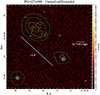 |
Fig. 3. Image of PG1427+480, showing the extended emission detected in the north-east direction of the target, which is located in the lower-right region of the image. Colours at 6 GHz with σrms ⋅ [ − 3, 3, 6, 12, 24, 48, 96] contours at 1.5 GHz (white) and 145 MHz (6″in green, 20″in cyan). The beams are shown in the bottom-left corner of the panel. The black cross marks the optical position of the AGN. |
All objects with an angular size larger than the beam major axis are resolved and classified as extended. In all the targets that belong to this class, the compact central emitting source is surrounded by extended emission. Among these, three sources (PG0804+761, 2MASXJ1653+23, and PG1425+267) exhibit multiple components (Fig. 2), where some features are well distinguished from the compact central structure, unambiguously extended for several arcseconds, and are not associated with neighbouring sources (see also Appendix B). We measure the maximum extension of these three targets with the ruler tool in CASAviewer, taking as a reference the 3σrms contours.
At both 1.5 and 6 GHz 10/22 (∼45%) targets belong to the class of extended sources, with three of them being multi-components (∼14% of the total sample). In LoTSS images 11 objects are resolved with the same number (3) of multi-components seen by JVLA. The results are summarised in Table 2.
Morphologies and sizes of the targets from JVLA (6 GHz) and LoTSS images.
We also note that there are two targets that show adjacent radio emission, namely PG0947+396 and PG0953+414 (see Appendix B). However, further multi-wavelength investigation reveals that the emission is unrelated to the targets but is instead associated with an edge-on spiral galaxy in the first case, and a blazar, SDSSJ095651+411558 at z ∼ 0.6, in the second.
4.2. Flux densities
For unresolved sources, we extracted the integrated flux densities within the 3σrms contours from the images at their original resolution, at all frequencies, using the task imstat.
For extended sources instead, we first match the image resolution of the proprietary data to derive consistent measurements that can be used to compute spectral indices reliably between 145 MHz and 1.5 GHz and between 1.5 and 6 GHz. We note that all sources, even when resolved, except for PG1425+267, have sizes smaller than the largest C-band angular scale recoverable by the instrument (29″), ensuring no flux loss. Hence, only for PG1425+267 we set a cut in baseline length during imaging (bmin ∼ 2585λ), so that all data are sensitive to the same scales of emission at both frequencies (see Table A.1).
For all the extended targets, we first created new images at 6 GHz with a natural weighting, then smoothed the outcomes with the task imsmooth to match the beam at 1.5 GHz. The final images at 6 GHz have θ6 GHz ∼ 4″ − 5″, for the targets labelled with † in Table A.1. The flux densities are then measured from these images following the 3σrms contours. The same approach is used to extract flux densities from complementary surveys. We note that the resolution of the archival images from FIRST and VLASS is similar enough to LoTSS and the proprietary data to allow for a qualitative comparison. Lastly, despite the much worse resolution, RACS data can be useful in reconstructing the overall SED (spectral energy distribution) shape. Further discussion on this can be found in Sect. 4.5.
The uncertainty associated with the integrated flux density Fν is computed as
 (1)
(1)
where δFν is the fraction of uncertainty associated with the flux density calibration, dependent on instrument and frequency, ⟨σrms⟩ν is the average noise at frequency ν, and nbeams the area encompassed by the source in the beam unit. We used the standard JVLA flux density scale calibration uncertainty (5%) for the proprietary data, FIRST and VLASS, while for LoTSS images we used the standard flux density calibration uncertainty for the DR2 δFν = 15%. For RACS images we assumed a flux density scale calibration uncertainty of 5%. All measurements are reported in Table 3. The tabulated VLASS flux density is measured from the third and most recent epoch.
Integrated flux densities used in this work and their associated uncertainties.
To compute the σFν of unresolved objects, nbeams is equal to unity, while in all the other cases it is the area used for measurement in units of beam. Whenever the target is undetected upper limits are derived as 3σrms.
4.3. Spectral indices
To study the radio spectral shape, we computed the slopes of the spectra between 145 MHz and 1.5 GHz ( ) and between 1.5 and 6 GHz (
 ).
).
The spectral index is computed as
 (2)
(2)
with associated uncertainty
 (3)
(3)
where ν1 and ν2 are, respectively, the lower and higher frequency between which the spectral slope is computed.
In the left panel of Fig. 4, we show the distribution of the spectral index; more specifically, the filled histogram represents the distribution of the values computed between 1.5 and 6 GHz, while the barred one represents the distribution between 145 MHz and 1.5 GHz. The upper limits are shown in grey. We note that the values of  derive from simultaneous observations, thus they constitute a robust view of the spectral slope at those frequencies, avoiding potential artificial steepening and/or flattening due to strong variability.
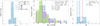 |
Fig. 4. Left: Spectral index distribution of the sample. The filled histogram represents the values computed between 1.5 and 6 GHz, while the barred one those computed between 145 MHz and 1.5 GHz. Middle: Histogram comparing the total radio luminosities of the sample. Blue: 145 MHz. Violet: 1.5 GHz. Green: 6 GHz. The upper limits at 145 MHz have been excluded. Right: Radio loudness parameter distribution of the sample. The convention followed is RX = log (LR(6 cm)/LX(2 − 10 KeV)) (Terashima & Wilson 2003). The filled histogram represents the values of RX computed for the UFO hosts, and the barred histogram those derived for the non-UFO hosts. The vertical red line marks the –4.5 limit set by Terashima & Wilson (2003). RQ AGNs tend to dominate the sample, while RL AGNs represent only a small fraction, specifically 6/21 with the original limit RX = –4.5. |
The spectral index of the nuclear and extranuclear components of 2MASXJ1653+23 and PG0804+761 are reported separately in Table 4. Overall the spectral index distributions span from 0.15 up to 0.68 at lower frequencies, and from –0.17 up to 0.99 at higher ones, with median values 0.57 ± 0.05 and 0.45 ± 0.08 for  and
and  respectively, computed taking into account the upper limits through a Kaplan-Maier (KM) survival analysis7.
Spectral indices and radio luminosities of the targets.
4.4. Radio luminosities and radio loudness
We calculate the characteristic monochromatic radio powers at 145 MHz, 1.5, and 6 GHz, using the following expression
 (4)
(4)
where Fν is the flux density, DL the luminosity distance at redshift z (see Table 1), and αR the radio spectral index, which is substituted with  when computing L145 MHz, while
  is preferred for estimating both L1.5 GHz and L6 GHz. An uncertainty is associated according to the following
 (5)
(5)
The values are reported in Table 4 and shown in the histograms in the middle panel of Fig. 4. The characteristic spectral luminosities range between 22.60 < log L145 MHz < 27.06 W/Hz at the lowest frequency, and between 21.63 < log L6 GHz < 25.51 W/Hz at the highest, with median values 23.28, 22.70, 22.43 W/Hz at 145 MHz, 1.5 GHz, and 6 GHz, respectively.
In addition, taking into account the entire radio emission, we compute the radio loudness parameter RX = log (LR(6 cm)/LX(2 − 10 keV)) (Terashima & Wilson 2003) and report the values in Table 5. Assuming RX = −4.5 as the transition between the RQ and RL regime, following Terashima & Wilson (2003), we find that RQ AGNs tend to dominate the sample, while RL AGNs represent only a small fraction (six out of 22). However, the sample overall spans the region around the traditional boundary value (red line in Fig. 4, right). This supports the growing difficulty in setting a well-defined difference between RQ and RL AGNs, since the probability distribution of RX typically does not show strong signs of bi-modality (e.g. La Franca et al. 2010).
Combined properties of the sample, including radio loudness parameters.
4.5. Radio spectral energy distributions (SED)
To investigate the broad band SED we combined the values reported in Sect. 4.2 with measurements from TGSS, RACS, FIRST, and VLASS (see Appendix B). We plotted as blue dots the data used for computing the spectral indices (the ones from LoTSS and the proprietary data) and connected them with a solid line when representing actual detections. The grey dots represent all the remaining archival data from RACS, FIRST, and VLASS. In case no LoTSS mosaics are available, we add the TGSS upper limit as a grey dot at 145 MHz. The VLASS flux densities, as mentioned above, are from epoch 3, unless they show significant offset with respect to the computed  ; in such cases, we also plot all available epochs as crosses.
We stress that the newly added flux densities are derived from images with resolutions similar to the proprietary data, with the exception of RACS (25″). However, we verified from high-resolution images at both frequencies higher and lower than that of RACS that a 25″ does not encompass unwanted extended emission from nearby sources. We also verify that the images are sensitive to the maximum source spatial scale. We also report in the legend of each SED in Appendix B the computed values of  and
and  , and when consistent with each other within the uncertainties, we fit all the SED points with a single power-law of index αfit. For PG0804+761 and 2MASXJ1653+23 we also show the SED of each component separately (labelled as A, B, and C in Fig. 2).
The flux densities are integrated, at all frequencies, on the whole extension of the targets, including as a consequence all the extended features and the resolved components, so that the physical interpretation of the spectral signatures presented in the following section takes into account the potential superposition of different contributions from different regions. Moreover, only the proprietary data are simultaneous; therefore, we cannot exclude that variability may affect some of our conclusions.
Indeed, in some objects, variability is suggested by the observed discrepancy between the flux densities measured between FIRST and JVLA proprietary data (e.g. PG1427+480 and PG1435-067 with FIRST measurements being a factor of ∼3.3 and ∼2.8 higher, respectively; see Appendix B). In such cases, as a further test, we plot all three VLASS epochs.
5. Discussion
In this section, we investigate the main mechanisms at the origin of the radio emission and integrate our results into the relevant scientific framework. We note that, in more than one case, the SED are best interpreted by a superposition of different processes. However, here we aim at distinguishing the dominant one rather than doing an SED fitting decomposition. In the following, we focus mainly on the general view; for details on single objects we refer to Appendix B.
5.1. Morphology and linear sizes
The morphology and linear size are powerful tools to distinguish the origin of the radio emission: coronal emission coming from sub-pc scales is expected to be compact and unresolved, and star-forming regions can extend up to the same scales as the host galaxy. Only outflows are capable of going beyond the stellar body of the host. We convert the angular sizes (see Cols. 3 and 6 of Table 2) into linear ones (Cols. 4 and 7).
While for unresolved targets the highest resolution of the JVLA at 6 GHz constrains the sizes to linear scales < 1 kpc, all ten targets resolved at all frequencies – six of which have UFOs - display clear extensions on scales ranging from 11 kpc to 1250 kpc (Col. 4 of Table 2). These extensions suggest that diffuse star formation (SF) and winds and/or jets are present (Behar et al. 2015; Panessa et al. 2019; Kawamuro et al. 2022; del Palacio et al. 2025; Ricci et al. 2023), although an unresolved coronal component cannot be ruled out (e.g. Chen et al. 2024).
Interestingly, among these, a giant radio quasar (GRQ; e.g. Dabhade et al. 2020, Kuźmicz & Jamrozy 2021), PG1425+267, is identified. In the original selection, RL AGNs with prominent jets were excluded on purpose; however, the quality of the archival information on PG1425+267 was evidently insufficient to classify it as such. An in-depth discussion on the properties of PG1425+267 is beyond the aims of this work.
Both the other two multi-component sources, 2MASXJ1653+23 (which is a well-studied AGN; Villar-Martín et al. 2017) and PG0804+761 host a UFO (with vout ≃ 0.128c and 0.108c, respectively, Table 1), and show resolved extranuclear components separated by 45.6 ± 1.1 kpc and 41.81 ± 1.1 kpc, respectively (Table 2).
Interestingly, all but one of the seven UFO hosts (PG0947+396) are resolved, suggesting that the radio emission is related to shocks driven by a large-scale outflow, potentially linked to the nuclear wind. A similar connection between extended radio emission and X-ray outflow has been proposed for other RQ objects such as Mrk 34 (Falcke et al. 1998; Maksym et al. 2023), IRAS17020+4544 (Longinotti et al. 2023), and NGC 2992 (Zanchettin et al. 2023). Although with the present sample size the result should be considered tentative8, the higher incidence of extended radio morphologies in AGNs hosting a UFO (UFO subsample) with respect to those that do not (non-UFO subsample), suggests a physical connection between extended radio emission and X-ray winds, and favours a scenario in which only a subset of AGNs launch powerful outflows (Tombesi et al. 2010, 2012; Paper I; Paper II).
To quantify this, we verified that, using the most representative sizes, measured at 6 GHz for the unresolved objects and at 145 MHz for the resolved ones, the median physical size of the radio emission measured for the UFO subsample (the filled histogram in Fig. 5) is higher (12.35 ± 5 kpc) with respect to that of the non-UFO one (2.96 ± 1 kpc, barred histogram in Fig. 5). However, a log-rank test yields a p-value of ∼0.52, indicating that there is no significant difference between the two distributions. Again, larger statistics are needed to confirm or reject this tentative result. Similarly, the two subsamples do not show any clear bimodality in RX, with median values equal to –5.11 and –5.35 for the UFO and non-UFO subsamples, respectively, and the p-value p ∼ 0.44.
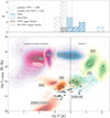 |
Fig. 5. Radio power at 1.4 GHz versus linear size plot (P-D diagram) for different types of RL and RQ AGNs, adapted from Baldi (2023). Points show individual objects and coloured contours represent a smoothed estimator of source density. The different categories of source shown are: CSO (compact symmetric objects), GPS (GHz-peaked spectrum sources), CSS (compact steep spectrum sources), FRI, FRII, RQ quasars, Seyferts and LINERS, and FR0s. The vertical dashed line roughly marks the separation between resolved and unresolved compact sources based on arcsecond angular resolution. The blue dots represent how SUBWAYS AGNs overlap to LINERS & Seyferts, FRIs, FR0s and RQQ. PG1425+267 is a strong outlier, falling on the FRIIs region. Such variety is consistent with the sample being selected based on its X-ray properties. In the upper panel we show the linear size distribution of the sample, with the UFO-subsample (filled histogram) separated from the non-UFO one (barred histogram). The median physical size measured for the UFO subsample is higher (12.35 ± 5 kpc) with respect to the non-UFO one (2.96 ± 1 kpc), potentially supporting multi-phase outflow models (e.g. Crenshaw et al. 2003). Medians are computed taking into account the upper limits through KM survival analysis. Catalogue references: LINERS & Seyferts (Baldi et al. 2018), FR0 (Baldi et al. 2019; Cheng & An 2018); RQQ (Jarvis et al. 2021); GPS (Liu et al. 2007); CSS (Kunert-Bajraszewska et al. 2010); CSO (An & Baan 2012); FRI (Dabhade et al. 2020; Jimenez-Gallardo et al. 2019); FRII (Lao et al. 2024; Fanti et al. 1987). |
By locating the sample in a radio luminosity-linear size (P–D) diagram, as shown in Fig. 5, it is immediately noticeable that SUBWAYS (blue dots) occupies a region wide enough to encompass at least four different classes of objects: classical RQ quasars (RQQ, yellow), low-ionisation nuclear emission-line region galaxies (LINERs; Singh et al. 2013) & Seyferts (brown; Seyfert 1943), low-power Fanaroff-Riley Is (FRI, dark green; Fanaroff & Riley 1974) and Fanaroff-Riley 0 (FR0, orange; Baldi et al. 2016). The only point located in the region occupied by Fanaroff-Riley IIs (FRII; Fanaroff & Riley 1974) is the GRQ PG1425+267, which represents a clear outlier. The sample shows how an X-ray selection picks up a variety of radio-emitting AGNs; therefore, we expect a non-homogeneous classification of the mechanisms responsible for the radio emission. This variety is consistent with the radio intermediate (e.g. Falcke et al. 1996; Yuan et al. 2008) values of RX in SUBWAYS. Interestingly, the points straddle the line between resolved and unresolved compact sources (vertical dashed black line) for telescopes with arcsecond resolving powers (e.g. Baldi 2023). Sub-arcsecond resolution observations may reveal compact jet structures or unresolved winds (Baldi et al. 2015; Baldi 2023; Chen et al. 2024).
5.2. Radio spectral characteristics
Using the present observations, spanning the 145 MHz – 6 GHz interval, we compare the SED slopes in the 145 MHz–1.5 GHz and 1.5–6 GHz ranges (see Table 4) plotting them in Fig. 6 (left, also called colour-colour plot). To further quantify these spectral behaviours, we also compute the spectral curvature (SPC), defined here as the difference between the 1.5–6 GHz and 145 MHz–1.5 GHz spectral indices ( ; Col. 5 of Table 4). In the left panel of Fig. 6, horizontal and vertical lines at 0 and 0.5 define the region where flat spectra are, while we classify as steep slopes above 0.5 and as inverted those below 0 (e.g. Panessa et al. 2022). If the value of SPC is null, the spectrum can be fitted by a single power law across the entire available frequency range, and the points are located along the bisector. Those located below exhibit instead a high frequency curvature and a positive SPC, consistent with spectral ageing of optically thin plasma. The SEDs of the objects above the bisector flatten towards higher frequencies (negative SPC), suggesting a combination of steep and flat components.
 |
Fig. 6. Left: radio colour-colour plots with the 1.5–6 GHz versus 145 MHz – 1.5 GHz spectral slopes. The yellow dots are the resolved objects while the blue ones are the unresolved ones. Dots are substituted with stars for UFO hosts. Upper limits are plotted with an arrow. Right: Histogram showing the distribution of the spectral curvature, defined as |

If the upper limits and uncertainties are properly considered, all but one of the unresolved targets (PG1402+261) fall in the region where the spectral slope is flat in both regimes, indicative of single or multiple self-absorbed components consistent with either a corona or self-absorbed jet. In contrast, the resolved ones are all either steep or curved. This trend, coupled with the considerations on the sizes of Sect. 5.1, and the UFO detection in six of the resolved targets, suggests that compact and unresolved ones tend to exhibit a flat spectrum, typical of nuclear dense regions, whilst, coherently with the elongation of extended targets, star-formation activity or an outflow must be responsible for a steep or curved spectrum. This can be further quantified with a KM survival analysis, which shows that the UFO subsample has a median SPC around 0.11, while it is -0.07 for the other targets. However, also in this case if a log-rank test is performed, the p-value p ∼ 0.15 is insufficient to state whether the UFO subsample belongs to a different distribution.
5.3. SFR contribution to radio emission
First of all, we verify whether SF can be considered the main mechanism for the production of radio emission. We derive the SFR from the 1.4 GHz luminosity following Condon (1992), and taking care of extrapolating the 1.5 GHz luminosity to 1.4 GHz using the spectral indices  listed in Table 4. For the sources exhibiting multiple components we exclude the extranuclear ones, whose morphology clearly suggests an origin not attributable to the AGN host galaxy. The results are in Table 5 (Col. 3).
In the same table (Col. 4) we list the SFR values either based on near-infrared spectra and far-infrared photometry (Zhang et al. 2016), or derived from Wide-field Infrared Survey Explorer (WISE; Wright et al. 2010) flux densities (using Eq. 5 of Cluver et al. 2017). The latter are labelled with.
Radio versus infrared (IR) values are plotted in Fig. 7. Five targets exceed the 3σ uncertainty region, implying that different processes beyond SF are required to explain their radio emission (e.g. White et al. 2017). In all other cases, the targets sit within 3σ of the relation. Despite this, either the radio emission extension, larger than the host galaxy as observed in optical images (see Appendix B), or the flat SED led us to exclude SF as main responsible for the radio emission. Only PG1402+261 and 2MASXJ1402+26 are unresolved (see Appendix B) and exhibit values of  consistent with being dominated by an optically thin component (α ∼ 0.6) at GHz frequencies, making SF a viable source for the production of most radio emission. The overall observed trend suggests that some contribution from nuclear SF cannot be ruled out, though not dominating the emission, and consequently, the SED shape. This confirms the challenges in identifying the origin of radio emission in RQQ and emphasises the importance of employing complementary indicators.
 |
Fig. 7. logSFR derived from the radio luminosity following Condon (1992) against literature values of logSFR derived from IR diagnostics (Zhang et al. 2016). The blue shaded region represents the 1σ, 2σ, 3σ uncertainty on the relation. Some targets, labelled with (*) in Table 5, are not studied in Zhang et al. (2016), thus their SFR has been computed from WISE flux densities according to the computations of Cluver et al. (2017). Numbers refer to single targets as in Table 5. Apart from five targets exceeding the 3σ uncertainty region, SUBWAYS AGNs follow the relation quite well. However, only PG1402+261 (15) and 2MASXJ1402+26 (13) exhibit SEDs consistent with being dominated by SF. |
5.4. X-ray – radio luminosity correlation
In works by Panessa et al. (2007), Laor & Behar (2008), and Panessa & Giroletti (2013), it has been observed that the 5 GHz radio luminosity and the 2–10 KeV X-ray one in RQ AGNs follow the empirical relation LR/LX ∼ 10−5.5 (Laor & Behar 2008), which is remarkably similar to the Güdel–Benz relation observed for coronally active stars (Guedel & Benz 1993). The latter is considered suggestive of a magnetically heated corona: magnetic reconnection releases energy, with a nearly constant fraction converted into heat (seen as X-ray emission) and particle acceleration (seen as synchrotron radio emission).
To test this scenario, we extrapolate the 6 GHz radio luminosities to 5 GHz, using as  those reported in Table 4. In Fig. 8, we plot the 5 GHz radio luminosity against the X-ray one derived in Paper I, and the empirical relation LR/LX ∼ 10−5.5 (dashed black line, with associated 1,2,3σ uncertainties). For the three objects that exhibit extranuclear components, we consider only the luminosity of the nuclear one (A in Fig. 2).
 |
Fig. 8. Correlation between X-ray and radio luminosity. The dashed black line is the relationship found by Laor & Behar (2008) and the grey regions represent the 1σ, 2σ, 3σ uncertainty. The AGNs where the bulk of radio emission is due to SF are highlighted with orange squares while those where the emission is connected to the corona are surrounded by a red diamond. The dashed red line is the RX=–4.5 traditional threshold between RL and RQ AGNs (Terashima & Wilson 2003). Six RL objects exceed the 3σ uncertainty region, but all other SUBWAYS targets follow the LR/LX ∼ 10−5.5 relation. PG0947+396 (6) and PG1352+183 (4) (red diamonds in the left panel), are unresolved and satisfy the expectations for a corona-dominated spectrum at GHz frequencies. The overall trend confirms that RQQ follow the Güdel–Benz relation almost independently on their radio spectral shape (e.g. Laor & Behar 2008; Panessa & Giroletti 2013). |
First, it is possible to appreciate that the six objects exceeding the 3σ uncertainty region are coherently catalogued as RL according to Terashima & Wilson (2003). Specifically, the fraction of UFO hosts deviating from the relation is 3/7, much larger than that of non-UFO hosts (3/15). This supports the interpretation that in AGNs with nuclear winds shocks from winds or small jets dominate radio emission at 5 GHz, and can significantly increase LR relative to LX (e.g. Zakamska et al. 2016; Mancuso et al. 2017; Richards et al. 2021; Baldi et al. 2022).
All the remaining objects closely follow the relation. However, as already mentioned in Sect. 5.1, current models indicate that corona-dominated emission, which is confined to sub-pc scales, should appear unresolved at arcsecond resolution and exhibit a self-absorbed radio spectrum at GHz frequencies, with spectral indices αR ≤ 0.2 (Raginski & Laor 2016; del Palacio et al. 2025). Only PG0947+396 and PG1352+183 (surrounded by red diamonds in Fig. 8) match these predictions and are therefore good candidates for hosting corona-dominated radio emission.
In conclusion, similarly to the discussion related to SF in Sect. 5.3, although the Güdel–Benz relation seems to hold for RQQ almost independently on their spectral shape, a more detailed analysis using complementary diagnostics reveals that the origin of the radio emission cannot be uniquely attributed to coronal processes, highlighting the importance of a careful and multi-approach analysis.
In general, indeed, coronal emission can be more efficiently traced at millimeter wavelengths (100 s GHz), where the millimeter excess eventually dominates and an unbiased and direct view of the corona is possible (Behar et al. 2015; Panessa et al. 2019; Kawamuro et al. 2022; Ricci et al. 2023; del Palacio et al. 2025). Therefore, our current results would be strengthened by a future analysis of the millimeter emission, which could provide proper evidence for a significant coronal contribution to the overall emission.
5.5. Expected radio emission from winds
Based on the results presented so far, while for two sources the radio emission could be explained with SF and for other two with the corona, for all the other objects all the diagnostics suggest the culprit should be an outflow, either in the form of wind or low-power jet. The observational signatures for the two mechanisms are very similar (i.e. steep GHz spectrum and extended emission), making it particularly complicated to disentangle (Wang et al. 2023) unless higher resolution observations are available.
Focusing on the UFO subsample, in this section we explore the interesting possibility that the observed radio emission originates from large-scale winds, which are the galactic-scale continuation of the X-ray nuclear outflows (King & Pounds 2015; Zubovas & Nardini 2020; Longinotti et al. 2023; Zanchettin et al. 2023). We attempt a connection between the kinetic luminosity of the nuclear winds to the properties of the radio emission, assuming that we observe radio synchrotron rising where the nuclear wind shocks the ISM.
As noted in Sect. 5.1, all UFO hosts except PG0947+396 are extended over tens of kpc and show steep SEDs, consistent with large-scale outflows and possibly supporting multi-phase wind models. In order to place more quantitative constraints, we follow Nims et al. (2015). Starting from the energy conserving wind model of Faucher-Giguère & Quataert (2012), the authors propose an estimate for the expected radio luminosity at a frequency ν ≥ νcool (defined as the frequency after which νLν becomes flat)
 (6)
(6)
where ξ−2 is the energy conversion efficiency in units of 10−2, LAGN the AGN bolometric luminosity, and Lk, o the kinetic luminosity of the radio wind. Under energy-conserving assumptions, we obtain LR, exp substituting Lk, o with the value of the X-ray wind (Lk, i) derived for the SUBWAYS UFO subsample (Paper III). In Col. 9 of Table 5 we report for each UFO host the 5% efficiency estimates, with symmetric uncertainty computed as the distance from the 1% and 10% efficiency values, which is a reasonable efficiency range reported in the literature (e.g. Zubovas & King 2012; King & Pounds 2015; Zubovas & Nardini 2020). In Fig. 9 the blue stars represent the comparison between such values and the observed 6 GHz radio luminosity for the UFO subsample (computed on the whole extension of the targets). However, it is unlikely for the winds to maintain the same kinetic luminosity from UFO scales to kpc ones, where some energy dissipation should occur. For this reason, the blue stars should be interpreted as upper limits.
 |
Fig. 9. Expected radio luminosity versus observed one at 6 GHz for the SUBWAYS UFO subsample (M23, blue and red stars) and the comparison samples from Tombesi et al. (2010, T10, grey diamonds) and Zakamska & Greene (2014, Z14, orange empty triangle). For the latter only the median values are plotted. LR, exp is computed as from Eq. 6 with Lk from Paper III in both the energy-conserving (blue stars and light grey diamonds) and momentum-conserving (red stars and dark grey diamonds) scenario. The observed radio luminosity of our sample is included between upper and lower limits and is coherent with recent observations of multi-phase outflows (e.g. Zanchettin et al. 2023; Longinotti et al. 2023). The hypothesis of outflow-driven radio emission is further supported by the extended radio morphology and the steep radio spectral indices of UFO hosts. |
In order to find lower limits as well, we also consider the momentum-conserving scenario (following, e.g. Faucher-Giguère & Quataert 2012 and Zubovas & King 2012). In this case, the kinetic luminosity of the radio outflow Lk, o differs from Lk, i and can be estimated by comparing the momentum rate of the inner and outer wind: Ṗi = Ṗo. We get Lk, o = Lk, i ⋅ (vo/vi). The ratio between the typical velocity of a large-scale wind (ionised, HI or cold molecular) of ∼500 − 2000 km/s (Zakamska & Greene 2014;Morganti et al. 2016; Fiore et al. 2017; Bischetti et al. 2019) and that of a UFO (0.1 − 0.25c Chartas et al. 2002; Tombesi et al. 2012; Paper I) is around 0.01. Therefore, the radio wind roughly preserves only 1% of the nuclear wind power. The results are reported in Col. 9 of Table 5 and are plotted as red stars in Fig. 9.
The observed radio luminosity of our sample is included between the upper and lower limits, coherently with recent observations of multi-phase outflows on single sources (e.g. Tozzi et al. 2021; Bonanomi et al. 2023; Zanchettin et al. 2023; Longinotti et al. 2023, Baldini et al. 2024) that suggest reality actually lies in between the two limiting cases. Therefore, our result is consistent with radio emission being dominated by outflows. In particular, in terms of radio and X-ray properties, our UFO hosts share interesting similarities with IRAS17020+4544 (Longinotti et al. 2023) and NGC 2992 (Zanchettin et al. 2023), both hosting a multi-phase outflow. Moreover, the work by Villar-Martín et al. (2017) on 2MASXJ1653+23, strongly supports an outflow-related scenario.
Following the same procedure described above, we use the Lk values derived in Paper III for the local RQ AGNs belonging to Tombesi et al. (2010) sample to compute the expected radio luminosity. The observed radio luminosity of this set of AGNs is the result of extrapolations based on NASA/IPAC Extragalactic Database (NED) archival data9. In Fig. 9 we plot the upper limits as light grey diamonds and the lower limits as dark grey ones. Once again, with the exception of two cases, the one-to-one line is encompassed by the two threshold values, thus, a reasoning similar to that used for our sample applies here. With an orange triangle, we represent the median values for the sample of 568 luminous obscured QSO studied by Zakamska & Greene (2014, Z14). The authors derive Lk through a detailed analysis of gas kinematics and not from the UFO parameters, thus substituting its value in Eq. (6) we get a direct estimate of how much kinetic energy is converted into radiation.
In general, further modelling is needed to fully explain the complex interplay between the outflow and the ISM. We note that large-scale (∼kpc) radio outflows develop on ∼Myr timescales, much longer than the typical lifetimes of nuclear UFOs (Zubovas & King 2012; King & Pounds 2015; Zubovas & Nardini 2020). This mismatch implies that, if the radio outflow represents the large-scale extension of a nuclear wind, it is more likely associated with a past episode of nuclear activity of comparable intensity, rather than with the currently observed UFO. Alternatively, the observed coexistence of the two outflows may simply reflect physical conditions that favour the production of both phenomena.
To conclude, the above exercise shows that the bulk of radio emission in UFO hosts is consistent with being driven by an evolution of the nuclear wind. In addition we note that within our UFO subsample we detect steep-spectrum features extending beyond the stellar body of the galaxy, matching with outflow expectations. Although all previous observations fit well within a wind scenario, we stress that we cannot rule out the jet scenario based on this analysis. Higher resolution imaging and an estimate of the polarisation fraction may help to distinguish between the two (Wang et al. 2023; Chen et al. 2023; Meenakshi et al. 2024; Chen et al. 2024).
6. Summary and conclusions
We have analysed radio data of the AGNs in the SUBWAYS sample (z = 0.1–0.5, Lbol = 1044.9 − 46.3 erg/s) and investigated the origin of their radio emission, with a focus on radio-UFO connection, exploiting the availability of a unique combination of multi-band observations, as for RQQ the most likely origins considered are star-formation activity, AGN corona, wind, or jets. The radio proprietary data, simultaneously collected with JVLA at 1.5 and 6 GHz, have been complemented with archival images from LoTSS at 145 MHz, and from additional radio surveys (GMRT, RACS, FIRST, and VLASS) to cover a larger frequency range.
Below we summarise our most important results:
– The detection rate in the proprietary data is 100%. This decreases to 94% in LoTSS and even lower values in the other archival data, due to sensitivity limitations.
– The derived radio luminosities (with median values 23.28, 22.70, 22.43 W/Hz at 145 MHz, 1.5 GHz, and 6 GHz respectively; see Fig. 4), together with the radio loudness parameter computed by exploiting the available X-ray data, suggest that the sources can be classified as RQ or intermediate.
– The morphological classifications based on JVLA 6-GHz and LoTSS images are consistent, revealing twelve unresolved sources and ten resolved ones. For the unresolved sources, the upper limits of the emission extension range from ∼1 kpc to < 10 kpc, therefore winds or low-power jets at sub-kpc and/or kpc scales, if present, could not be resolved. The resolved sources have linear sizes from ∼10 kpc to 1000s kpc. One source, PG1425+267, is a Giant Radio QSO, extending for more than 1000 kpc (Fig. 2). This previously unidentified object is a serendipitous discovery of this work, which may be worth a detailed investigation in the future (see also Fig. 5).
– The radio SEDs, the radio colour-colour plots, and the spectral curvature (Fig. 4, left and middle) highlight a variety of spectral shapes, from simple power-laws, suggestive of an optically thin emitting plasma, to inverted and broken spectra, indicating the presence of an optically thick component dominating either at lower or higher frequencies (see Fig. 6). This is a hint of different mechanisms at the origin of the radio emission.
– Interestingly, six out of the seven UFO hosts show extended radio emission with steep spectra, consistent with outflowing optically thin plasma. While more robust conclusions require larger statistics and in-depth analysis, this may hint at a connection between the two phases, or simply reflect a more suitable environment for producing both phenomena.
– For all sources, we tested whether the observed radio emission is consistent with SF through the radio-IR correlation (Fig. 7). Similarly, we placed our targets in the LR − LX plane to verify their location with respect to the Güdel–Benz relation (LR/LX ∼ 10−5.5; Fig. 8).
Overall, by combining the information from the correlations with the spectral and morphological properties, we find that only in two sources the radio emission may be dominated by SF and in the other two by the corona. With the currently available data, a dominant radio emission mechanism can be identified in just four sources (18%), highlighting the difficulty of analysing radio emission in RQQs, and underscoring the importance of employing complementary diagnostics.
– For all the rest it is likely that an outflow, either in the form of wind or jet, is mainly responsible for the radio emission. In particular, for the seven QSO showing UFOs we computed both upper (energy-conserving) and lower (momentum-conserving) limits for the expected wind radio emission. The observed radio luminosities of our sample lie between the upper and lower predicted limits, suggesting that winds might be a viable mechanism for explaining radio emission (Fig. 9). However, because of the huge degeneracy between the observables, we do not exclude the compact jet scenario.
6.1. Future perspectives
To further explore and confirm the results presented in this work, it would be interesting to verify the presence and properties of outflows in other gas phases and test their relation to the observed radio outflows and UFO. As an example, a uniform analysis of the already available optical SDSS spectra would allow us to test whether or not outflows as traced by [OIII] are detected (e.g. Zakamska & Greene 2014).
Also higher resolution observations of unresolved objects could give stronger constraints on their linear sizes, while for the resolved ones with flux densities of the order of mJy (e.g. with JVLA A configuration, e-MERLIN, and VLBI), those may reveal collimated sub-kpc-scale structures, helping to distinguish jets from winds, as noted in Panessa & Giroletti (2013) and Patil et al. (2020). Furthermore, the nuclear radio emission, measured from sub-arcsecond resolution observations, is expected to better correlate with the X-ray one, further supporting the corona scenario in some cases (Chen et al. 2024 ). We stress that future observations at 100–300 GHz with ALMA will be of great importance for more robust estimates of the corona contribution, not only to investigate spectral shapes (because of the lower frequencies sampled by our data a flat spectrum may be hidden) but also correlated mm-X-ray variability.
Finally, both the Next Generation VLA (ngVLA) and Square Kilometer Array (SKA), offering sub-arcsecond resolution (down to mas with ngVLA) and unprecedented sensitivities, will open new avenues for studying compact objects, even at higher redshift, providing the ideal opportunity to extend this kind of radio analysis to larger samples of sources hosting UFOs.
Data availability
Data associated with this article, including supplementary figures (e.g. the full SEDs and radio images), are available in the Zenodo repository, under the Creative Commons License, https://doi.org/10.5281/zenodo.19921061
Acknowledgments
We acknowledge support from PRINMIUR2017PH3WAT (‘Black hole winds and the baryon life cycle of galaxies’). All the italian co-authors from the SUBWAYS collaboration acknowledge support and fundings from Accordo Attuativo ASI-INAF n. 2017-14-H.0. MBrienza and EAmenta acknowledge financial support from INAF under the Mini Grant 2023 funding scheme (project ‘Low radio frequencies as a probe of AGN jetfeedback at low and high redshift’). MBrienza acknowledges financial support from Next Generation EU funds within the National Recovery and Resilience Plan (PNRR), Mission 4 – Education and Research, Component 2 – From Research to Business (M4C2), Investment Line 3.1 – Strengthening and creation of Research Infrastructures, Project IR0000034 – “STILES - Strengthening the Italian Leadership in ELT and SKA”. LOFAR is the Low Frequency Array designed and constructed by ASTRON. It has observing, data processing, and data storage facilities in several countries, which are owned by various parties (each with their own funding sources), and which are collectively operated by the LOFAR ERIC under a joint scientific policy. The LOFAR resources have benefited from the following recent major funding sources: CNRS-INSU, Observatoire de Paris and Université d’Orléans, France; BMFTR, MKW-NRW, MPG, Germany; Science Foundation Ireland (SFI), Department of Business, Enterprise and Innovation (DBEI), Ireland; NWO, The Netherlands; The Science and Technology Facilities Council, UK; Ministry of Science and Higher Education, Poland; The Istituto Nazionale di Astrofisica (INAF), Italy. This research made use of the Dutch national e-infrastructure with support of the SURF Cooperative (e-infra 180169) and the LOFAR e-infra group. The Jülich LOFAR Long Term Archive and the German LOFAR network are both coordinated and operated by the Jülich Supercomputing Centre (JSC), and computing resources on the supercomputer JUWELS at JSC were provided by the Gauss Centre for Supercomputing e.V. (grant CHTB00) through the John von Neumann Institute for Computing (NIC). This research made use of the University of Hertfordshire high-performance computing facility and the LOFAR-UK computing facility located at the University of Hertfordshire and supported by STFC [ST/P000096/1], and of the Italian LOFAR-IT computing infrastructure supported and operated by INAF, including the resources within the PLEIADI special “LOFAR” project by USC-C of INAF, and by the Physics Department of Turin university (under an agreement with Consorzio Interuniversitario per la Fisica Spaziale) at the C3S Supercomputing Centre, Italy. This research is part of the project LOFAR Data Valorization (LDV) [project numbers 2020.031, 2022.033, and 2024.047] of the research programme Computing Time on National Computer Facilities using SPIDER that is (co-)funded by the Dutch Research Council (NWO), hosted by SURF through the call for proposals of Computing Time on National Computer Facilities. VEG acknowledges funding under NASA contract 80NSSC24K1403. This research used data from HST program number 15890, sponsored by the Space Telescope Science Institute, which is operated by the Association of Universities for Research in Astronomy, Incorporated, under NASA contract NAS5-26555. BDM acknowledges support via the Spanish MINECO grants PID2023-148661NB-I00, PID2022-136828NB-C44, and the AGAUR/Generalitat de Catalunya grant SGR-386/2021. MG acknowledges support from the ERC Consolidator Grant BlackHoleWeather (101086804) MP acknowledges support through the grants PID2021-127718NB-I00, PID2024-159902NA-I00, and RYC2023-044853-I, funded by the Spain Ministry of Science and Innovation/State Agency of Research MCIN/AEI/10.13039/501100011033 and El Fondo Social Europeo Plus FSE+. ALL acknowledges support from DGAPA-PAPIIT IA103625. YK acknowledges support form UNAM-PAPIIT grant IN 102023. EB was supported by The Israel Science Foundation (grant No. 2617/25). POP acknowledges support from the french spatial agency CNES and from the “Action Thématique Phénomènes Extrêmes et Multimessager” of the Astronomy-Astrophysics National Programme from INSU/CNRS. GP acknowledges support from the European Research Council (ERC) under the European Union’s Horizon 2020 research and innovation program HotMilk (grant agreement No. 865637) and from the Framework per l’Attrazione e il Rafforzamento delle Eccellenze (FARE) per la ricerca in Italia (R20L5S39T9). LZ acknowledges financial support from the Bando Ricerca Fondamentale INAF 2022 Large Grant “Toward an holistic view of the Titans: multi-band observations of z > 6 QSOs powered by greedy supermassive black holes”, Bando Ricerca Fondamentale INAF 2024 Large Grant “The DEepest study of LUminous QSOs in X-ray at z = 2-7 (DELUX)” and from the European Union – Next Generation EU, PRIN/MUR 2022 2022TKPB2P – BIG-z. FP acknowledges financial support from the Bando Ricerca Fondamentale INAF and "Programma di Ricerca Fondamentale INAF 2023 and 2024.
References
- Alexander, D. M., Hickox, R. C., Aird, J., et al. 2025, New Astron. Rev., 101, 101733 [Google Scholar]
- An, T., & Baan, W. A. 2012, ApJ, 760, 77 [Google Scholar]
- Baldi, R. D. 2023, A&ARv, 31, 3 [NASA ADS] [CrossRef] [Google Scholar]
- Baldi, R. D., Capetti, A., & Giovannini, G. 2015, A&A, 576, A38 [NASA ADS] [CrossRef] [EDP Sciences] [Google Scholar]
- Baldi, R. D., Capetti, A., & Giovannini, G. 2016, Astron. Nachr., 337, 114 [NASA ADS] [CrossRef] [Google Scholar]
- Baldi, R. D., Williams, D. R. A., McHardy, I. M., et al. 2018, MNRAS, 476, 3478 [Google Scholar]
- Baldi, R. D., Capetti, A., & Giovannini, G. 2019, MNRAS, 482, 2294 [NASA ADS] [CrossRef] [Google Scholar]
- Baldi, R. D., Laor, A., Behar, E., et al. 2022, MNRAS, 510, 1043 [Google Scholar]
- Baldini, P., Lanzuisi, G., Brusa, M., et al. 2024, A&A, 686, A217 [NASA ADS] [CrossRef] [EDP Sciences] [Google Scholar]
- Becker, R. H., White, R. L., & Helfand, D. J. 1995, ApJ, 450, 559 [Google Scholar]
- Behar, E., Baldi, R. D., Laor, A., et al. 2015, MNRAS, 451, 517 [NASA ADS] [CrossRef] [Google Scholar]
- Bicknell, G. V. 1994, Australian J. Phys., 47, 669 [Google Scholar]
- Bischetti, M., Piconcelli, E., Feruglio, C., et al. 2019, A&A, 628, A118 [NASA ADS] [CrossRef] [EDP Sciences] [Google Scholar]
- Bonanomi, F., Cicone, C., Severgnini, P., et al. 2023, A&A, 673, A46 [NASA ADS] [CrossRef] [EDP Sciences] [Google Scholar]
- Briggs, D. S. 1995, Am. Astron. Soc. Meeting Abstr., 187, 112.02 [NASA ADS] [Google Scholar]
- Brusa, M., Matzeu, G., Bianchi, S., et al. 2022, Mem. Soc. Astron. It., 93, 48 [Google Scholar]
- Cattaneo, A., Haehnelt, M. G., & Rees, M. J. 1999, MNRAS, 308, 77 [Google Scholar]
- Chartas, G., Brandt, W. N., Gallagher, S. C., & Garmire, G. P. 2002, ApJ, 579, 169 [Google Scholar]
- Chen, S., Laor, A., Behar, E., Baldi, R. D., & Gelfand, J. D. 2023, MNRAS, 525, 164 [Google Scholar]
- Chen, S., Laor, A., Behar, E., et al. 2024, ApJ, 975, 35 [Google Scholar]
- Cheng, X.-P., & An, T. 2018, ApJ, 863, 155 [NASA ADS] [CrossRef] [Google Scholar]
- Cicone, C., Brusa, M., Ramos Almeida, C., et al. 2018, Nat. Astron., 2, 176 [Google Scholar]
- Ciotti, L., Ostriker, J. P., & Proga, D. 2010, ApJ, 717, 708 [Google Scholar]
- Cluver, M. E., Jarrett, T. H., Dale, D. A., et al. 2017, ApJ, 850, 68 [Google Scholar]
- Condon, J. J. 1992, ARA&A, 30, 575 [Google Scholar]
- Crenshaw, D. M., Kraemer, S. B., & George, I. M. 2003, ARA&A, 41, 117 [NASA ADS] [CrossRef] [Google Scholar]
- Cresci, G., Tozzi, G., Perna, M., et al. 2023, A&A, 672, A128 [NASA ADS] [CrossRef] [EDP Sciences] [Google Scholar]
- Dabhade, P., Röttgering, H. J. A., Bagchi, J., et al. 2020, A&A, 635, A5 [NASA ADS] [CrossRef] [EDP Sciences] [Google Scholar]
- del Palacio, S., Yang, C., Aalto, S., et al. 2025, A&A, 701, A41 [NASA ADS] [CrossRef] [EDP Sciences] [Google Scholar]
- Ehlert, D., Oikonomou, F., & Peretti, E. 2025, MNRAS, 539, 2435 [Google Scholar]
- Fabian, A. C. 2012, ARA&A, 50, 455 [Google Scholar]
- Falcke, H., Sherwood, W., & Patnaik, A. R. 1996, ApJ, 471, 106 [Google Scholar]
- Falcke, H., Wilson, A. S., & Simpson, C. 1998, ApJ, 502, 199 [CrossRef] [Google Scholar]
- Fanaroff, B. L., & Riley, J. M. 1974, MNRAS, 167, 31P [Google Scholar]
- Fanti, C., Fanti, R., de Ruiter, H. R., & Parma, P. 1987, A&AS, 69, 57 [NASA ADS] [Google Scholar]
- Faucher-Giguère, C. A., & Quataert, E. 2012, MNRAS, 425, 605 [NASA ADS] [CrossRef] [Google Scholar]
- Fiore, F., Feruglio, C., Shankar, F., et al. 2017, A&A, 601, A143 [NASA ADS] [CrossRef] [EDP Sciences] [Google Scholar]
- Gaspari, M., Tombesi, F., & Cappi, M. 2020, Nat. Astron., 4, 10 [Google Scholar]
- Gianolli, V. E., Bianchi, S., Petrucci, P. O., et al. 2024, A&A, 687, A235 [NASA ADS] [CrossRef] [EDP Sciences] [Google Scholar]
- Giroletti, M., Panessa, F., Longinotti, A. L., et al. 2017, A&A, 600, A87 [NASA ADS] [CrossRef] [EDP Sciences] [Google Scholar]
- Gordon, Y. A., Boyce, M. M., O’Dea, C. P., et al. 2021, ApJS, 255, 30 [NASA ADS] [CrossRef] [Google Scholar]
- Guedel, M., & Benz, A. O. 1993, ApJ, 405, L63 [NASA ADS] [CrossRef] [Google Scholar]
- Hale, C. L., McConnell, D., Thomson, A. J. M., et al. 2021, PASA, 38, e058 [NASA ADS] [CrossRef] [Google Scholar]
- Intema, H. T., Jagannathan, P., Mooley, K. P., & Frail, D. A. 2017, A&A, 598, A78 [NASA ADS] [CrossRef] [EDP Sciences] [Google Scholar]
- Jarvis, M. E., Harrison, C. M., Thomson, A. P., et al. 2019, MNRAS, 485, 2710 [Google Scholar]
- Jarvis, M. E., Harrison, C. M., Mainieri, V., et al. 2021, MNRAS, 503, 1780 [NASA ADS] [CrossRef] [Google Scholar]
- Jimenez-Gallardo, A., Massaro, F., Capetti, A., et al. 2019, A&A, 627, A108 [NASA ADS] [CrossRef] [EDP Sciences] [Google Scholar]
- Karwin, C., Ajello, M., Diesing, R., Caprioli, D., & Chartas, G. 2023, BAAS, 55, 300.03 [Google Scholar]
- Kauffmann, G., & Haehnelt, M. 2000, MNRAS, 311, 576 [Google Scholar]
- Kawamuro, T., Ricci, C., Imanishi, M., et al. 2022, ApJ, 938, 87 [NASA ADS] [CrossRef] [Google Scholar]
- King, A. R., & Pounds, K. 2015, ARA&A, 53, 115 [NASA ADS] [CrossRef] [Google Scholar]
- King, A. R., Lubow, S. H., Ogilvie, G. I., & Pringle, J. E. 2005, MNRAS, 363, 49 [NASA ADS] [CrossRef] [Google Scholar]
- Kormendy, J., & Ho, L. C. 2013, ARA&A, 51, 511 [Google Scholar]
- Kunert-Bajraszewska, M., Gawroński, M. P., Labiano, A., & Siemiginowska, A. 2010, MNRAS, 408, 2261 [NASA ADS] [CrossRef] [Google Scholar]
- Kuźmicz, A., & Jamrozy, M. 2021, ApJS, 253, 25 [CrossRef] [Google Scholar]
- La Franca, F., Melini, G., & Fiore, F. 2010, ApJ, 718, 368 [NASA ADS] [CrossRef] [Google Scholar]
- Lacy, M., Baum, S. A., Chandler, C. J., et al. 2016, BAAS, 227, 324.09 [Google Scholar]
- Lacy, M., Baum, S. A., Chandler, C. J., et al. 2020, PASP, 132, 035001 [Google Scholar]
- Lao, B.-Q., Yang, X.-L., Jaiswal, S., et al. 2024, RAA, 24, 035021 [Google Scholar]
- Laor, A., & Behar, E. 2008, MNRAS, 390, 847 [NASA ADS] [CrossRef] [Google Scholar]
- Liu, X., Cui, L., Luo, W.-F., Shi, W.-Z., & Song, H.-G. 2007, A&A, 470, 97 [NASA ADS] [CrossRef] [EDP Sciences] [Google Scholar]
- Longinotti, A. L., Salomé, Q., Feruglio, C., et al. 2023, MNRAS, 521, 2134 [CrossRef] [Google Scholar]
- Maksym, W. P., Elvis, M., Fabbiano, G., et al. 2023, ApJ, 951, 146 [NASA ADS] [CrossRef] [Google Scholar]
- Mancuso, C., Lapi, A., Massardi, M., & Danese, L. 2017, Workshop sull’Astronomia Millimetrica in Italia, 2 [Google Scholar]
- Matzeu, G. A., Brusa, M., Lanzuisi, G., et al. 2023, A&A, 670, A182 [Google Scholar]
- Mauch, T., & Sadler, E. M. 2007, MNRAS, 375, 931 [Google Scholar]
- McConnell, D., Hale, C. L., Lenc, E., et al. 2020, PASA, 37, e048 [Google Scholar]
- Meenakshi, M., Mukherjee, D., Bodo, G., Rossi, P., & Harrison, C. M. 2024, MNRAS, 533, 2213 [Google Scholar]
- Mehdipour, M., Kriss, G. A., Brusa, M., et al. 2023, A&A, 670, A183 [NASA ADS] [CrossRef] [EDP Sciences] [Google Scholar]
- Mestici, S., Tombesi, F., Gaspari, M., Piconcelli, E., & Panessa, F. 2024, MNRAS, 532, 3036 [NASA ADS] [CrossRef] [Google Scholar]
- Morganti, R. 2017, Front. Astron. Space Sci., 4, 42 [CrossRef] [Google Scholar]
- Morganti, R., Veilleux, S., Oosterloo, T., Teng, S. H., & Rupke, D. 2016, A&A, 593, A30 [NASA ADS] [CrossRef] [EDP Sciences] [Google Scholar]
- Mukherjee, D. 2025, Galaxies, 13, 102 [Google Scholar]
- Murthy, S., Morganti, R., Wagner, A., et al. 2022, Eur. Astron. Soc. Annual Meet., 874 [Google Scholar]
- Nims, J., Quataert, E., & Faucher-Giguère, C. A. 2015, MNRAS, 447, 3612 [NASA ADS] [CrossRef] [Google Scholar]
- Offringa, A. R. 2010, Astrophysics Source Code Library [record ascl:1010.017] [Google Scholar]
- Offringa, A. R., McKinley, B., Hurley-Walker, N., et al. 2014, MNRAS, 444, 606 [Google Scholar]
- Padovani, P. 2017, Nature, 1, 0194 [Google Scholar]
- Panessa, F., & Giroletti, M. 2013, MNRAS, 432, 1138 [NASA ADS] [CrossRef] [Google Scholar]
- Panessa, F., Barcons, X., Bassani, L., et al. 2007, A&A, 467, 519 [NASA ADS] [CrossRef] [EDP Sciences] [Google Scholar]
- Panessa, F., Baldi, R. D., Laor, A., et al. 2019, Nat. Astron., 3, 387 [Google Scholar]
- Panessa, F., Chiaraluce, E., Bruni, G., et al. 2022, MNRAS, 515, 473 [Google Scholar]
- Patil, P., Nyland, K., Whittle, M., et al. 2020, ApJ, 896, 18 [NASA ADS] [CrossRef] [Google Scholar]
- Perley, R. A., & Butler, B. J. 2013, ApJS, 204, 19 [Google Scholar]
- Pounds, K. 2014, Space Sci. Rev., 183, 339 [Google Scholar]
- Raginski, I., & Laor, A. 2016, MNRAS, 459, 2082 [CrossRef] [Google Scholar]
- Ricci, C., Chang, C.-S., Kawamuro, T., et al. 2023, ApJ, 952, L28 [NASA ADS] [CrossRef] [Google Scholar]
- Richards, G. T., McCaffrey, T. V., Kimball, A., et al. 2021, AJ, 162, 270 [NASA ADS] [CrossRef] [Google Scholar]
- Sabater, J., Best, P. N., Hardcastle, M. J., et al. 2019, A&A, 622, A17 [NASA ADS] [CrossRef] [EDP Sciences] [Google Scholar]
- Seyfert, C. K. 1943, ApJ, 97, 28 [NASA ADS] [CrossRef] [Google Scholar]
- Shimwell, T. W., Röttgering, H. J. A., Best, P. N., et al. 2017, A&A, 598, A104 [NASA ADS] [CrossRef] [EDP Sciences] [Google Scholar]
- Shimwell, T. W., Hardcastle, M., Tasse, C., et al. 2022, A&A, 659, A1 [NASA ADS] [CrossRef] [EDP Sciences] [Google Scholar]
- Shimwell, T. W., Hardcastle, M. J., Tasse, C., et al. 2026, A&A, 707, A198 [NASA ADS] [CrossRef] [EDP Sciences] [Google Scholar]
- Singh, R., van de Ven, G., Jahnke, K., et al. 2013, A&A, 558, A43 [NASA ADS] [CrossRef] [EDP Sciences] [Google Scholar]
- Speranza, G., Ramos Almeida, C., Acosta-Pulido, J. A., et al. 2022, A&A, 665, A55 [NASA ADS] [CrossRef] [EDP Sciences] [Google Scholar]
- Terashima, Y., & Wilson, A. S. 2003, ApJ, 583, 145 [Google Scholar]
- The CASA Team, Bean, B., Bhatnagar, S., et al. 2022, PASP, 134, 114501 [NASA ADS] [CrossRef] [Google Scholar]
- Tombesi, F., Cappi, M., Reeves, J. N., et al. 2010, A&A, 521, A57 [NASA ADS] [CrossRef] [EDP Sciences] [Google Scholar]
- Tombesi, F., Cappi, M., Reeves, J. N., & Braito, V. 2012, MNRAS, 422, L1 [Google Scholar]
- Tombesi, F., Tazaki, F., Mushotzky, R. F., et al. 2014, MNRAS, 443, 2154 [NASA ADS] [CrossRef] [Google Scholar]
- Tombesi, F., Meléndez, M., Veilleux, S., et al. 2015, Nature, 519, 436 [NASA ADS] [CrossRef] [Google Scholar]
- Tozzi, G., Cresci, G., Marasco, A., et al. 2021, A&A, 648, A99 [NASA ADS] [CrossRef] [EDP Sciences] [Google Scholar]
- Ulivi, L., Venturi, G., Cresci, G., et al. 2024, A&A, 685, A122 [NASA ADS] [CrossRef] [EDP Sciences] [Google Scholar]
- Venturi, G., Marconi, A., Mingozzi, M., et al. 2021, IAU Symp., 359, 464 [Google Scholar]
- Villar-Martín, M., Emonts, B., Cabrera Lavers, A., et al. 2017, MNRAS, 472, 4659 [Google Scholar]
- Wang, A., An, T., Jaiswal, S., et al. 2021, MNRAS, 504, 3823 [NASA ADS] [CrossRef] [Google Scholar]
- Wang, A., An, T., Zhang, Y., et al. 2023, MNRAS, 525, 6064 [NASA ADS] [CrossRef] [Google Scholar]
- White, S. V., Jarvis, M. J., Kalfountzou, E., et al. 2017, MNRAS, 468, 217 [Google Scholar]
- Wright, E. L., Eisenhardt, P. R. M., Mainzer, A. K., et al. 2010, AJ, 140, 1868 [Google Scholar]
- Yamada, S., Kawamuro, T., Mizumoto, M., et al. 2024a, ApJS, 274, 8 [NASA ADS] [CrossRef] [Google Scholar]
- Yamada, T., Sakai, N., Inoue, Y., & Michiyama, T. 2024b, ApJ, 968, 116 [Google Scholar]
- Yuan, W., Zhou, H. Y., Komossa, S., et al. 2008, ApJ, 685, 801 [NASA ADS] [CrossRef] [Google Scholar]
- Zakamska, N. L., & Greene, J. E. 2014, MNRAS, 442, 784 [Google Scholar]
- Zakamska, N. L., Lampayan, K., Petric, A., et al. 2016, MNRAS, 455, 4191 [Google Scholar]
- Zanchettin, M. V., Feruglio, C., Massardi, M., et al. 2023, A&A, 679, A88 [NASA ADS] [CrossRef] [EDP Sciences] [Google Scholar]
- Zhang, Z., Shi, Y., Rieke, G. H., et al. 2016, ApJ, 819, L27 [NASA ADS] [CrossRef] [Google Scholar]
- Zubovas, K., & King, A. 2012, ApJ, 745, L34 [Google Scholar]
- Zubovas, K., & Nardini, E. 2020, MNRAS, 498, 3633 [Google Scholar]
Throughout the paper, when we do not distinguish between winds and jets we refer to them more generally as outflows.
VLA CASA Calibration Pipeline 5.6.2.
The Kaplan-Meier estimator is a non-parametric method adapted to estimate the cumulative distribution function (CDF) for data containing non-detects (left-censored data). The median survival time is estimated as the point where the CDF drops to 0.5.
A two-sided Fisher exact test on the 2×2 contingency table ([6, 1],[4, 11]) yields p ≈ 0.020 (the association is marginally significant at the ∼2% level).
Appendix A: Tables
Imaging parameters.
All Tables
All Figures
|
Fig. 1. Bolometric luminosity as a function of redshift. The grey contours highlight the AGNs of Yamada et al. (2024a, Y24), the red ones are the data from Laor & Behar (2008, LB08), and those in purple the data from Panessa & Giroletti (2013, PG13). We choose LB08 and PG13 as a comparison for the study of the X-ray-radio luminosity correlation. Then we plot the objects in the SUBWAYS sample (blue empty dots) and a comparison sample from Tombesi et al. (2010, T10, black empty diamonds). UFO hosts are marked by stars and triangles in SUBWAYS and T10 respectively. |
| In the text | |
|
Fig. 2. Images of the ‘multi-component’ sources. Colours at 6 GHz with σrms ⋅ [ − 3, 3, 6, 12, 24, 48, 96] contours at 1.5 GHz (white) and 145 MHz (green). The beams are shown in the bottom-left corner of each panel. Labels A, B, and C mark distinct radio components: A denotes the nuclear (core) component spatially coincident with the optical AGN position, while B and C denote spatially-separated extranuclear components (i.e. features that are not coincident with the optical/IR nucleus and that extend beyond the host’s optical light profile) likely related to AGN outflows. |
| In the text | |
|
Fig. 3. Image of PG1427+480, showing the extended emission detected in the north-east direction of the target, which is located in the lower-right region of the image. Colours at 6 GHz with σrms ⋅ [ − 3, 3, 6, 12, 24, 48, 96] contours at 1.5 GHz (white) and 145 MHz (6″in green, 20″in cyan). The beams are shown in the bottom-left corner of the panel. The black cross marks the optical position of the AGN. |
| In the text | |
|
Fig. 4. Left: Spectral index distribution of the sample. The filled histogram represents the values computed between 1.5 and 6 GHz, while the barred one those computed between 145 MHz and 1.5 GHz. Middle: Histogram comparing the total radio luminosities of the sample. Blue: 145 MHz. Violet: 1.5 GHz. Green: 6 GHz. The upper limits at 145 MHz have been excluded. Right: Radio loudness parameter distribution of the sample. The convention followed is RX = log (LR(6 cm)/LX(2 − 10 KeV)) (Terashima & Wilson 2003). The filled histogram represents the values of RX computed for the UFO hosts, and the barred histogram those derived for the non-UFO hosts. The vertical red line marks the –4.5 limit set by Terashima & Wilson (2003). RQ AGNs tend to dominate the sample, while RL AGNs represent only a small fraction, specifically 6/21 with the original limit RX = –4.5. |
| In the text | |
|
Fig. 5. Radio power at 1.4 GHz versus linear size plot (P-D diagram) for different types of RL and RQ AGNs, adapted from Baldi (2023). Points show individual objects and coloured contours represent a smoothed estimator of source density. The different categories of source shown are: CSO (compact symmetric objects), GPS (GHz-peaked spectrum sources), CSS (compact steep spectrum sources), FRI, FRII, RQ quasars, Seyferts and LINERS, and FR0s. The vertical dashed line roughly marks the separation between resolved and unresolved compact sources based on arcsecond angular resolution. The blue dots represent how SUBWAYS AGNs overlap to LINERS & Seyferts, FRIs, FR0s and RQQ. PG1425+267 is a strong outlier, falling on the FRIIs region. Such variety is consistent with the sample being selected based on its X-ray properties. In the upper panel we show the linear size distribution of the sample, with the UFO-subsample (filled histogram) separated from the non-UFO one (barred histogram). The median physical size measured for the UFO subsample is higher (12.35 ± 5 kpc) with respect to the non-UFO one (2.96 ± 1 kpc), potentially supporting multi-phase outflow models (e.g. Crenshaw et al. 2003). Medians are computed taking into account the upper limits through KM survival analysis. Catalogue references: LINERS & Seyferts (Baldi et al. 2018), FR0 (Baldi et al. 2019; Cheng & An 2018); RQQ (Jarvis et al. 2021); GPS (Liu et al. 2007); CSS (Kunert-Bajraszewska et al. 2010); CSO (An & Baan 2012); FRI (Dabhade et al. 2020; Jimenez-Gallardo et al. 2019); FRII (Lao et al. 2024; Fanti et al. 1987). |
| In the text | |
|
Fig. 6. Left: radio colour-colour plots with the 1.5–6 GHz versus 145 MHz – 1.5 GHz spectral slopes. The yellow dots are the resolved objects while the blue ones are the unresolved ones. Dots are substituted with stars for UFO hosts. Upper limits are plotted with an arrow. Right: Histogram showing the distribution of the spectral curvature, defined as |
| In the text | |
|
Fig. 7. logSFR derived from the radio luminosity following Condon (1992) against literature values of logSFR derived from IR diagnostics (Zhang et al. 2016). The blue shaded region represents the 1σ, 2σ, 3σ uncertainty on the relation. Some targets, labelled with (*) in Table 5, are not studied in Zhang et al. (2016), thus their SFR has been computed from WISE flux densities according to the computations of Cluver et al. (2017). Numbers refer to single targets as in Table 5. Apart from five targets exceeding the 3σ uncertainty region, SUBWAYS AGNs follow the relation quite well. However, only PG1402+261 (15) and 2MASXJ1402+26 (13) exhibit SEDs consistent with being dominated by SF. |
| In the text | |
|
Fig. 8. Correlation between X-ray and radio luminosity. The dashed black line is the relationship found by Laor & Behar (2008) and the grey regions represent the 1σ, 2σ, 3σ uncertainty. The AGNs where the bulk of radio emission is due to SF are highlighted with orange squares while those where the emission is connected to the corona are surrounded by a red diamond. The dashed red line is the RX=–4.5 traditional threshold between RL and RQ AGNs (Terashima & Wilson 2003). Six RL objects exceed the 3σ uncertainty region, but all other SUBWAYS targets follow the LR/LX ∼ 10−5.5 relation. PG0947+396 (6) and PG1352+183 (4) (red diamonds in the left panel), are unresolved and satisfy the expectations for a corona-dominated spectrum at GHz frequencies. The overall trend confirms that RQQ follow the Güdel–Benz relation almost independently on their radio spectral shape (e.g. Laor & Behar 2008; Panessa & Giroletti 2013). |
| In the text | |
|
Fig. 9. Expected radio luminosity versus observed one at 6 GHz for the SUBWAYS UFO subsample (M23, blue and red stars) and the comparison samples from Tombesi et al. (2010, T10, grey diamonds) and Zakamska & Greene (2014, Z14, orange empty triangle). For the latter only the median values are plotted. LR, exp is computed as from Eq. 6 with Lk from Paper III in both the energy-conserving (blue stars and light grey diamonds) and momentum-conserving (red stars and dark grey diamonds) scenario. The observed radio luminosity of our sample is included between upper and lower limits and is coherent with recent observations of multi-phase outflows (e.g. Zanchettin et al. 2023; Longinotti et al. 2023). The hypothesis of outflow-driven radio emission is further supported by the extended radio morphology and the steep radio spectral indices of UFO hosts. |
| In the text | |
Current usage metrics show cumulative count of Article Views (full-text article views including HTML views, PDF and ePub downloads, according to the available data) and Abstracts Views on Vision4Press platform.
Data correspond to usage on the plateform after 2015. The current usage metrics is available 48-96 hours after online publication and is updated daily on week days.
Initial download of the metrics may take a while.