| Issue |
A&A
Volume 709, May 2026
|
|
|---|---|---|
| Article Number | A46 | |
| Number of page(s) | 15 | |
| Section | Extragalactic astronomy | |
| DOI | https://doi.org/10.1051/0004-6361/202558652 | |
| Published online | 01 May 2026 | |
The AGN nature of strong C III] emitters in the early Universe with JWST
1
INAF – Osservatorio Astronomico di Roma, via Frascati 33, 00078 Monteporzio Catone, Italy
2
Dipartimento di Fisica, Università di Roma Sapienza, Città Universitaria di Roma – Sapienza, Piazzale Aldo Moro, 2, 00185 Roma, Italy
3
Physics Department, Tor Vergata University of Rome, Via della Ricerca Scientifica 1, 00133 Rome, Italy
4
Institute of Physics, Laboratory for Galaxy Evolution and Spectral Modelling, EPFL, Observatoire de Sauverny, Chemin Pegasi 51, 1290 Versoix, Switzerland
5
University of the Pacific, Stockton, CA 90340, USA
6
Instituto de Astrofísica de Andalucía (IAA-CSIC), Glorieta de la Astronomía s/n, 18008 Granada, Spain
7
Department of Physics and Astronomy, University of Kansas, Lawrence, KS 66045, USA
8
Department of Astronomy and Astrophysics, The Pennsylvania State University, University Park, PA 16802, USA
9
Institute for Computational and Data Sciences, The Pennsylvania State University, University Park, PA 16802, USA
10
Institute for Gravitation and the Cosmos, The Pennsylvania State University, University Park, PA 16802, USA
11
NSF’s NOIRLab, Tucson, AZ 85719, USA
12
Institute for Astronomy, University of Edinburgh, Royal Observatory, Edinburgh EH9 3HJ, UK
13
Department of Astronomy, The University of Texas at Austin, Austin, TX, USA
14
Cosmic Frontier Center, The University of Texas at Austin, Austin, TX, USA
15
University of Massachusetts Amherst, 710 North Pleasant Street, Amherst, MA 01003-9305, USA
16
Laboratory for Multiwavelength Astrophysics, School of Physics and Astronomy, Rochester Institute of Technology, 84 Lomb Memorial Drive, Rochester, NY 14623, USA
17
Space Telescope Science Institute, 3700 San Martin Drive, Baltimore, MD 21218, USA
18
INFN – Rome Tor Vergata, Via della Ricerca Scientifica 1, 00133 Rome, Italy
19
Department of Physics, 196A Auditorium Road, Unit 3046, University of Connecticut, Storrs, CT 06269, USA
20
School of Astronomy and Space Science, University of Chinese Academy of Sciences (UCAS), Beijing 100049, China
21
National Astronomical Observatories, Chinese Academy of Sciences, Beijing 100101, China
22
Institute for Frontiers in Astronomy and Astrophysics, Beijing Normal University, Beijing 102206, China
★ Corresponding author: This email address is being protected from spambots. You need JavaScript enabled to view it.
Received:
18
December
2025
Accepted:
9
March
2026
Abstract
The semi-forbidden C III] λλ1907,1909 doublet is a key tracer of high-ionisation emission in the early Universe. We present a study of C III] emission in galaxies at z = 5 − 7, using publicly available JWST/NIRSpec prism data from programmes including CEERS, JADES, and RUBIES, along with data from the ongoing CAPERS survey. We built a sample of 61 C III]-emitting galaxies, and we classified them as star-forming galaxies (SFGs) or active galactic nucleus (AGN) host galaxies using (1) rest-frame UV and optical emission-line diagnostic diagrams, and (2) the presence or absence of broad Balmer emission lines. The UV diagnostics are based on the combination of the rest-frame equivalent width (EW) of C III] versus the ratio C III]/He IIλ1640, and the EW of C IV versus the ratio C IV/He IIλ1640. For optical diagnostics, we used the OHNO diagram, which combines four optical emission lines that span a range in ionization potential: [O III] λ5008, Hβ, [Ne III] λ3869, and [O II] λλ3726,3729. We find that it separates AGNs from SFGs with low efficiency. Half of the sources in our sample (29 out of 61 galaxies) exhibit at least one secure indication of AGN activity, while 13 are potential AGNs based on the C III] diagnostic. We derived physical properties, including stellar mass and star formation rate, through spectral energy distribution modelling with BAGPIPES. Our analysis shows that JWST is uncovering a population of strong C III] emitters at high redshift (5 < z < 7) with a median EW of 22.8 Å (16th–84th percentile: 12.5–51.5 Å). This EW exceeds than that of a control sample of C III] emitters at intermediate redshift (3 < z < 4), which have a median EW of 4.7 Å. For the same range of MUV, the C III] EW increases by ∼0.67 dex from 3 < z < 4 to 5 < z < 7, indicating strong redshift evolution in the line strength. We also find that C III] emitters span the full range of the star-forming main sequence, where the majority of galaxies below the sequence have a high C III] EW. Finally, we identify five sources in our sample as little red dots (LRDs) according to the selection criteria in the literature; four of these have already been identified as LRDs, while one is presented here for the first time.
Key words: techniques: photometric / techniques: spectroscopic / galaxies: active / galaxies: evolution / galaxies: high-redshift
© The Authors 2026
 Open Access article, published by EDP Sciences, under the terms of the Creative Commons Attribution License (https://creativecommons.org/licenses/by/4.0), which permits unrestricted use, distribution, and reproduction in any medium, provided the original work is properly cited.
This article is published in open access under the Subscribe to Open model. This email address is being protected from spambots. You need JavaScript enabled to view it. to support open access publication.
1. Introduction
The epoch of reionization (EoR) represents a pivotal phase in cosmic history, following the initial ‘cosmic dawn’. During this era, ionising radiation from the first stars and galaxies, and potentially from the earliest active galactic nuclei, ended the cosmic dark ages and drove the transition of the intergalactic medium (IGM) from neutral to ionised at z ≳ 5.3 (e.g. Bosman et al. 2022; Spina et al. 2024; Becker et al. 2015). Studying the sources responsible for this process – whether primordial starbursts or active galactic nuclei (AGNs) – is crucial to understanding the drivers of reionization (e.g. Hegde et al. 2024). However, observing these distant sources presents significant challenges. Emission lines provide a powerful window into the physical conditions of galaxies, encoding information about their ionisation state, gas density, metallicity, and radiation field. During the EoR, observational access is largely limited to rest-frame UV diagnostics, which makes the choice of emission lines particularly important. Although Lyα is often the brightest UV line, its resonant nature causes it to be heavily attenuated and scattered by neutral hydrogen in the IGM, complicating its interpretation as a probe of intrinsic galaxy properties. We therefore focus on alternative UV lines such as C III] λλ1907,1909, which arise from nebular gas and provide more direct constraints on the physical conditions within high-redshift galaxies (e.g. Le Fèvre et al. 2019).
The semi-forbidden doublet of doubly-ionised carbon, C III] λλ1907,1909 (hereafter C III]), offers a powerful opportunity to reveal AGN hosts and star-forming galaxies (SFGs) at high-z. It is typically the second-brightest UV emission line after Lyα, which makes it readily observable. Additionally, C III] traces the gas with high-energy radiation, since it requires photons with energies between ∼24.4 eV and 47.9 eV (the range needed to create and excite C2+). Such energies arise from intense radiation fields typically associated with either AGNs or young, metal-poor starburst galaxies.
Extensive pre-James Webb Space Telescope (JWST; Gardner et al. 2023) observations of galaxies at z ∼ 2 − 4, using both ground-based spectroscopy and Hubble Space Telescope observations at low redshift, have established the diagnostic power of rest-frame UV emission lines for identifying ionisation sources and constraining galaxy physical conditions. Studies have shown that C III] is sensitive to metallicity, ionisation parameter, and the hardness of the ionising radiation field in SFGs, with particularly strong emission observed in young, metal-poor systems (e.g. Stark et al. 2014; Nakajima et al. 2018). Recently Cunningham et al. (2024) analysed a sample of 62 sources showing C III] emission (as well as Lyα) at 3 < z < 4 from the VIMOS survey of the CANDELS fields (VANDELS). These sources have rest-frame (C III]) equivalent widths (EWs) between ≃1–15 Å, with a median value of 4.7 Å. Only a small fraction of the sources (10 out of 62, i.e. around 14) were identified as AGNs, with the remainder dominated by star formation (see also Le Fèvre et al. 2019).
These pre-JWST results demonstrate that UV emission-line diagnostics provide a robust framework for distinguishing star formation from AGN ionisation, motivating their application to JWST observations of galaxies in the reionization era.
The JWST has fundamentally transformed our ability to study these C III] emitters at high-z. For the first time, we have access to a powerful, sensitive infrared instrument capable of efficiently observing the rest-frame UV and optical spectra of high-redshift galaxies simultaneously. Because the C III] feature is redshifted into the near-infrared for objects during the EoR, JWST instruments are ideally suited for its detection and characterisation. The JWST not only detects faint C III] emission but also measures it alongside other key UV lines. These include C IVλλ1548,1551, He IIλ1640, O III] λλ1661, 1666, and [Ne V] λ3426 (hereafter C IV, He II, O III], and [Ne V], respectively). These lines are key for robust diagnostic analyses (e.g. Hirschmann et al. 2019, 2023; Feltre et al. 2016; Gutkin et al. 2016; Nakajima & Maiolino 2022). A central challenge, even with JWST capabilities, is distinguishing the nature of the ionising sources in C III] emitters. At high redshifts, classical optical diagnostic diagrams such as the BPT (Baldwin, Phillips & Terlevich 1981) and VO87 (Veilleux & Osterbrock 1987) (Baldwin et al. 1981; Veilleux & Osterbrock 1987) diagrams become less efficient due to a combination of factors, including different physical conditions such as low metallicity (e.g. Übler et al. 2023) and the shifting of key optical lines out of the observable spectral range of the telescope. Furthermore, applying these diagnostics often requires high spectral resolution that is not always available for deep, large-scale spectroscopic surveys. We therefore investigated the utility and limitations of the OHNO diagram for our sample (see Section 4.3), noting that recent studies show that the chosen line ratios are largely degenerate with respect to the ionisation parameter (Cleri et al. 2025).
In this work, we use JWST data to advance the study of galaxies during the EoR by focusing on the properties of C III]-emitting galaxies. Given the challenges of distinguishing AGNs and star-formation origins at high redshift, a primary goal of our work is to apply optical and UV diagnostics to identify and distinguish these sources. We perform spectral energy distribution (SED) fitting to estimate physical properties such as stellar mass. Finally, we examine the connection between C III] emitters and a newly discovered population known as little red dots (LRDs).
The structure of this paper is as follows. Section 2 describes the observational data and sample selection and outlines the spectroscopic and photometric analysis methodology, including the use of LIME for emission-line fitting and BAGPIPES for SED modelling. We present our main results, as well as the stacking procedure, in Section 3, with the application of AGN diagnostics detailed in Section 4. Section 5 explores the relationship between C III] emitters and LRDs, and Section 6 discusses the nature of the C III] emitters. We summarise our findings and discuss potential extensions in Section 7.
Throughout this work, we assume a ΛCDM (Lambda-Cold Dark Matter) cosmological model with the parameters H0 = 70 km s−1 Mpc−1, Ωm = 0.3, and ΩΛ = 0.7. Magnitudes are expressed in the AB system (Oke & Gunn 1983), and EWs are reported in the rest frame.
2. Sample selection and data analysis
2.1. Spectroscopic data
For our analysis, we used JWST-NIRSpec prism data. The prism, unlike the gratings, provides continuous, wide wavelength coverage (0.6–5.3 μm) in a single exposure, which is essential for capturing the full suite of diagnostic lines across our redshift range. The trade-off for this extensive coverage is the low and strongly wavelength-dependent spectral resolution: the resolving power increases nearly linearly from R ∼ 30 at 0.6 μm to R ∼ 300 at 5.3 μm. Across our redshift range (5 < z < 7), this corresponds to a velocity width of ∼5000–6000 km s−1 at rest-frame UV wavelengths and ∼1000–1400 km s−1 at rest-frame optical wavelengths. Although this resolution limits detailed kinematic measurements and measurements of closely spaced lines, it is suited for detecting and measuring integrated emission line fluxes for AGN diagnostics and population studies, as performed here.
The tail end of the EoR, concluding around z ≳ 5.3 (e.g. Bosman et al. 2022), provides a crucial window to study the galaxies responsible for the cosmic transition. The redshift range 5 < z < 7 targeted in this work was strategically chosen because it probes this final phase of reionization and offers a key observational advantage: it allows the simultaneous observation of both rest-frame UV emission lines (such as C III] and He II) and optical lines (such as Hβ and [O III] λ5008, hereafter [O III]) required for our AGN diagnostic diagrams, as well as Hα for investigating broad-line AGN components. We used publicly available JWST-NIRSpec-prism data from the CANDELS-Area Prism Epoch of Reionization Survey (CAPERS; GO-6368; PI: Mark Dickinson), an ongoing Cycle 3 JWST programme that observes up to 10000 high-redshift galaxies split across the Cosmic Evolution Survey (COSMOS), the Ultra-deep Survey (UDS), and the Extended Groth Strip (EGS) fields in the PRISM/CLEAR configuration. In this work, we focus on sources with 5 < z < 7 from all three fields and identify a total of 549 galaxies.
To complement the CAPERS data1, we collected all publicly available JWST spectroscopic observations in the UDS, EGS, COSMOS, Goods North, Goods South, and A2744 fields from v3 of the DAWN JWST archive (DJA, Heintz et al. 2024; de Graaff et al. 2025a) up to 24 February 2025. We limited our selection to robust (grade = 3) spectroscopically identified galaxies at 5 < z < 7, to match the CAPERS redshift range. We identified a total of 1307 galaxies (corrected for duplicates).
Combining the DJA and CAPERS samples, we find a total of 1856 unique galaxies.
2.2. Emission line measurements with LIME
To identify C III] emitters in the CAPERS and DJA parent samples, we used the A LIne MEasuring library (LIME; Fernández et al. 2024), following a multi-step process. As a first step, we processed all galaxies using the spectroscopic redshifts provided by the DJA and CAPERS catalogues. The LIME library defines rest-frame spectral windows for each emission feature, including the line region and adjacent continuum bands. The software models emission lines using Gaussian profiles, each described by three free parameters: amplitude, central wavelength, and velocity dispersion (σ). For closely spaced emission lines, such as the [O III] λλ4960,5008 doublet, LIME can account for blending by performing a multi-component Gaussian fit when specified. This initial analysis yields key measurements, including fluxes, equivalent widths, velocity dispersions, and line-based redshifts for various rest-UV and optical emission lines, such as C III] and [O III].
We then refined the DJA and CAPERS redshifts using the values from LIME, ensuring that the new redshifts did not deviate excessively from the original values by requiring a difference of less than 0.016 (corresponding to a maximum velocity offset of 600–800 km/s for C III]). We also verified that the lines used to define the redshift were consistent with the instrumental resolution by comparing the measured full width at half maximum (FWHM) of the line with the instrumental resolution2 (FWHMinst).
We required S/N > 23 on the flux of C III] and identified a sample of 61 C III] emitters (which will be presented in more detail in Section 3). We then corrected the absolute flux calibration of the C III] emitter spectra for potential slit losses by comparing them with the broad-band photometry from Merlin et al. (2024). We generated synthetic photometry by integrating each spectrum over standard NIRCam filter bandpasses of F090W, F115W, F150W, F200W, F277W, F356W, and F444W. We computed a single, wavelength-independent correction factor – the weighted average of all available filters – by comparing synthetic and observed fluxes. We then applied this correction factor to the entire spectrum and its uncertainties. This process corrects the absolute flux scale without affecting spectral features such as EWs or the UV β slope. We provide additional details in Appendix A.
2.3. Measurement of broad Hα
We used a Markov chain Monte Carlo (MCMC) approach to compare models with and without a broad Hα Gaussian component and to establish which model best reproduces the observed data. We did not include the Hβ line in this modelling because it is fainter and observed at lower spectral resolution, so we expected any broad component to be undetectable there if it was absent in Hα. The first model fits the total observed Hα emission line with a single Gaussian, described by three free parameters (peak flux, central wavelength, and FWHM) and a power-law continuum, described by its slope and a normalisation coefficient; this results in a total of five free parameters. We set uniform priors for the peak flux, FWHM, and continuum parameters and adopted a Gaussian prior for the central wavelength, centred on the source redshift with dispersion equal to the redshift uncertainty. The second model adds a second Gaussian component to model the broad emission, characterised by its own amplitude and velocity dispersion and sharing the central wavelength as the narrow line. This results in seven free parameters: the amplitudes and velocity dispersions of the narrow and broad components, the common central wavelength, and the two continuum parameters (slope and normalisation coefficient). We set analogous priors as fin the first model, except for the FWHM prior of the narrow component,  . This prior spans a continuous interval of one to two spectral resolution elements. We computed the size of a spectral resolution element at the line’s central wavelength by accounting for the wavelength-dependent variation of the prism resolution, i.e. converting R to FWHM at a given wavelength using the R–λ relation from Jakobsen et al. (2022). At the Hα wavelength, the prism spectral resolution corresponds to a velocity width of ∼1000–1400 km s−1 across our redshift range (5 < z < 7). We derived the best-fitting values and associated errors from the 50th, 16th, and 84th percentiles of the posterior distributions, respectively.
We calculated the Bayesian information criterion (BIC), calculated from the χ2 values of each fit and used it as our primary diagnostic. A ΔBIC = BICnarrow − BICbroad > 6 indicates strong evidence for a broad component, while ΔBIC > 2 suggests tentative evidence (e.g. Juodžbalis et al. 2026). As a secondary check, we compared the reduced χ2 values, favouring the model with the lower value. We also visually inspected the residuals and line profiles to ensure consistency.
2.4. Physical properties with BAGPIPES
We estimated galaxy physical properties using the Bayesian Analysis of Galaxies for Physical Inference and Parameter EStimation (BAGPIPES; Carnall et al. 2018) code to fit photometric data. Our analysis uses the photometric catalogue presented by Merlin et al. (2024), comprising 16 bands from the HST and JWST, drawn from large public surveys including CANDELS (Grogin et al. 2011; Koekemoer et al. 2011) and CEERS (Bagley et al. 2023; Finkelstein et al. 2025), which provide continuous wavelength coverage from 0.44 to 4.44 μm. The filter set includes HST/ACS optical bands (F435W, F606W, F775W, F814W), HST/WFC3 near-infrared bands (F105W, F125W, F140W, F160W), and JWST/NIRCam bands (F090W, F115W, F150W, F200W, F277W, F356W, F410M, F444W). These data cover the same fields as our spectroscopic sample and enables robust SED fitting across the rest-frame UV to optical for 55 of the 61 galaxies in our z = 5 − 7 sample. The catalogue provides total flux measurements and associated uncertainties in microJanskys (μJy).
We performed SED fitting with BAGPIPES, assuming a delayed-τ star formation history, characterised by galaxy age (0.001 Gyr up to the Universe’s age at the observed redshift) and the τ parameter (0.1–10 Gyr), which controls the star formation timescale. We allowed the total stellar mass formed to vary between 101 and 1015 M⊙, and we explored the metallicity within 0–0.5 times the solar value. We modelled dust attenuation using a Calzetti law (e.g. Calzetti et al. 2000), with AV ranging from 0 to 2 magnitudes (e.g. Markov et al. 2025). We also included nebular emission, with the ionisation parameter log U varying from –4 to 0. Fitting this model to the observed data, BAGPIPES infers the best-fitting set of physical parameters that describe the galaxy’s evolution and current state.
To account for potential AGN activity, we expanded the base model by adding the AGN model described in Carnall et al. (2023), which includes a continuum component modelled as a broken power law with a break at 5100 Å and broad Hα and Hβ emission. Free parameters included the Hα flux and line width, the continuum flux at 5100 Å, and the power-law slopes. We derived the broad Hβ flux from Hα assuming case B recombination and the same line width. In this expanded model, the parameter space for the stellar and nebular components remained the same as in the base model, and we applied dust attenuation exclusively to these components.
We estimated the UV absolute magnitude for each galaxy from the best-fitting SED template using a top-hat filter centred on λrest = 1500 Å with a width of 100 Å. We then converted this to an absolute magnitude using
 (1)
(1)
where m1500 is the apparent magnitude at λrest = 1500 Å and DL is the luminosity distance in parsecs. We estimated the uncertainty on MUV by simple error propagation on the flux following the approach of Llerena et al. (2025), Pahl et al. (2025).
We derived Hα-based star-formation rates (SFRs) by estimating the Hα emission line flux, applying dust corrections using the AV values estimated by BAGPIPES SED fitting, converting to Hα luminosity LHα, and then to SFR using the calibration from Reddy et al. (2022):
 (2)
(2)
Finally, we used BAGPIPES best-fitting models to derive the stellar mass of our sources. For each galaxy, we compared reduced χ2 (χ2red) values derived for fits performed with and without an AGN component, and adopted the stellar mass from the fit with the lowest χ2red (see Sect. 4.4 for details).
Since no photometry is available for CEERS-1324, we performed a spectroscopic fit with BAGPIPES. We included a second order polynomial with Gaussian priors on its coefficients to correct for potential flux calibration mismatches between the model and the observed spectrum, and a white-noise scaling model to represent wavelength-independent uncertainties. We also included the instrumental resolution curve extracted from the JWST/NIRSpec prism dispersion file to convolve the spectral model to the appropriate resolving power across the fitted wavelength range. To promote fast convergence, we fixed log U to a value of −2, which is close to the average ionisation parameter derived from the photometric SED fitting of the other sources in our sample.
3. C III] emitter sample
We identified 61 C III] emitters out of 1896 galaxies analysed with LIME. Fig. 1 shows two examples of our spectra.
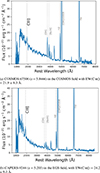 |
Fig. 1. Rest-frame spectra of C III]-emitters from different surveys. Both panels show the rest-frame wavelength in Ångströms on the x axis and flux density in units of 10−21 erg s−1 cm−2 Å−1 on the y axis. |
Our sample comprises galaxies spanning z = 5 − 7, with the distribution peaking around z = 5.25 (Figure 2). The sample includes 24 galaxies with z > 6 and 37 galaxies with z ≤ 6, yielding a median redshift of 5.87.
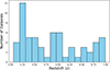 |
Fig. 2. Redshift distribution of the galaxy sample. The histogram shows the number of galaxies as a function of redshift between z = 5 and z = 7, with a pronounced peak at z = 5.25. |
The EW(C III]) values in our sample span nearly two orders of magnitude, from 2.5 Å to 284.2 Å. The distribution has a median EW of 22.8 Å (16th–84th percentile: 12.5–51.5 Å) and a mean of 39.2 Å. We compared the rest-frame EW(C III]) values of our 5 < z < 7 galaxies against lower-redshift (3 < z < 4) emitters from the VANDELS survey (Cunningham et al. 2024). At fixed MUV, our sample exhibits systematically stronger EW(C III]) than the lower-redshift analogues (see Figure 3). The median EW for the combined 3 < z < 4 sample is 4.7 Å compared to 22.8 Å for our sample, corresponding to an increase of ∼0.67 dex in the C III] EW from z = 3 − 4 to z = 5 − 7, indicating strong redshift evolution in the line strength.
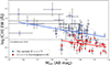 |
Fig. 3. Rest-frame C III] EW (in Å) versus absolute UV magnitude (MUV; AB mag). Blue points show the sample of C III] emitters at z = 5 − 7. Red points show the VANDELS sample compiled by Cunningham et al. (2024) at z = 3 − 4. Contour plots and linear regression fits are also shown. |
This enhancement could be due to several factors. Observational biases may contribute, because JWST/NIRSpec prism spectroscopy lacks the sensitivity to detect C III] emission with low EWs (EW ≤ 5–10 Å) at these redshifts, potentially leading to incomplete sampling of the low-EW population. In fact, the EW(C III]) measured from the stacked spectrum of non-detections in our sample (Table C.2) is 5.7 ± 0.3 Å, consistent with the typical values at lower redshifts. This confirms that the low-EW population is likely undersampled due to observational limitations. From the completeness analysis, we estimate a detection limit of 8.1 Å, below which the number counts drop to 50% of the maximum frequency. This selection bias means that we are incompletely sampling the low-EW population at z = 5 − 7.
Nevertheless, the absence of similarly high EW values at lower redshifts may indicate a genuine evolutionary trend. The systematically elevated EWs in our high-redshift sample suggest that galaxies at z = 5 − 7 inherently produce stronger C III] emission.
This evolutionary trend aligns with the results from Roberts-Borsani et al. (2024), and may reflect harder radiation fields, lower metallicities, and/or higher ionisation parameters in the early Universe (e.g. Llerena et al. 2022; Nakajima et al. 2018, 2023; Trump et al. 2023; Sanders et al. 2023, 2024; Curti et al. 2023; Cameron et al. 2023).
Alternatively, the different distribution of EW(C III]) might arise because the JWST sample is actually dominated by AGNs rather than SFGs. Indeed, JWST has revealed the existence of a much larger population of high-redshift AGNs than previously expected (e.g. Juodžbalis et al. 2026; Scholtz et al. 2025; Treiber et al. 2025). Our analysis of the C III] properties will help discriminate between the two possibilities.
We also find a significant correlation between EW(C III]) and MUV in our sample, with a slope of 0.126 ± 0.039. This indicates that fainter galaxies (higher MUV values) exhibit stronger C III] emission relative to their continuum, consistent with the behaviour observed in lower-redshift samples. The Cunningham et al. (2024) sample shows a similar positive correlation, with a slope of 0.109 ± 0.039.
Figure 4 shows the star formation mass sequence diagram (SFR vs. stellar mass; Speagle et al. 2014), illustrating where our C III] emitters lie relative to the general population. We colour-coded our galaxies by the EW(C III]) value. We excluded the C III] emitters without available photometry as SED fitting cannot be performed, and we also excluded our LRD sample (Section 5). In the background, a reference sample of spectroscopic galaxies from the same surveys with 5 < z < 7 represents the general parent population. We also show the main sequence line from Calabrò et al. (2024) derived with Hα-based SFRs for a similar spectroscopic sample. Our C III] emitters are distributed across the entire main sequence, showing no strong systematic trend. However, galaxies lying below the Calabrò et al. (2024) line are more likely to exhibit strong EWs, although such emitters are not restricted to this region.
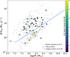 |
Fig. 4. Star formation rate (SFR) versus stellar mass from our sample compared to the star formation of field galaxies at z = 5 − 7. Our sample is colour-coded by the rest-frame C III] EW. The general parent population in the same redshift range appears as grey circles. The blue line represents the relationship found by Calabrò et al. (2024), derived with SFR based on Hα for a similar spectroscopic sample. |
To characterise the global spectral features of the C III] emitters, we performed a stacking analysis, binning the sample by their EW(C III]). This allowed us to increase the S/N of the final spectra. We separated the galaxies into two EW(C III]) bins. Since the median EW in the sample is 23 Å, we performed a stack of weak emitters (EW ≤ 22.8 Å) and strong emitters (EW > 22.8 Å), populated by 31 and 30 galaxies, respectively.
The stacking uses a non-weighted scheme. We first shifted individual spectra into the rest-frame using the systemic redshift based on [OIII] and then resampled them onto a common grid. To define a common wavelength grid for the stacking, we first computed the minimum spectral sampling (Δλ) of each individual spectrum in the observed frame > 1400 (1 + z) Å, which corresponds to 70.54 Å. We then divided by (1 + zmean) to obtain the characteristic rest-frame wavelength spacing, where zmean is the mean redshift of the stacked galaxies in each bin. This sampling provides a representative dispersion for the sample and ensures a consistent grid when resampling spectra obtained with the NIRSpec/prism, whose wavelength dispersion varies with wavelength and redshift. The mean systemic redshift of the sample is zmean ∼ 6.06 for the strong emitters and zmean ∼ 5.71 for the weak emitters. We then normalised the spectra to the median flux between 2700 and 2800 Å, a wavelength range that is free of bright emission lines in the individual spectra. We took the final flux at each wavelength as the median of all the individual flux densities. We estimated the 1-σ error spectrum by a bootstrap re-sampling of the individual flux densities for each wavelength and calculating the standard deviation of the resulting median-stacked spectra. Fig. 5 shows the stacked spectra.
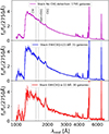 |
Fig. 5. Stacked spectra for non-C III] emitters (top panel), weak (middle panel), and strong (bottom panel) C III] emitters. In all panels, the shaded regions represent the 1σ uncertainty of the stacking. The dashed vertical black line indicates the position of the rest-frame UV emission lines. |
We also stacked the spectra of non-C III] emitters (those galaxies from our parent sample with S/N < 2 on the flux of C III]). This subset includes 1795 galaxies with a mean redshift zmean = 5.8, after excluding overlapping sources from multiple surveys. We followed the same methodology as for C III] emitters; the resulting stacked spectrum is shown in the top panel in Fig. 5.
We applied the same methodology as for individual galaxies, using LIME (Fernández et al. 2024) to measure the fluxes and EWs of the UV and optical emission lines. For the considered emission lines, we assumed a single-Gaussian model.
4. AGN diagnostics
Understanding whether C III] emission in galaxies is powered by star formation or AGNs is crucial to interpreting their physical conditions. AGNs can significantly enhance high-ionisation emission lines, including C III], because of their hard ionising spectra, while SFGs produce these lines through stellar processes such as massive young stars and shocks. Without distinguishing AGNs from SFGs, studies of C III] emitters risk misattributing the ionisation source, leading to incorrect estimates of stellar masses and SFRs. Therefore, robust AGN diagnostics are essential.
4.1. Broad emission lines and black hole mass estimates
Broad Hα emission is a classic signature of an AGN (where the broad-line region is unobscured), originating from high-velocity gas in the vicinity of the central supermassive black hole (e.g. Vanden Berk et al. 2001; Lynden-Bell 1969). A broad component, typically with a FWHM of several thousand km/s, indicates gas motions governed by the black hole (BH) gravitational potential and provides strong evidence for AGN activity distinct from star formation. Detecting such broad lines, even in low-resolution spectra, provides strong evidence for AGN activity and is a key diagnostic in distinguishing AGNs from SFGs.
Detecting broad emission is particularly challenging with the NIRSpec prism because of its lower spectral resolution, which can blur broad and narrow features together. Despite this limitation, our three-tier approach (Section 2.3) allows us to robustly identify broad Hα emission in 15 out of 60 galaxies, including five LRDs (see Section 5).
When assessing the presence of a broad Hα component, we additionally verified that the apparent line broadening was not driven by contamination from the merged [N II] λ6585 (hereafter [N II]) emission. Among the 15 sources exhibiting a broad Hα component, three have FWHM values below 2000 km s−1, while the remaining sources show FWHM > 2000 km s−1, which cannot be reproduced by [N II] emission alone. For the three lower-FWHM sources, we performed an additional fit that included only a narrow Hα component and the [N II] doublet and compared it with a model that included both narrow and broad Hα components following the same procedure as above. We find that only GDS-202208 is better described by the [N II] model, and we therefore exclude it from the broad Hα galaxy sample. We detect no comparable broad component in the [O III] emission line, making an origin from outflows or complex narrow-line region kinematics unlikely.
An example of a galaxy exhibiting a broad Hα component is shown in Figure 6, which presents the source GDS-13704 from the GOODS-South field at a z = 5.93. This source has a ΔBIC = 34.5, indicating strong evidence for the presence of a broad component.
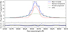 |
Fig. 6. Example of a galaxy with a significant broad Hα component: GDS-13704 at z = 5.93. The black line shows the observed spectrum. The blue line represents the best-fit model using a double Gaussian profile. The red line shows the narrow component, while the green line corresponds to the broad component. The x axis shows the rest-frame wavelength in Angstroms, and the y axis shows the flux density in units of 10−21 erg s−1 cm−2 Å−1. This source has a ΔBIC = 34.5, providing strong evidence for the presence of broad-line emission. |
Based on the detected broad Hα emission, we derive BH masses for our 14 galaxies by adopting the relation from Equation (1) of Reines & Volonteri (2015). From the BH mass measurements, we calculate the Eddington luminosity as LEdd = 1.3 × 1038 (MBH, Hα/M⊙) erg s−1. We also derive the bolometric luminosity (Lbol) of the AGNs using the continuum luminosity at 3000 Å and the bolometric correction from Richards et al. (2009). From the LEdd and Lbol, we infer the corresponding Eddington ratios λEdd = Lbol/LEdd. We report the results in Table 1. The last five galaxies correspond to LRDs (Section 5), and we omit their stellar masses due to the large uncertainties in the estimates.
Properties of the C III] emitters with a broad Hα component.
Figure 7 shows our sample of C III] emitters in the MBH − M* diagram, compared with other known AGNs at 4 < z < 11 (Juodžbalis et al. 2026; Übler et al. 2023; Maiolino et al. 2025; Marshall et al. 2025; Parlanti et al. 2024; Rinaldi et al. 2025; Übler et al. 2025; Fei et al. 2025; Bogdán et al. 2024; Larson et al. 2023; Akins et al. 2025; Harikane et al. 2023; Kocevski et al. 2023; Kokorev et al. 2024; Tripodi et al. 2025; Ding et al. 2023; Harikane et al. 2023; Wang et al. 2024; Übler et al. 2024; Maiolino et al. 2024) and a compilation of quasars (QSOs) at 2 < z < 7 (Tripodi et al. 2024, and references therein). For hosts, we adopted the dynamical mass as an upper limit for the stellar mass, since stellar masses are not yet available for these sources. We excluded the five LRDs from the plot because of the significant uncertainty in deriving their stellar mass (see Section 5). Similarly to the majority high-z AGNs, our C III] emitters lies above the local relations (Kormendy & Ho 2013; Reines & Volonteri 2015; Greene et al. 2020), indicating a more rapid evolution of BHs relative to their hosts in this early phase of their evolution. We also tested for a possible relation between the ratio of log(MBH, Hα/M*) and the EW(C III]) and find no significant correlation.
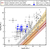 |
Fig. 7. Black hole mass versus stellar mass. Blue stars show our nine C III] emitters with broad Hα emission, compared with 4 < z < 10 AGNs (grey squares; Harikane et al. 2023; Kocevski et al. 2023; Juodžbalis et al. 2026; Wang et al. 2024; Übler et al. 2024; Akins et al. 2025; Kokorev et al. 2023; Larson et al. 2023; Bogdán et al. 2024; Maiolino et al. 2024, full references in the text), a compilation of 2 < z < 7 QSOs (grey cross; treated as upper limits; Tripodi et al. 2024, see references therein), and local scaling relations (dashed grey, solid red and dotted yellow lines, respectively from refs. Kormendy & Ho 2013; Reines & Volonteri 2015; Greene et al. 2020). |
4.2. UV diagnostics
Other reliable AGN diagnostics rely on UV lines. Specifically, diagnostics involving the He II and [Ne V] lines show an effective discriminating power (e.g. Feltre et al. 2016; Gutkin et al. 2016). Unfortunately, these lines are not easily detected individually. For He II, the prism resolution is insufficient to separate it from O III] in most cases, especially at low S/N.
We employed two AGN diagnostics based on the He II emission line: EW(C III]) versus C III]/He II and EW(C IV]) versus C IV/He II (Nakajima et al. 2018). We adopted model grids for SFGs and AGNs that are an extended version of the models from Nakajima & Maiolino (2022). We generated SFG models using CLOUDY with BPASS v2.2.1 stellar populations Eldridge et al. (2017), Stanway & Eldridge (2018) covering a range of metallicities (Z ≈ 0.0007–1 Z⊙), ionisation parameters (log U ≈ –3 to –1), and stellar ages (1–10 Myr). The AGN models employ the CLOUDY AGN continuum, including the big bump and power-law components, with metallicities Z ≈ 0.0007–2 Z⊙ and log U ≈ –2.5 to –0.5. These extended models are described in detail in Arevalo-Gonzalez et al. (2025). To constrain the He II flux, we measured the merged flux of the (He II + O III]) feature and then estimated the He II contribution alone, based on the O III]/He II ratio measured in the stacked spectra (Appendix B). Specifically, we used the derived O III]/He II ratio of 0.87 ± 0.38. This value is similar to the ratios previously found in both star-forming and AGN host galaxies at intermediate redshift (e.g. Amorín et al. 2017; Llerena et al. 2022).
Figure 8 shows EW(C III]) versus C III]/He II. Of our 39 galaxies, four have S/N > 2 for the He II line, while the remainder show upper limits of the He IIλ1640 line. The figure also includes results for the stacks. Using the commonly employed demarcation lines from Nakajima et al. (2018), we find that one galaxy resides in the star-forming region. Twenty-two additional galaxies occupy the AGN region. Even accounting for potential shifts to higher x-axis values due to their upper limits, their high EW(C III]) values would maintain their classification as AGNs. Four of these galaxies fall outside the plotted range of the diagram. They have upper limits for the He II line and are positioned on the left side of the plot. For clarity, we set axis limits to exclude these points from the displayed range. Additionally, we identify 16 galaxies currently located in the AGN region that could potentially shift into the SFG region. For the purposes of this analysis, we classify them as potential AGN. Red markers highlight C III] emitters that exhibit a broad Hα component. We plotted ten out of 14 sources, where seven are AGNs and three are potential AGNs according to the UV diagram. This demonstrates a good agreement between the two diagnostics.
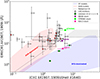 |
Fig. 8. UV-diagnostic diagram showing the EW of C III] versus the ratio C III]/He II. The SFG and AGN models are from Nakajima & Maiolino (2022), while the dashed black line is from Nakajima et al. (2018). Values measured from the stacked spectra are shown as purple (weak stack), light green (strong stack), and pink (no C III] stack) points, with lower-redshift stacks (darker green) from Llerena et al. (2022). The C III] emitters with a broad Hα are plotted as red diamonds. Four galaxies that lie outside the range of the plot and have upper limits on He II emission are GDS-5093, RUBIES-49140, CAPERS-101195, and CAPERS-9244, with C III]/He II values of 0.04, 0.09, 0.02, and 0.01, respectively; the EWs of C III] are listed in Table C.1. |
An examination of the stacked spectra reveals that the strong C III] stack clearly resides in the AGN region, while the weak C III] stack lies within the SFG region, near the demarcation line. The stack of non-C III] emitters lie in the SFG region, very close to the stacked spectra of lower-redshift galaxies presented in Llerena et al. (2022).
Figure 9 presents an alternative UV diagnostic, showing EW(C IV) versus C IV/He II ratio. In the six galaxies showing C IV emission, He II remains undetected, providing lower limits on the C IV/He II ratios. Although these six galaxies lie in the AGN region of the diagram, their lower limits on the x axis mean they could shift into the mixed, SF dominated region, and they also exhibit large uncertainties on the y axis. Overall, we consider this analysis inconclusive for individual sources. We also include the results from the stacks, as in previous analyses. The strong stack again falls well within the AGN region, while the weak stack occupies a mixed region containing both AGN and SFG models. The non-C III] stack is also located in this mixed region, although the C IV line remains undetected.
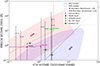 |
Fig. 9. UV-diagnostic diagram showing the EW of C IV versus the ratio C IV/He II. The demarcation lines are given by Hirschmann et al. (2019). Models and stacks are the same as in Figure 8. |
4.3. OHNO diagram
The OHNO diagram (Backhaus et al. 2022) has been proposed as a potential AGN diagnostic, using the ratios [Ne III] λ3869/[O II] λλ3726,3729 and [O III]/Hβ. These ratios rely on four rest-optical emission lines that are relatively accessible at high redshift. A key advantage of the OHNO diagram over the traditional BPT diagram (Baldwin et al. 1981) is that it does not rely on Hα and [N II], which can blend together in low-resolution spectra and fall outside the observable range of JWST at z > 7.
Although useful, the OHNO diagram is more sensitive to the gas-phase metallicity and ionisation parameter than to the fundamental source of the ionising spectrum itself, since the selected line ratios are largely degenerate in their ionisation potential (Cleri et al. 2025). Therefore, although we used it for comparison, we place greater diagnostic weight to UV line ratios in our analysis. To assess systematic uncertainties in this diagnostic, we examined how our results changed under different AGN and SFG models.
For 41 sources in our sample, we can measure or place meaningful limits on both line ratios; we present the results in Figure 10. One galaxy falls outside the plotted range of the diagram; it is an upper limit positioned on the right side of the graph. For clarity, we set axis limits that exclude this point from the displayed range.
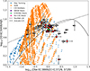 |
Fig. 10. Star-forming galaxy (SFG) models from Gutkin et al. (2016) and AGN models from Plat et al. (in prep.) in the OHNO diagram. The dashed black demarcation line is from Feuillet et al. (2024), while the solid black line is from Arevalo-Gonzalez et al. (2025). Stacked measurements are shown as purple (weak stack), light green (strong stack), and pink (no C III] stack) points. The C III] emitters with a broad Hα are plotted as red diamonds. The values for RUBIES-15072 (outside the plot range) are log10([Ne III] λ3869/[O II] λλ3726,3279) = 2.22 and log10([O III]/Hβ) = 0.83 ± 0.08. |
We first plotted the separation lines from Feuillet et al. (2024), derived empirically from SDSS spectroscopic data, and from Arevalo-Gonzalez et al. (2025), which is based on the previously mentioned photoionisation models of Nakajima & Maiolino (2022). We also plotted SFG models from Gutkin et al. (2016) and, for AGN, a new set of models from Plat et al. (in prep.), which are based on the recent AGN spectra of Kubota & Done (2018) and incorporate dependencies on BH mass and Eddington ratio. For both sets of models, we used an ionisation parameter range of −4 < log U < −2. The metallicity ranges are 0.0001 < Z < 0.03 for the Plat et al. models and 0.0002 < Z < 0.03 for the Gutkin et al. models. We assumed ranges of 3 < log(MBH/M⊙) < 9 for the BH mass and −1.5 < log(λEdd) < 2 for the Eddington ratio. The Gutkin et al. models additionally assume an initial mass function (IMF) with an upper mass cutoff of 300 M⊙, a constant SFR, and stellar population ages of 3 Myr and 10 Myr.
As shown in Figure 10, we identify 20 AGNs (using the Feuillet et al. (2024) line) or 22 AGNs (using the Arevalo-Gonzalez et al. (2025) line): according to these diagnostics, sources above the line are classified as AGNs, while sources below the line could originate from SFGs or AGNs.
When comparing our sources with the Plat and Gutkin models, the situation is less clear: only two sources fall in the AGN-only region, while the remaining sources occupy the mixed region containing both AGN and SFG models. This discrepancy highlights that the OHNO diagram is less efficient at identifying AGNs than UV diagrams because the results depend strongly on the adopted models or demarcation lines.
We also highlight in red the C III] emitters that show a broad Hα component. Of the 12 sources that can be placed on the diagram, four fall in the AGN region, while the remaining eight lie in the mixed region. All 12 lie in the mixed region when compared with the Plat and Gutkin photoionisation models.
Examination of the stacked spectra shows that the three stacks fall below both diagnostic lines, placing them close together in the mixed region. This again demonstrates the lower efficiency of the OHNO diagram compared to the UV diagrams, which separate the stacks into distinct regions.
4.4. AGN component from SED fitting
An additional diagnostics for characterising our sources comes from SED fitting. Specifically, we compared the quality of the best-fit SED photometric models with and without an AGN component, using their reduced χ2 values. Photometric data were unavailable for six sources, leaving 55 sources for this comparison.
For 13 sources, the fit including an AGN component yielded a lower reduced χ2 value, indicating that this component is necessary to reproduce the photometry. Amongst those 13 sources, 11 show additional secure AGN indicators, either from the presence of a broad emission line component, from the UV diagram, or both. This set includes the five identified LRDs (see the next section). The remaining two sources, namely GDS-210003 and CAPERS-41455, are also classified as potential AGNs based on the UV diagram.
For this set, we calculated the fractional contribution of the AGN component to the optical rest-frame continuum for eight of the 13 cases (excluding the LRDs, for which a reliable AGN model has not been established). The AGN fraction is measured from the photometric spectrum at a rest-frame wavelength of 5500 Å, chosen to avoid contamination from emission lines. We find an average AGN fraction of 62.3%, with a standard deviation of 26.3%.
For the other 42 sources, the SED fitting without the AGN component is preferred. Within this group, 25 have previous AGN indications (15 confirmed AGNs and ten potential AGNs). For most of these (14 confirmed AGNs and seven potential AGNs), the difference in the reduced χ2 between the two fits is small, indicating that the SED fitting does not strongly favour either model. In contrast, for the only galaxy classified as a secure SFG in the UV diagram, GDS-202208, shows a very large reduced χ2 difference of 160, strongly favouring the model without an AGN component, consistent with the emission line diagnostics. Finally, the galaxy RUBIES-127820, which could not be placed on previous diagnostic plots, is also best fit by a model without an AGN, although the χ2 difference is small.
We conclude that SED fitting based on photometry alone securely identifies approximately one third of our AGN population. This fraction could be significantly improved by incorporating spectro-photometric SED fitting. Based on our analysis, when a source is classified as an AGN by SED fitting, the identification is reliable, and no SFGs are misclassified as AGNs.
5. LRDs amongst C III] emitters
In under three years of operation, the JWST has delivered numerous surprises. Amongst these is the discovery of a completely new population of red, compact sources that are unexpectedly abundant in the early phase of our Universe, the so-called little red dots (e.g. Matthee et al. 2024; Pérez-González et al. 2024). These galaxies are very compact sources, exhibiting a characteristic V-shaped SED and, in most cases, broad hydrogen emission lines with FWHM ≈ 2–3 103 km s−1, interpreted as evidence of AGN activity (see e.g. Kocevski et al. 2025).
Current analyses (e.g. Kocevski et al. 2025) reveal that over 80% of LRDs exhibit broad-line features when brown dwarf contaminants are excluded. A recent model that reproduces most of the observed spectro-photometric features proposes a BH star (BH*) scenario as the engine of LRDs, in which a BH is embedded in a thick, dense gas envelope that produces the Balmer break and associated absorption features (Inayoshi & Maiolino 2025; Naidu et al. 2025; de Graaff et al. 2025b). Despite these advances, fundamental questions persist regarding the physical nature of their obscuring material and the role of LRDs in cosmic evolution.
Using the classification criteria of Kocevski et al. (2025) and Barro et al. (2026), which rely on photometric data to identify LRD candidates, we examined our sample of C III] emitters for LRDs. Nine sources satisfy this photometric selection. To confirm the LRD nature, we also used available spectroscopic data to estimate both the UV and optical slopes, masking emission lines. We fitted the slopes as power laws using an MCMC approach.
We confirm that five of the nine LRD candidates met the colour requirements spectroscopically, with UV slopes −2.8 < βUV < −0.37 and optical slopes βopt > 0. Four were previously identified as LRDs in the literature, and one is a new identification from the CAPERS survey. Figure 11 shows the spectra of these candidates. Standard SED fitting with Bagpipes using photometric data alone fails to accurately reproduce the observed photometry for these LRDs. Although spectrophotometric fitting improves the fit, purely stellar models remain inadequate. Despite ongoing effort to characterise LRDs (e.g. Inayoshi et al. 2025), current SED fitting tools (e.g. Bagpipes, Prospector, Beagle, and Galfit) lack appropriate AGN models tailored for LRDs, preventing reliable mass estimates. Consequently, we exclude these sources from the Main Sequence diagram, as their derived stellar masses remain uncertain.
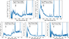 |
Fig. 11. Rest-frame spectra of the five little red dots identified in our sample. From left to right, top to bottom: COSMOS-61234, CAPERS-35805, RUBIES-49140, GDS-13704, and UNCOVER-41225. |
Among the known LRDs at z > 7 in the literature, two show C III] emission (e.g. Jones et al. 2026; Morishita et al. 2026). Additionally, new spectroscopic observations of the Bullet Cluster have identified an LRD at z = 5.3 with C III] emission (e.g. Tripodi et al. 2025). These data became available after we began our analysis.
Overall the fraction of LRDs in our sample of C III] emitters is low (less than 10%). Together with the relatively sparse detection of C III] in LRD spectroscopic samples (around 20% and primarily in redder LRDs; Barro et al. (2026)), confirms that although the C III] emitters and LRDs are both AGN-dominated, they trace distinct populations.
6. The nature of C III] emitters
To assess the presence of AGNs within our sample of C III] emitters, we combined the complementary diagnostics described in the previous sections. We detect broad Hα emission in 14 sources; this represents a lower limit because we used prism spectroscopic observations. These 14 sources are considered secure AGNs. From the UV diagnostics involving C III], we securely classify 22 galaxies as AGNs, out of 39 galaxies that can be meaningfully placed on the diagram, with additional 16 identified as potential AGNs. All sources with broad Hα that could be included in the C III] diagnostic show a consistent AGN classification. The C IV-based diagnostic is limited by the small number of detections; however, all fall within the AGN-dominated region. Importantly, the C IV-based classification is in agreement with the C III]-based diagnostic.
Combining all diagnostics, we find that roughly half of the sources in our sample – 29 out of 61 galaxies – exhibit at least one secure indication of AGN activity, with an additional 13 classified as potential AGNs, based on the C III] diagnostic. These factions are significantly higher than the typical AGN fraction in the general population at similar redshift (Juodžbalis et al. 2026).
Table C.1 summarises the diagnostic results. This group also includes the five sources identified as LRDs, all of which exhibit broad-line components. Although we demonstrate that the OHNO diagram is highly unreliable, most of the sources classified as AGNs by the Arevalo-Gonzalez et al. (2025) demarcation line are also confirmed as AGNs by more robust diagnostics.
Examining the stacked spectra, the OHNO diagram places all three stacks slightly below both demarcation lines, within the mixed region and very close to each other. As expected, the UV diagnostics display more distinct behaviour. Figure 8 shows that the strong C III] stack clearly lies within the AGN region, while the weak C III] stack occupies the star-forming region but remains close to the demarcation line. The stack of non-C III] emitters is located well within the star-forming region, in good agreement with the stacked spectra of lower-redshift galaxies from Llerena et al. (2022). Similarly, in Figure 9, the strong stack is again within the AGN region, the weak stack occupies a mixed zone containing both AGN and SFG models, and the non-C III] emitters remain consistent with SFGs, plotted as upper limits due to the non-detection of the C IV line.
Sect. 4.4 demonstrates that SED fitting using photometry alone robustly identifies roughly one third of the AGN that are identified spectroscopically. This result could likely be improved through spectro-photometric analysis.
Overall, our C III]–emitting sources are predominantly AGNs. This explains the observed EWs compared to those of cosmic noon galaxies with similar MUV in the VANDELS survey (Cunningham et al. 2024; Llerena et al. 2022), where star-forming systems dominate. A VANDELS-like population of galaxies with modest C III] emission likely exists at high redshift; indeed, the stacked spectrum of galaxies without individual line detections shows weak C III] emission (EW(C III]) ≃ 5 Å) and lies consistently within the star-forming regions of all diagnostic diagrams.
Our JWST high-redshift sample also contains a subset of SFGs with high EW(C III]) that are absent in the VANDELS sample. This discrepancy may reflect differences in ISM conditions at very high redshift, such as harder ionising radiation fields, lower metallicities, or higher electron densities (e.g. Llerena et al. 2022; Nakajima et al. 2018).
7. Summary and conclusions
We present a systematic study of C III] emission in 5 < z < 7 galaxies, using JWST/NIRSpec prism spectroscopy. From a parent sample of 1896 galaxies, we identify 61 robust C III] emitters. We measured emission line fluxes and equivalent widths using LIME, and derived physical properties (e.g. stellar masses and star formation rates) through SED fitting with BAGPIPES. Our approach reveals a sample of high-z C III] emitters that show significantly higher rest-frame equivalent widths than C III] emitters at lower redshifts with a similar MUV range (see Figure 3). Although the prism resolution limited our ability to probe low-EW emission lines, none of the intermediate redshift VANDELS sources exhibit EWs above ≃ 10 − 15 Å. This results in a small overlap between the two samples.
The C III] emitters span the full range of the star-forming main sequence, showing no substantial differences in position from the parent population.
To understand the nature of our C III] emitters, particularly relative to the lower redshift sample, we employed multiple AGN diagnostics, including optical and UV emission lines. These diagnostics indicate that AGN activity is common in our C III] emitters. We detect broad emission lines in 14 objects; however, the limited spectral resolution of NIRSpec/prism reduces sensitivity, making this a lower limit on the true number of broad-line sources. The C III] diagnostics classify 22 sources as secure AGNs and 13 additional sources as potential AGNs. The C IV diagnostic, although limited to a few sources, identifies six potential AGNs. We also employed the OHNO diagram, based on optical lines; however, it proved highly unreliable, with models providing inconsistent classifications. Finally, SED fitting using photometry alone robustly identifies roughly a third of the AGNs confirmed spectroscopically. Overall, at least half of our sample shows one or more AGN signature, including the potential AGNs. Stacked spectra support these trends: the strong C III] stack occupies the AGN region of the UV diagnostics, while the weak and non-C III] stacks align with SFG models.
These results suggest that the difference in EWs between the lower redshift sample from Cunningham et al. (2024) and the higher redshift samples from our work may reflect the presence of AGNs in the majority of our sample.
Higher-resolution and/or deeper follow-up observations are therefore crucial to robustly disentangle the two populations. Such data would enable the detection of broad components in additional Balmer lines and fainter AGNs, improve the completeness limit of C III], and resolve the He II–O III] blend, thereby strengthening the reliability of UV diagnostic methods. Moreover, these observations would allow us to probe the physical nature of galaxies not currently classified as AGNs but exhibiting high EWs, helping determine whether their properties arise from harder ionising spectra, lower metallicities, higher electron densities, and/or elevated ionisation parameters – scenarios that can be tested through targeted follow-up.
Acknowledgments
This work is based on observations made with the NASA/ESA/CSA James Webb Space Telescope, obtained at the Space Telescope Science Institute, which is operated by the Association of Universities for Research in Astronomy, Incorporated, under NASA contract NAS5-03127. These observations are associated with programs #6368, #4233, #1215, #2565, and #3543. Support for program number GO-6368 was provided through a grant from the STScI under NASA contract NAS5-03127. The data were obtained from the Mikulski Archive for Space Telescopes (MAST) at the Space Telescope Science Institute. These observations can be accessed via DOI. MLl acknowledges support from the INAF Large Grant 2022 “Extragalactic Surveys with JWST” (PI L. Pentericci), the PRIN 2022 MUR project 2022CB3PJ3 – First Light And Galaxy aSsembly (FLAGS) funded by the European Union – Next Generation EU, the INAF Mini-grant 2024 “Galaxies in the epoch of Reionization and their analogs at lower redshift” (PI M. Llerena), and the Large Grant RF 2023 F.O. 1.05.23.01.11 “The MOONS Extragalactic Survey”. RA acknowledges support of Grant PID2023-147386NB-I00 funded by MICIU/AEI/10.13039/501100011033 and by ERDF/EU and from the Severo Ochoa award to the IAA-CSIC CEX2021-001131-S. JSD acknowledges the support of the Royal Society through the award of a Royal Society Research Professorship.
References
- Akins, H. B., Casey, C. M., Berg, D. A., et al. 2025, ApJ, 980, L29 [Google Scholar]
- Amorín, R., Fontana, A., Pérez-Montero, E., et al. 2017, Nat. Astron., 1, 0052 [Google Scholar]
- Arevalo-Gonzalez, F., Braun, T., Trussler, J., et al. 2025, MNRAS, 544, 2737 [Google Scholar]
- Backhaus, B. E., Trump, J. R., Cleri, N. J., et al. 2022, ApJ, 926, 161 [NASA ADS] [CrossRef] [Google Scholar]
- Bagley, M. B., Finkelstein, S. L., Koekemoer, A. M., et al. 2023, ApJ, 946, L12 [NASA ADS] [CrossRef] [Google Scholar]
- Baldwin, J. A., Phillips, M. M., & Terlevich, R. 1981, PASP, 93, 5 [Google Scholar]
- Barro, G., Pérez-González, P. G., Kocevski, D. D., et al. 2026, ApJ, 997, 48 [Google Scholar]
- Becker, G. D., Bolton, J. S., & Lidz, A. 2015, PASA, 32, e045 [NASA ADS] [CrossRef] [Google Scholar]
- Bogdán, Á., Goulding, A. D., Natarajan, P., et al. 2024, Nat. Astron., 8, 126 [Google Scholar]
- Bosman, S. E. I., Davies, F. B., Becker, G. D., et al. 2022, MNRAS, 514, 55 [NASA ADS] [CrossRef] [Google Scholar]
- Calabrò, A., Pentericci, L., Santini, P., et al. 2024, A&A, 690, A290 [NASA ADS] [CrossRef] [EDP Sciences] [Google Scholar]
- Calzetti, D., Armus, L., Bohlin, R. C., et al. 2000, ApJ, 533, 682 [NASA ADS] [CrossRef] [Google Scholar]
- Cameron, A. J., Saxena, A., Bunker, A. J., et al. 2023, A&A, 677, A115 [NASA ADS] [CrossRef] [EDP Sciences] [Google Scholar]
- Carnall, A. C., McLure, R. J., Dunlop, J. S., & Davé, R. 2018, MNRAS, 480, 4379 [Google Scholar]
- Carnall, A. C., McLure, R. J., Dunlop, J. S., et al. 2023, Nature, 619, 716 [NASA ADS] [CrossRef] [Google Scholar]
- Cleri, N. J., Olivier, G. M., Backhaus, B. E., et al. 2025, ApJ, 994, 146 [Google Scholar]
- Cunningham, M. H., Saxena, A., Ellis, R. S., & Pentericci, L. 2024, MNRAS, 530, 1592 [Google Scholar]
- Curti, M., D’Eugenio, F., Carniani, S., et al. 2023, MNRAS, 518, 425 [Google Scholar]
- de Graaff, A., Brammer, G., Weibel, A., et al. 2025a, A&A, 697, A189 [NASA ADS] [CrossRef] [EDP Sciences] [Google Scholar]
- de Graaff, A., Hviding, R. E., Naidu, R. P., et al. 2025b, MNRAS, submitted [arXiv:2511.21820] [Google Scholar]
- Ding, X., Onoue, M., Silverman, J. D., et al. 2023, Nature, 621, 51 [NASA ADS] [CrossRef] [Google Scholar]
- Eldridge, J. J., Stanway, E. R., Xiao, L., et al. 2017, PASA, 34, e058 [Google Scholar]
- Fei, Q., Fujimoto, S., Naidu, R. P., et al. 2025, ApJ, submitted [arXiv:2509.20452] [Google Scholar]
- Feltre, A., Charlot, S., & Gutkin, J. 2016, MNRAS, 456, 3354 [Google Scholar]
- Fernández, V., Amorín, R., Firpo, V., & Morisset, C. 2024, A&A, 688, A69 [NASA ADS] [CrossRef] [EDP Sciences] [Google Scholar]
- Feuillet, L. M., Meléndez, M., Kraemer, S., et al. 2024, ApJ, 962, 104 [NASA ADS] [CrossRef] [Google Scholar]
- Finkelstein, S. L., Bagley, M. B., Arrabal Haro, P., et al. 2025, ApJ, 983, L4 [Google Scholar]
- Gardner, J. P., Mather, J. C., Abbott, R., et al. 2023, PASP, 135, 068001 [NASA ADS] [CrossRef] [Google Scholar]
- Greene, J. E., Strader, J., & Ho, L. C. 2020, ARA&A, 58, 257 [Google Scholar]
- Grogin, N. A., Kocevski, D. D., Faber, S. M., et al. 2011, ApJS, 197, 35 [NASA ADS] [CrossRef] [Google Scholar]
- Gutkin, J., Charlot, S., & Bruzual, G. 2016, MNRAS, 462, 1757 [Google Scholar]
- Harikane, Y., Zhang, Y., Nakajima, K., et al. 2023, ApJ, 959, 39 [NASA ADS] [CrossRef] [Google Scholar]
- Hegde, S., Wyatt, M. M., & Furlanetto, S. R. 2024, JCAP, 2024, 025 [CrossRef] [Google Scholar]
- Heintz, K. E., Watson, D., Brammer, G., et al. 2024, Science, 384, 890 [NASA ADS] [CrossRef] [Google Scholar]
- Hirschmann, M., Charlot, S., Feltre, A., et al. 2019, MNRAS, 487, 333 [NASA ADS] [CrossRef] [Google Scholar]
- Hirschmann, M., Charlot, S., Feltre, A., et al. 2023, MNRAS, 526, 3610 [NASA ADS] [CrossRef] [Google Scholar]
- Hu, W., Papovich, C., Dickinson, M., et al. 2024, ApJ, 971, 21 [NASA ADS] [CrossRef] [Google Scholar]
- Inayoshi, K., & Maiolino, R. 2025, ApJ, 980, L27 [Google Scholar]
- Inayoshi, K., Murase, K., & Kashiyama, K. 2025, arXiv e-prints [arXiv:2509.19422] [Google Scholar]
- Jakobsen, P., Ferruit, P., Alves de Oliveira, C., et al. 2022, A&A, 661, A80 [NASA ADS] [CrossRef] [EDP Sciences] [Google Scholar]
- Jones, G. C., Übler, H., Maiolino, R., et al. 2026, MNRAS, 546, stag115 [Google Scholar]
- Juodžbalis, I., Maiolino, R., Baker, W. M., et al. 2026, MNRAS, 546, stag086 [Google Scholar]
- Kocevski, D. D., Onoue, M., Inayoshi, K., et al. 2023, ApJ, 954, L4 [NASA ADS] [CrossRef] [Google Scholar]
- Kocevski, D. D., Finkelstein, S. L., Barro, G., et al. 2025, ApJ, 986, 126 [Google Scholar]
- Koekemoer, A. M., Faber, S. M., Ferguson, H. C., et al. 2011, ApJS, 197, 36 [NASA ADS] [CrossRef] [Google Scholar]
- Kokorev, V., Fujimoto, S., Labbe, I., et al. 2023, ApJ, 957, L7 [NASA ADS] [CrossRef] [Google Scholar]
- Kokorev, V., Chisholm, J., Endsley, R., et al. 2024, ApJ, 975, 178 [Google Scholar]
- Kormendy, J., & Ho, L. C. 2013, ARA&A, 51, 511 [Google Scholar]
- Kubota, A., & Done, C. 2018, MNRAS, 480, 1247 [Google Scholar]
- Larson, R. L., Finkelstein, S. L., Kocevski, D. D., et al. 2023, ApJ, 953, L29 [NASA ADS] [CrossRef] [Google Scholar]
- Le Fèvre, O., Lemaux, B. C., Nakajima, K., et al. 2019, A&A, 625, A51 [NASA ADS] [CrossRef] [EDP Sciences] [Google Scholar]
- Llerena, M., Amorín, R., Cullen, F., et al. 2022, A&A, 659, A16 [NASA ADS] [CrossRef] [EDP Sciences] [Google Scholar]
- Llerena, M., Pentericci, L., Napolitano, L., et al. 2025, A&A, 698, A302 [NASA ADS] [CrossRef] [EDP Sciences] [Google Scholar]
- Lynden-Bell, D. 1969, Nature, 223, 690 [NASA ADS] [CrossRef] [Google Scholar]
- Maiolino, R., Scholtz, J., Witstok, J., et al. 2024, Nature, 627, 59 [NASA ADS] [CrossRef] [Google Scholar]
- Maiolino, R., Uebler, H., D’Eugenio, F., et al. 2025, arXiv e-prints [arXiv:2505.22567] [Google Scholar]
- Markov, V., Gallerani, S., Ferrara, A., et al. 2025, Nat. Astron., 9, 458 [Google Scholar]
- Marshall, M. A., Yue, M., Eilers, A.-C., et al. 2025, A&A, 702, A50 [NASA ADS] [CrossRef] [EDP Sciences] [Google Scholar]
- Matthee, J., Naidu, R. P., Brammer, G., et al. 2024, ApJ, 963, 129 [NASA ADS] [CrossRef] [Google Scholar]
- Merlin, E., Santini, P., Paris, D., et al. 2024, A&A, 691, A240 [NASA ADS] [CrossRef] [EDP Sciences] [Google Scholar]
- Morishita, T., Stiavelli, M., Mason, C. A., et al. 2026, ApJ, 998, 175 [Google Scholar]
- Naidu, R. P., Matthee, J., Katz, H., et al. 2025, arXiv e-prints [arXiv:2503.16596] [Google Scholar]
- Nakajima, K., & Maiolino, R. 2022, MNRAS, 513, 5134 [NASA ADS] [CrossRef] [Google Scholar]
- Nakajima, K., Schaerer, D., Le Fèvre, O., et al. 2018, A&A, 612, A94 [NASA ADS] [CrossRef] [EDP Sciences] [Google Scholar]
- Nakajima, K., Ouchi, M., Isobe, Y., et al. 2023, ApJS, 269, 33 [NASA ADS] [CrossRef] [Google Scholar]
- Oke, J. B., & Gunn, J. E. 1983, ApJ, 266, 713 [NASA ADS] [CrossRef] [Google Scholar]
- Pahl, A., Topping, M. W., Shapley, A., et al. 2025, ApJ, 981, 134 [Google Scholar]
- Parlanti, E., Carniani, S., Übler, H., et al. 2024, A&A, 684, A24 [NASA ADS] [CrossRef] [EDP Sciences] [Google Scholar]
- Pérez-González, P. G., Barro, G., Rieke, G. H., et al. 2024, ApJ, 968, 4 [CrossRef] [Google Scholar]
- Reddy, N. A., Topping, M. W., Shapley, A. E., et al. 2022, ApJ, 926, 31 [NASA ADS] [CrossRef] [Google Scholar]
- Reines, A. E., & Volonteri, M. 2015, ApJ, 813, 82 [NASA ADS] [CrossRef] [Google Scholar]
- Richards, G. T., Deo, R. P., Lacy, M., et al. 2009, AJ, 137, 3884 [NASA ADS] [CrossRef] [Google Scholar]
- Rinaldi, P., Pérez-González, P. G., Rieke, G. H., et al. 2025, ApJ, 994, 86 [Google Scholar]
- Roberts-Borsani, G., Treu, T., Shapley, A., et al. 2024, ApJ, 976, 193 [NASA ADS] [CrossRef] [Google Scholar]
- Sanders, R. L., Shapley, A. E., Topping, M. W., Reddy, N. A., & Brammer, G. B. 2023, ApJ, 955, 54 [NASA ADS] [CrossRef] [Google Scholar]
- Sanders, R. L., Shapley, A. E., Topping, M. W., Reddy, N. A., & Brammer, G. B. 2024, ApJ, 962, 24 [NASA ADS] [CrossRef] [Google Scholar]
- Scholtz, J., Maiolino, R., D’Eugenio, F., et al. 2025, A&A, 697, A175 [NASA ADS] [CrossRef] [EDP Sciences] [Google Scholar]
- Speagle, J. S., Steinhardt, C. L., Capak, P. L., & Silverman, J. D. 2014, ApJS, 214, 15 [Google Scholar]
- Spina, B., Bosman, S. E. I., Davies, F. B., Gaikwad, P., & Zhu, Y. 2024, A&A, 688, L26 [NASA ADS] [CrossRef] [EDP Sciences] [Google Scholar]
- Stanway, E. R., & Eldridge, J. J. 2018, MNRAS, 479, 75 [NASA ADS] [CrossRef] [Google Scholar]
- Stark, D. P., Richard, J., Siana, B., et al. 2014, MNRAS, 445, 3200 [NASA ADS] [CrossRef] [Google Scholar]
- Treiber, H., Greene, J. E., Weaver, J. R., et al. 2025, ApJ, 984, 93 [Google Scholar]
- Tripodi, R., Feruglio, C., Fiore, F., et al. 2024, A&A, 689, A220 [NASA ADS] [CrossRef] [EDP Sciences] [Google Scholar]
- Tripodi, R., Martis, N., Markov, V., et al. 2025, Nat. Commun., 16, 9830 [Google Scholar]
- Trump, J. R., Arrabal Haro, P., Simons, R. C., et al. 2023, ApJ, 945, 35 [NASA ADS] [CrossRef] [Google Scholar]
- Übler, H., Maiolino, R., Curtis-Lake, E., et al. 2023, A&A, 677, A145 [NASA ADS] [CrossRef] [EDP Sciences] [Google Scholar]
- Übler, H., Maiolino, R., Pérez-González, P. G., et al. 2024, MNRAS, 531, 355 [CrossRef] [Google Scholar]
- Übler, H., Mazzolari, G., Maiolino, R., et al. 2025, A&A, submitted [arXiv:2509.21575] [Google Scholar]
- Vanden Berk, D. E., Richards, G. T., Bauer, A., et al. 2001, AJ, 122, 549 [Google Scholar]
- Veilleux, S., & Osterbrock, D. E. 1987, ApJS, 63, 295 [Google Scholar]
- Wang, B., Leja, J., de Graaff, A., et al. 2024, ApJ, 969, L13 [NASA ADS] [CrossRef] [Google Scholar]
At the time of the analysis, the reduced CAPERS data from COSMOS and EGS were not in DJA.
We adopted this threshold because LIME tends to slightly underestimate the S/N compared to a direct integration approach. This is because the noise in LIME combines the real noise level of the spectrum and the uncertainty of the fit.
Appendix A: Slit loss corrections
In Figure A.1 we show the correction factor calculated for several filters as explained in 2.2.
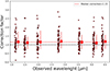 |
Fig. A.1. The correction factor versus observed wavelength for the sample of C III] emitters. The median correction of 1.15 is shown by the dashed red line |
On average, there is a slit-loss factor of around 1.1-1.2, and it is wavelength-independent i.e. on average, we find the same correction factor across all filters although the scatter is large. For the galaxies where we find an average correction factor > 1 (33 sources in total), the correction is made by multiplying the flux densities of the spectrum by the average factor for each galaxy. For galaxies with an average correction factor < 1, no correction is applied (meaning a correction factor = 1 is assumed) because in those cases there are no slit-losses.
Appendix B: The O III] / He II ratio
To obtain a reliable measure of the He II that we employ in the UV diagnostic diagrams, we calculate the O III] / He II line ratio from stacked spectra of our C III] emitters. Following the methodology described in Sec. 3, we stacked the spectra of the entire sample of selected C III] emitters. Due to the low-resolution of the prism spectrum, the two lines are blended. However, the high SN of the stack allows up to model the two components separately and infer their relative contribution to the blend. For the modeling, we assumed two blended Gaussian components with fixed central wavelength for each line and a local continuum. In the top panel of Fig. B.1 we show the results of the Gaussian modeling and the continuum-subtracted stacked spectra: clearly two Gaussians can fit the line blend much better than one component alone. We measure a ratio of 0.87±0.38 in the entire stack of C III] emitters and we thus apply this value to individual emitting galaxies. We repeated the exercise for stack of the non-C III] emitters and the ratio derived is slightly higher but still well within the uncertainty. As shown in bottom panel in Fig. B.1, these empirically derived values fall within the range observed for SFGs in the VANDELS survey, showing particular consistency with the most extreme C III] emitters (EW ∼5–10 Å) in that sample. Furthermore, the ratio ares consistent with the value derived from the stack presented in Amorín et al. (2017), which itself occupies the AGN region of standard UV diagnostic diagrams. Finally very similar O III] / He II ratios are found when stacking galaxies at z ∼ 5.6 − 9 using NIRSpec medium resolution spectra (Hu et al. 2024).
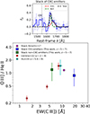 |
Fig. B.1. Top panel: continuum-subtracted stacked spectrum of C III] in the sample (blue line) and the corresponding uncertainty (blue shaded region). The dashed red and green lines represent the best-Gaussian fit of O III] and He II, respectively, while the dashed black line represents the total fit of the blend lines. The vertical gray line indicates the position of C IV. Bottom panel: the O III] / He II line ratio as a function of C III] equivalent width. The blue square represents the O III] / He II ratio measured in the stack, yielding a value of 0.87±0.38. This value is compared to measurements from Amorín et al. (2017), Llerena et al. (2022) and Hu et al. (2024). |
Appendix C: Properties of the C III] emitters sample
In Table C.1, we present the properties of the C III] emitter sample, including coordinates, redshift, and the results of our AGN diagnostics. It also includes the EW values and the UV β slopes.
Properties of the C III] emitter sample
Table C.2 shows the values of the line ratios and EWs used for our three stacks.
UV and optical emission-line ratios and equivalent widths for stacked samples.
All Tables
UV and optical emission-line ratios and equivalent widths for stacked samples.
All Figures
|
Fig. 1. Rest-frame spectra of C III]-emitters from different surveys. Both panels show the rest-frame wavelength in Ångströms on the x axis and flux density in units of 10−21 erg s−1 cm−2 Å−1 on the y axis. |
| In the text | |
|
Fig. 2. Redshift distribution of the galaxy sample. The histogram shows the number of galaxies as a function of redshift between z = 5 and z = 7, with a pronounced peak at z = 5.25. |
| In the text | |
|
Fig. 3. Rest-frame C III] EW (in Å) versus absolute UV magnitude (MUV; AB mag). Blue points show the sample of C III] emitters at z = 5 − 7. Red points show the VANDELS sample compiled by Cunningham et al. (2024) at z = 3 − 4. Contour plots and linear regression fits are also shown. |
| In the text | |
|
Fig. 4. Star formation rate (SFR) versus stellar mass from our sample compared to the star formation of field galaxies at z = 5 − 7. Our sample is colour-coded by the rest-frame C III] EW. The general parent population in the same redshift range appears as grey circles. The blue line represents the relationship found by Calabrò et al. (2024), derived with SFR based on Hα for a similar spectroscopic sample. |
| In the text | |
|
Fig. 5. Stacked spectra for non-C III] emitters (top panel), weak (middle panel), and strong (bottom panel) C III] emitters. In all panels, the shaded regions represent the 1σ uncertainty of the stacking. The dashed vertical black line indicates the position of the rest-frame UV emission lines. |
| In the text | |
|
Fig. 6. Example of a galaxy with a significant broad Hα component: GDS-13704 at z = 5.93. The black line shows the observed spectrum. The blue line represents the best-fit model using a double Gaussian profile. The red line shows the narrow component, while the green line corresponds to the broad component. The x axis shows the rest-frame wavelength in Angstroms, and the y axis shows the flux density in units of 10−21 erg s−1 cm−2 Å−1. This source has a ΔBIC = 34.5, providing strong evidence for the presence of broad-line emission. |
| In the text | |
|
Fig. 7. Black hole mass versus stellar mass. Blue stars show our nine C III] emitters with broad Hα emission, compared with 4 < z < 10 AGNs (grey squares; Harikane et al. 2023; Kocevski et al. 2023; Juodžbalis et al. 2026; Wang et al. 2024; Übler et al. 2024; Akins et al. 2025; Kokorev et al. 2023; Larson et al. 2023; Bogdán et al. 2024; Maiolino et al. 2024, full references in the text), a compilation of 2 < z < 7 QSOs (grey cross; treated as upper limits; Tripodi et al. 2024, see references therein), and local scaling relations (dashed grey, solid red and dotted yellow lines, respectively from refs. Kormendy & Ho 2013; Reines & Volonteri 2015; Greene et al. 2020). |
| In the text | |
|
Fig. 8. UV-diagnostic diagram showing the EW of C III] versus the ratio C III]/He II. The SFG and AGN models are from Nakajima & Maiolino (2022), while the dashed black line is from Nakajima et al. (2018). Values measured from the stacked spectra are shown as purple (weak stack), light green (strong stack), and pink (no C III] stack) points, with lower-redshift stacks (darker green) from Llerena et al. (2022). The C III] emitters with a broad Hα are plotted as red diamonds. Four galaxies that lie outside the range of the plot and have upper limits on He II emission are GDS-5093, RUBIES-49140, CAPERS-101195, and CAPERS-9244, with C III]/He II values of 0.04, 0.09, 0.02, and 0.01, respectively; the EWs of C III] are listed in Table C.1. |
| In the text | |
|
Fig. 9. UV-diagnostic diagram showing the EW of C IV versus the ratio C IV/He II. The demarcation lines are given by Hirschmann et al. (2019). Models and stacks are the same as in Figure 8. |
| In the text | |
|
Fig. 10. Star-forming galaxy (SFG) models from Gutkin et al. (2016) and AGN models from Plat et al. (in prep.) in the OHNO diagram. The dashed black demarcation line is from Feuillet et al. (2024), while the solid black line is from Arevalo-Gonzalez et al. (2025). Stacked measurements are shown as purple (weak stack), light green (strong stack), and pink (no C III] stack) points. The C III] emitters with a broad Hα are plotted as red diamonds. The values for RUBIES-15072 (outside the plot range) are log10([Ne III] λ3869/[O II] λλ3726,3279) = 2.22 and log10([O III]/Hβ) = 0.83 ± 0.08. |
| In the text | |
|
Fig. 11. Rest-frame spectra of the five little red dots identified in our sample. From left to right, top to bottom: COSMOS-61234, CAPERS-35805, RUBIES-49140, GDS-13704, and UNCOVER-41225. |
| In the text | |
|
Fig. A.1. The correction factor versus observed wavelength for the sample of C III] emitters. The median correction of 1.15 is shown by the dashed red line |
| In the text | |
|
Fig. B.1. Top panel: continuum-subtracted stacked spectrum of C III] in the sample (blue line) and the corresponding uncertainty (blue shaded region). The dashed red and green lines represent the best-Gaussian fit of O III] and He II, respectively, while the dashed black line represents the total fit of the blend lines. The vertical gray line indicates the position of C IV. Bottom panel: the O III] / He II line ratio as a function of C III] equivalent width. The blue square represents the O III] / He II ratio measured in the stack, yielding a value of 0.87±0.38. This value is compared to measurements from Amorín et al. (2017), Llerena et al. (2022) and Hu et al. (2024). |
| In the text | |
Current usage metrics show cumulative count of Article Views (full-text article views including HTML views, PDF and ePub downloads, according to the available data) and Abstracts Views on Vision4Press platform.
Data correspond to usage on the plateform after 2015. The current usage metrics is available 48-96 hours after online publication and is updated daily on week days.
Initial download of the metrics may take a while.