| Issue |
A&A
Volume 709, May 2026
|
|
|---|---|---|
| Article Number | A34 | |
| Number of page(s) | 9 | |
| Section | The Sun and the Heliosphere | |
| DOI | https://doi.org/10.1051/0004-6361/202558124 | |
| Published online | 01 May 2026 | |
Signatures of localised particle acceleration at a global coronal shock wave
1
Centre for Astrophysics and Relativity, School of Physical Sciences, Dublin City University, Glasnevin Campus, Dublin D09 V209, Ireland
2
Astronomy & Astrophysics Section, School of Cosmic Physics, Dublin Institute for Advanced Studies, DIAS Dunsink Observatory, Dublin D15 XR2R, Ireland
3
LIRA, Observatoire de Paris, PSL Research University, CNRS, Sorbonne Université, Université Paris Cité, 5 place Jules Janssen, 92195 Meudon, France
★ Corresponding author: This email address is being protected from spambots. You need JavaScript enabled to view it.
Received:
14
November
2025
Accepted:
19
March
2026
Abstract
Context. Extreme ultraviolet (EUV) waves are global waves in the solar corona that accelerate particles. The efficiency of this acceleration depends on local plasma characteristics such as the Alfvén speed and the geometry of the magnetic field. This shock-driven particle acceleration produces radio signatures such as Type II radio bursts and herringbone emission.
Aims. Here we investigate signatures of particle acceleration by a weak coronal shock on 10 March 2024. In particular, we combined EUV images with radio imaging and spectral observations to determine how and where this weak shock could accelerate energetic particles.
Methods. A potential field source surface extrapolation was used to examine the pre-eruption ambient magnetic field, while the evolution of the global wave was probed using running-difference and base-difference EUV images. The EUV images enabled the speed and Alfvèn Mach number of the EUV wave to be characterised. The combination of radio images and dynamic spectra provides evidence of beams of shock-accelerated electrons localised to a dimming region at the time the EUV wave passes through it. The speeds and energies of these electrons were estimated from the drift rates of their herringbones.
Results. The EUV wave initially propagated due west, channelled by two large loop systems, before changing direction northwards. From the EUV intensity jump at the wavefront, the Alfvén Mach number was estimated to be approximately 1.005 at the time the herringbones were produced. The herringbone drift rates reveal accelerated electron energies of 75.32 to 122.10 keV, using Newkirk density models with scaling factors of 1.3 to 2.6.
Conclusions. These observations suggest that the weak lateral shock impacted a quasi-perpendicular open field in a dimming region, enabling localised particle acceleration. This indicates that the geometry of the ambient magnetic field relative to the shock strongly governs where particles are accelerated.
Key words: Sun: corona / Sun: coronal mass ejections (CMEs) / Sun: particle emission / Sun: radio radiation
© The Authors 2026
 Open Access article, published by EDP Sciences, under the terms of the Creative Commons Attribution License (https://creativecommons.org/licenses/by/4.0), which permits unrestricted use, distribution, and reproduction in any medium, provided the original work is properly cited.
This article is published in open access under the Subscribe to Open model. This email address is being protected from spambots. You need JavaScript enabled to view it. to support open access publication.
1. Introduction
Uchida (1968) proposed the existence of coronal fast mode magnetohydrodynamic waves as the cause of Moreton-Ramsey waves, chromospheric bright fronts in H-alpha images, first observed by Moreton (1960), Moreton & Ramsey (1960). Uchida suggested that Moreton-Ramsey waves were the footprints of coronal waves interacting with the chromosphere, in order to explain their observed high speeds (500–1500 km s−1), which were incompatible with wave propagation directly through the chromosphere but consistent with estimated coronal fast-mode speeds. Globally propagating waves in the solar corona were first observed by the Extreme ultra-violet Imaging Telescope (EIT; Delaboudinière et al. 1995) on board the Solar and Heliospheric Observatory (SOHO) in 1997 (Thompson et al. 1998; Dere & Brueckner 1998). They were observed as a bright circular wavefront propagating out from an active region, across the disk, at a height of approximately 70–90 Mm above the photosphere (cf. Patsourakos et al. 2009). Biesecker et al. (2002) found that these extreme ultra-violet (EUV) waves are always accompanied by a coronal mass ejection (CME), but not every CME has an associated EUV wave. From initial studies based on EIT observations, the speeds of EUV waves were found to be typically in the range of 200–400 km s−1 (Thompson & Myers 2009), much lower than measured Moreton-Ramsey wave speeds and expected coronal fast mode wave speeds.
Due to this apparent discrepancy, other theories arose to explain EUV waves, with some describing these phenomena as slow-mode solitons (Wills-Davey et al. 2007), and some describing them as pseudo-waves. Theories in the pseudo-wave branch postulate that these brightenings arise from field line stretching (Chen et al. 2002), Joule heating in current shells (Delannée et al. 2007), or continuous small-scale reconnection (Attrill et al. 2007). After the launch of Solar Dynamics Observatory (SDO; Pesnell et al. 2012), its EUV imager, Atmospheric Imaging Assembly (AIA; Lemen et al. 2012), enabled high cadence imaging of the solar corona, with a time resolution of 12 s in comparison with EIT’s time resolution of 720 s. Studies of EUV waves imaged with AIA have yielded much higher EUV wave speeds than previous work. Nitta et al. (2013) show that EUV wave speeds span a broad range of approximately 200–1500 km s−1, with mean and median values around 600 km s−1. These speeds, along with results from differential emission measure analysis (Vanninathan et al. 2015) and simulations (Downs et al. 2012, 2021), and observations of co-spatial radio sources (cf. Carley et al. 2013; Morosan et al. 2019) support the interpretation of EUV waves as brightenings due to heating and compression at fast-mode magnetohydrodynamic wave or shock fronts, driven by the associated expanding CME. As a result, growing general consensus favours interpreting EUV waves as fast-mode waves or shocks (Long et al. 2017).
Radio sources at the EUV wavefront reveal locations and times where the wave exceeds the local fast-mode speed, becoming a shock and accelerating particles (cf. Morosan et al. 2019). Combining this with radio spectra, we can estimate the height at which electrons were accelerated by the shock, and their resultant energy. Charged particles are accelerated by shocks via shock drift acceleration and diffusive shock acceleration (Holman & Pesses 1983; Street et al. 1994). Despite typically being subcritical (Long et al. 2021), coronal shocks have been shown to accelerate particles (Rouillard et al. 2012; Prise et al. 2014), suggesting that even weak shocks can accelerate particles in coronal conditions. Scattering and turbulence in the corona play an important role, especially in the case of diffusive shock acceleration, where the energy gained by a particle in a single crossing of the shock is very small, but after many repeated crossings, the particle can become highly accelerated (Ball & Melrose 2001; Carley et al. 2013). Shocks become efficient at energising electrons via shock drift acceleration in regions where the magnetic field is quasi-perpendicular to the shock normal, as electron motion is confined along the shock (Carley et al. 2013; Maguire et al. 2020). Long et al. (2021) attributed electron acceleration by a weak shock to interaction between the shock and the ambient magnetic field.
Type II and type III radio bursts are signatures of accelerated electrons in the corona (Nelson et al. 1985; Reid 2020). When electrons are accelerated in coronal plasma either by shocks or magnetic reconnection, this non-thermal population of electrons causes electrostatic plasma oscillations called Langmuir waves. These oscillations can combine with ion acoustic waves, producing electromagnetic waves at the fundamental frequency of the plasma. Two Langmuir waves can alternatively coalesce to produce electromagnetic waves at the second harmonic of the plasma frequency. The fundamental plasma frequency is proportional to the square root of the electron number density. At the density range of the corona, the range of fundamental and harmonic plasma frequencies are in the range of tens to hundreds of megahertz.
Type III radio bursts are short-lived radio bursts with a large negative drift rate (typically df/dt ≈ −100 MHz s−1; Reid & Ratcliffe 2014). They represent plasma emission at rapidly decreasing frequency due to a beam of energetic electrons escaping on open magnetic field lines. They are regularly observed from active regions during flares, in which case they signify the escape of electrons accelerated by magnetic reconnection (Reid & Ratcliffe 2014; Reid 2020). Type III bursts have also been observed near the location of a shock front, as inferred from an observed EUV wave in Long et al. (2021). In this case the emission indicates the escape of shock-accelerated electrons. Type II radio bursts are longer-lived radio bursts with lower drift rates (typically df/dt ≈ 0.1 MHz s−1 (Mann et al. 1996)). They occur due to shock acceleration of electrons as a shock travels outwards and passes through plasma of progressively lower electron density. Type II radio bursts have also been imaged at EUV wavefronts (cf. Mancuso et al. 2021).
Herringbones are a fine structure present in type II bursts (Mann & Klassen 2005). They appear above and/or below the type II on a dynamic spectrum, with those extending to lower frequencies having a forward drift and those extending to higher frequencies having a reverse drift. They are caused by shock-accelerated electrons travelling on magnetic field lines, either out into interplanetary space (forward drift) or down deeper into the lower corona (reverse drift). Radio imaging of herringbone radio emission has confirmed that they originate from shocked regions (Morosan et al. 2019).
In this paper, we combine observations of an EUV wave from SDO/AIA with spectral observations of a type II radio burst and herringbones from the Radiospectrographic Observations for FEDOME and the Study of Solar Eruptions (ORFEES; Hamini et al. 2021) and the Compound Astronomical Low frequency Low cost Instrument for Spectroscopy and Transportable Observatory (CALLISTO; Benz et al. 2005), along with radio images from the Nançay RadioHeliograph (NRH; Mercier et al. 1988). We present rare imaging observations of herringbones, which interestingly appear at the EUV wavefront as it interacts with a transient dimming region. From our analysis of the AIA images, we find that the shock responsible for particle acceleration at this location is very weak. Our findings suggest that the interaction between the shock and the local magnetic field is a crucial factor in enabling the shock acceleration of electrons in this event. This is in agreement with the findings of Long et al. (2021). In Sect. 2 we detail the observational data utilised in this study. In Sect. 3 we describe our methods and results, and in Sect. 4 we provide further discussion and conclusions.
2. Observations
On 10 March 2024, a Geostationary Operational Environmental Satellite (GOES) M7.4-class X-ray flare was detected from Active Region (AR)13599, between 12:00 UT and 12:20 UT, peaking at 12:08:54UT. The associated CME reached the base of the LASCO C2 field of view (2.5 R⊙) at 12:36 UT, with a central position angle of 275° counter-clockwise from north, and a velocity of 307 km s−1. Images from AIA show remote brightening in AR13602 at the time of the flare, indicating that this active region is magnetically connected to the flare site. AIA running-difference images depict an EUV wave propagating out from AR13599 between 12:09:33 UT and 12:19:33 UT. AIA base difference images in 211 Å and 193 Å exhibit dimming in the remote but connected region, AR13602, following the flare. The CME’s position angle and velocity, as measured by LASCO, together with the timing of the dimming, the EUV wave, and the CME’s arrival at the base of the LASCO C2 images, support the interpretation that the EUV wave is produced by the expanding CME in the low corona and that the dimming in AR13602 results from the loss of material to the expanding CME. Dynamic spectra from ORFEES and CALLISTO reveal a type II radio burst with many reverse herringbones. Some of the herringbones were also observed spatially by NRH. No forward-drifting herringbones can be seen; however, this may be due to poorer resolution at lower frequencies.
2.1. EUV observations
We followed the recommended processing steps for AIA images, utilising tools from the aiapy.calibrate sub-package. For each AIA map used in our analysis, we applied the update_pointing function to update the image metadata describing satellite pointing. We then applied the register function, which upgrades AIA images from level 1 to level 1.5, by removing the roll angle, aligning the centre of the image with the centre of the Sun and scaling the image to a common resolution across the channels. Lastly, we normalised each map by dividing each map by its exposure time. We also removed images with exposure times below a threshold of 1.5 s from our dataset, noting a relatively small number of images with an exposure time less than 1.5 s; these images had noticeably lower intensities than the others.
AIA captured an EUV wave, visible in the 211 Å running-difference images between 12:09:33 UT and 12:19:33UT. The angular extent and direction of propagation can be seen in the right-hand panel of Fig. 1 and in the accompanying online in the online version. Although the wave initially appears to travel westwards, at approx. 12:10:45 UT the bubble appears to gain a stronger northward component. Base ratio images reveal that AR13602, to the north of the flaring active region, dims as the EUV wave begins to propagate northwards.
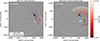 |
Fig. 1. AIA 211 Å running difference images from 12:11:09 UT on 10 March 2024. Left: Paths used for tracking the EUV wave plotted on an AIA 211 Å running-difference image offset by 1 minute. Right: Manually identified leading-edge fronts for 27 running-difference images (12:09:33–12:19:33 UT) overplotted on the 12:11:09 UT image. Each front is shown in a unique shade of red to indicate its timing. The online version provides this information in a online. |
2.2. Radio observations
Between 12:11 and 12:18 UTC, a type II radio burst with herringbones was observed by the CALLISTO solar spectrometer stations in Greenland and Algeria, as well as the ORFEES radio spectrograph in Nançay, France (see Fig. 2). The extended CALLISTO network, e-CALLISTO, includes stations across the world, ensuring that at least one instrument observes the Sun almost 24 hours a day. The total frequency of CALLISTO ranges from 45 to 870 MHz, and it has a time resolution of 0.25 sec. The integration time is 1 ms, and the radiometric bandwidth is about 300 KHz (Benz et al. 2005). ORFEES observes the whole-Sun flux density between 144 and 1004 MHz, which corresponds to regions between the low corona and half a solar radius above the photosphere (Hamini et al. 2021). Combining radio spectrogram data from ORFEES, CALLISTO Algeria, and CALLISTO Greenland, we see the type II radio burst from approximately 150 to 50 MHz and its reverse herringbones from approximately 150 to 270 MHz (see Figs. 2a and b). When plotting dynamic spectra, we performed background normalisation to remove the background response.
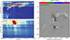 |
Fig. 2. (a): Type II radio burst seen in the dynamic spectra, captured between approximately 240 and 40 MHz from approximately 12:11:30 UT to 12:20:45 UT by ORFEES and CALLISTO in Greenland and Algeria. The colour map used in this dynamic spectrum is not representative of the actual relative intensities; it was normalised differently across the two datasets to highlight the type II feature for the reader. (b): Zoom-in on ORFEES herringbones between 12:13:00 UT and 12:13:20 UT. The points identifying one of these herringbones are shown at frequencies corresponding to the NRH contours on the right (black crosses, dashed black connecting line). (c): 211 Å running-difference image from 12:13:09 UT with NRH contours over-plotted between 150.9 MHz and 270.6 MHz. The EUV wave has just passed over the open field region, and reverse herringbone emission has been triggered. The plotted contours show the path of the identified herringbone. The online version provides this information in a online. |
The NRH captured image data during the event at ten frequencies between 150.9 and 444 MHz, with a cadence of 0.25 s. We used SolarSoftWare (SSW) to process the NRH data (Freeland & Handy 1998). This involved cleaning the data with default parameter settings and computing images. Imaging of sources at 150.9 to 270.6 MHz shows that the herringbone electron beams are localised to a specific region in the EUV wave’s path, and that they are triggered by the arrival of the wave.
3. Methods and results
3.1. EUV analysis
To characterise the global wave, we produced 211 Å running-difference images, with an offset of 1 minute. From these images, we identify the angular expanse of the EUV wave to be from about –45° to 135°, defining 0°as west of the NOAA Active Region 13599, at a helioprojective latitude of –125″and a helioprojective longitude of 606″. Paths starting at this point were picked at 10° intervals in this chosen angular range, using great arcs in the region where θ > 85°and straight radial lines for all θ ≤ 85°. This delimits the sector of the wave’s path that remains predominantly on-disk within the field of view from the sector that extends significantly off-disk. On-disk, we tracked the wave along the curved surface of the Sun. Off-disk, we tracked it in the plane of sky. The left panel of Fig. 1 shows these paths plotted on the AIA 211 Å running-difference image for 12:11:09UT. For each path, we created a distance versus time stack-plot by extracting the pixel intensities along the path for each frame over the duration of the EUV wave. Our method was similar to that used in Francile et al. (2016). These stack-plots can be seen in Fig. 3. The bright feature in a distance versus time stack-plot has a slope that corresponds to the wave speed along the direction of the path. We visually identified points along the bright feature of the intensity stack-plots. We used linear fitting to find the wave speed along each of the chosen paths. We found a mean velocity of 1029 ± 45 km s−1. We also used quadratic fits to estimate any acceleration of the wave and found little to no acceleration, with a mean value of –3.6 ± 2.5 km s−1. For paths that passed through the dimming region, i.e. those labelled 115 to 135°, we found a mean velocity of 798 ± 73 km s−1.
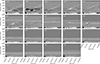 |
Fig. 3. Stack-plots for each path, shown in the left hand side of Fig. 1 organised by decreasing angle (top left to bottom right). The stack-plots in the top row correspond to those along great arc paths, and the others correspond to those along straight line paths. The horizontal white line denotes the distance from AR13599 to the limb along the relevant path. For each frame where the wave is visible along the path in question, the distance from the AR of the nearest clicked point to the path is shown in red. |
In addition to the stack-plot technique, we also employed a point-and-click method to visually identify the leading edge of the EUV wave in each running-difference image. The EUV wave was visible in our 211 Å running-difference images between 12:09:33 UT and 12:19:33UT. For each of these images, points on the leading edge of the EUV wave were first manually identified, then joined to draw a wavefront. In the right panel of Fig. 1, all of these manually estimated wavefronts are plotted on a 211 Å running-difference image from 12:11:09UT. In the online version, we present this in online form. The EUV brightening is fainter at later times, when the wave is furthest from the active region source. Therefore, in these later frames, it is more difficult to pinpoint the leading edge. Along the longest paths, the stack-plots also become faint far from the source. To compare the leading edge of the brightening detected in the running-difference images and stack-plots, we over-plotted the clicked points closest to the paths in each frame onto the stack-plots, as shown in Fig. 3.
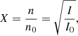
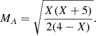
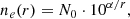
We estimated the Alfvén Mach number, MA, of the global wave as it passed through the dimming region and produced herringbones. We used the approach of Zhukov (2011) to estimate the density compression ratio X, from the observed 193 Å intensity enhancement I/I0, using the following relation:
 (1)
(1)
where I0 is the mean background intensity and I is the peak intensity during the passing of the wave. As further discussed by Zhukov (2011), the assumption I ∝ ne2 is most appropriate for a passband whose temperature response is dominated by Fe XII emission formed at ∼1.4 MK, making the 193 Å AIA passband the most suitable for this analysis. To calculate MA from X, we used the equation below from Vršnak et al. (2002):
![Mathematical equation: $$ \begin{aligned}&(M_A - X)^2\left(5\beta X + 2M_A^2 \cos ^2\theta (X - 4)\right) \nonumber \\&\quad + M_A^2 X \sin ^2\theta \left[(5 + X)M_A^2 + 2X(X - 4)\right] = 0, \end{aligned} $$](/articles/aa/full_html/2026/05/aa58124-25/aa58124-25-eq2.gif) (2)
(2)
where plasma β is the ratio of the thermal plasma pressure to the magnetic field pressure and θ is the angle between the shock normal and the magnetic field. For a parallel shock (θ = 0°), Eq. (2) becomes
 (3)
(3)
and for a perpendicular shock (θ = 90°):
 (4)
(4)
We did not directly calculate the Alfvén Mach number of the dimmed region as the dimming caused fluctuations in intensity, which would have caused a high degree of uncertainty in the background intensity and the resultant Mach number. To estimate the Mach number of the wave passing through the dimmed region, we chose a region in the quiet corona that the wave passed through at approximately the same time as it passed through the dimmed region. We found the mean intensity ratio in the region, comparing its peak frame to a background frame. We calculated the resulting Alfvén Mach number both for the parallel and perpendicular shock configurations, finding MA = 1.004 ± 0.002 for a parallel magnetic field and MA = 1.006 ± 0.003 for a perpendicular magnetic field. These uncertainties propagate from the standard error of the intensity ratio in the region, as we considered this to be the largest source of uncertainty.
To quantify the level of dimming in AR13602 at the time of the main herringbone emission in this region (12:13:00 to 12:13:20 UT), we produced base-difference ratio images from AIA 211 Å images, using a pre-flare base image from 12:08:45UT. The pixel intensities of a base-difference ratio image, Ibdr, are
 (5)
(5)
where I0 is the pixel intensity in the base image and I is the pixel intensity in the current image. We examined the time profile of mean pixel values of the base-difference ratio images and found that at the time of interest, the mean intensity of the dimming region had dropped by approximately 45% of its base-level intensity. For more detail see Fig. 4. As detailed in Robbrecht & Wang (2010), dimming in coronal pass bands occur due to a decrease in plasma density or a change in plasma temperature. From base-difference images, we identified simultaneous dimming in AR13602 in the 211 Å, 193 Å, and 171 Å passbands and from running-difference images we did not identify any enhancement in 94 Å. This combination of multi-channel dimming and the absence of heating signatures disfavours a thermal interpretation and favours density depletion due to plasma evacuation. Scaled Newkirk models with fold numbers between 2 and 4 are routinely used to approximate the radial density profile of active regions (e.g. Vasanth et al. 2014; Mann et al. 2018; Bhunia et al. 2025). Attributing the dimming of this active region by 45% to a decrease in density, we applied a Newkirk density model with scaling factors of 1.3-2.6 to approximate the region’s density profile.
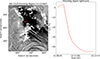 |
Fig. 4. Left: 211 Å base-difference ratio image of the area surrounding AR13602, at 12:13:09UT, using a quiet-time base frame from 12:08:45UT. The red box indicates the subregion, which the light curve on the right corresponds to. This subregion was identified as remaining within the dimming region throughout the period when dimming occurred. Right: Base-difference ratio light curve for the subregion, dimming by up to 45.77%. |
We also estimated the Alfvèn Mach number with a second method for comparison. We first estimated the Alfvèn speed in the dimming region based on typical active region values, then calculated the Mach number as the ratio of the speed of the wave in this area (798 km s−1) to the Alfvèn speed. Assuming a height of 1.1 R⊙ (approximately the typical height of coronal waves (cf. Patsourakos & Vourlidas 2009) and adopting a coronal magnetic field strength of 10 G, consistent with empirical active region coronal field models presented in Gary & Alexander (1999), together with a 1.3 fold Newkirk density model, we calculate an Alfvèn speed of 900 km s−1 and therefore a Mach number of 0.89. If we use a 2.6 fold Newkirk model, we find an Alfvèn speed of 637 km s−1 and thus an Alfvèn Mach number of 1.25.
3.2. Radio analysis
For each NRH frequency, we over-plotted the 80 and 90% contours on the AIA 211 Å running-difference images and collated these in a online, with the dynamic spectra from ORFEES and CALLISTO for the same time window displayed along side it. From the online we noticed the following. A group of reverse drifting herringbones from 12:11:12 UT to 12:11:20 UT appears to be triggered at the southern edge of the dimming region, AR13602, predominantly between 150.9 and 228.0 MHz. This coincides with the arrival of the EUV wave in this region. At 12:12:27 UT the dimmed region again becomes the main source of 150.9 – 173.2 MHz radio emission. Between 12:12:27 UT and 12:14:13 UT, this source moves along with the EUV wave, at times extending to 228.0 MHz. This implies that the emission is due to accelerated particles at the shock front. At 12:13:05 UT the 270.6 MHz contours become aligned with this source.
We identified sixteen reverse herringbones in the ORFEES dynamic spectrum between 12:13:00 UT and 12:13:20 UT, drifting from approximately 150 MHz to approximately 270 MHz. The NRH images reveal that this emission is localised to the dimmed region. Figure 2 highlights one herringbone in the dynamic spectra and shows its closest NRH contours over-plotted on an AIA 211 Å running-difference image. For each of the sixteen herringbones, we identified the frequency–time points on each herringbone that matched the four NRH imaging channels: 150.9, 173.2, 228.0, and 270.6 MHz. Figure 5 shows the position in time of the herringbone electron beams, at the heights corresponding to the four channels.
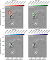 |
Fig. 5. Top left to bottom right: NRH contours corresponding to herringbone emission between 12:13:00 UT and 12:13:20 UT at 150.9 MHz, 173.2 MHz, 228.0 MHz, and 270.6 MHz, over-plotted on the 211 Å running-difference image for 12:15:09UTC. Sixteen contours corresponding to sixteen herringbones are shown for 150.9 MHz and 173.2 MHz. Bottom left: Fifteen contours for fifteen herringbones extending to 228.0 MHz. Bottom right: Eight contours shown for eight herringbones extending to 270.6 MHz. |
Herringbones have been approximated by straight lines in previous studies, (e.g. Carley et al. 2015; Zhang et al. 2024). The herringbones in this event had steepening drift rates that were better approximated by quadratic curves than straight lines. Using Eq. (8) and scaled Newkirk density models to relate fp to a corresponding radius, these drift rates imply radial beam speeds that increase as the electrons travel deeper into the corona. This results from electrons travelling downwards along curved magnetic field lines. The speed of these particles does not in fact increase as they travel downwards, but the radial component of their velocity increases as the field lines they travel on become more purely radial lower down.
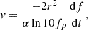
Given the relationship between plasma density (ne) and plasma frequency (fp),  , coronal electron density models allow us to estimate the height of radio emission based on its frequency, assuming that it is either fundamental emission (f = fp) or harmonic emission (f = 2fp). The frequency drift of herringbones indicates the propagation of the beam through areas of changing density. Assuming that this change in density corresponds to a change in coronal height in accordance with a density model, ne(r), we can infer the speed of the beam from the drift rate (df/dt) using the following expression (Morosan et al. 2019):
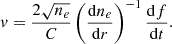 (6)
(6)
Using a Newkirk (1961) density model of the form,
 (7)
(7)
Eq. (6) becomes
 (8)
(8)
where r is chosen to be the starting height of the herringbone and fp is chosen to be the starting frequency.
For each of the sixteen herringbones, we identified twenty points and fitted a quadratic curve to those points. Differentiating frequency as a quadratic function of time, we found drift rate as a linear function of time for each burst, then used Eq. (8) to estimate the electron beam velocity as a function of time. We find that the herringbones had starting frequencies of approximately 150 MHz and drift rates ranging from +45 MH z−1 to +85 MH z−1. The Newkirk (1961) model (i.e. Eq. (7) with N0 = 4.2 × 10⁴, α = 4.32) approximates the electron density in the corona from 1–3 R⊙, with different fold numbers depending on the activity of the region. We found upper and lower limits for the herringbone electron speeds and starting heights, based on scaling factors of 1.3 to 2.6. Given this range of scaling factors, if we assume that the radio emission is fundamental, the electron beams have a starting height in the range of 1.16 to 1.27 R⊙ and have mean velocities of 0.18 to 0.21 c, corresponding to mean kinetic energies of 8.02 to 11.67 keV. If the emission is assumed to be harmonic, using the same range of scaling factors, we get a starting height in the range of 1.39 to 1.54 R⊙, downward velocities of 0.49 to 0.59 c, and kinetic energies of 75.32 to 122.10 keV.
3.3. Magnetic field
We modelled the pre-eruption coronal magnetic field by performing a potential field source surface extrapolation with the sunkit-magex.pfss Sunpy module (Stansby et al. 2020), using the Global Oscillation Network Group (GONG) magnetogram synoptic map observations from 12:04:00 UT. Figure 6 shows the potential field source surface (PFSS) field lines overplotted on the closest AIA 193 Å image at 12:04:04 UT. For the PFSS extrapolation, we made a grid of 20-by-20 seed footpoints in the range –85° to 85° latitude and 0° to 85° longitude, at a height of 1.15 R⊙. The apparent extension of field lines beyond this region in Fig. 5 arises because field lines traced from these seeds may map to different locations outside these bounds. We chose these ranges as the EUV wave is only visible propagating across the western half of the disk, and we wanted to avoid the polar regions, where uncertainties in the extrapolated field become very large.
 |
Fig. 6. PFSS magnetic field extrapolation just before the flare. The field lines are plotted on an AIA 193 Å image. The closed field lines are in white, and the open field lines are in cyan. The location of the herringbone contours in AR13602 is as indicated. The yellow arrows highlight the large loop systems to the north and south of the flaring active region, which is marked by the ‘AR’ label. |
Figure 6 shows a large loop system to the east and south of AR13599, and another to the north of the active region, connecting AR13599 to AR13602. These loops indicate regions of strong, closed magnetic fields in the low corona. Such regions have higher Alfvèn speeds, reducing the Alfvèn Mach number of the wave and diminishing its ability to compress and heat plasma. This caused the bright front to initially propagate preferentially towards the west. The gap between the two loop systems is approximately the expanse of the EUV wave in the first few frames of our 211 Å running-difference online, as seen in the right panel of Fig. 1. Coronal dimming in AR13602, apparent in the 211 Å base-difference images, suggests that material flows out from the region into the heliosphere, leaving behind an area of open magnetic field. Due to this change in the configuration of the magnetic field, the EUV wave then propagates in a more northerly direction.
4. Discussion and conclusions
In this paper, we presented observational evidence of localised particle acceleration by a weak, subcritical coronal shock associated with the 10 March 2024 eruption. This event provides a useful set of observations to study the conditions in which a weak plasma shock can give rise to particle acceleration.
By analysing AIA images, and modelling the pre-eruption coronal magnetic field, we examined the propagation path of the wave and the coronal conditions it encountered. We found that during the passage of the wave, there was an outflow of plasma from a connected active region, which was related to a reconfiguration of the magnetic field. This allowed the EUV wave, which initially travelled approximately due west, to gain a more northward component. The EUV wave then propagated into the region from which material had been lost, where it encountered open magnetic field lines, quasi-perpendicular to its path. A full understanding of the trajectory of the EUV wave and the evolution of the erupting flux rope, which was not directly observable, would require dedicated magnetohydrodynamic modelling of the eruption and its interaction with the surrounding coronal magnetic field.
The type II radio burst and reverse drifting herringbones seen in the dynamic spectra indicate acceleration of particles by a shock. Radio images from NRH confirm that this particle acceleration occurs at the open field region, when the EUV wave impacts it. We checked the location of each radio contour for sixteen herringbones, at the four relevant NRH frequency channels, finding that these electron beams were undoubtedly localised in the north-east of the dimming region and that they were temporally confined to the window when the EUV wave passed through this region (Fig. 5).
The combined radio and EUV observations indicate that the wave encounters conditions favourable for shock particle acceleration when it reaches the remaining open field lines in the dimmed region. From the increase in 193 Å intensity at the EUV wavefront, we estimate an Alfvèn Mach number of MA ≈ 1.004 − 1.006 depending on the angle between the ambient magnetic field lines and the shock normal. These values are within the range of Alfvèn Mach numbers, calculated based on the speed of the EUV wave through the dimmed region (798 km s−1) and typical Alfvèn speeds, considering that the dimming region is also an active region. Assuming a height of 1.1 R⊙ and a magnetic field strength of 10 G (Gary & Alexander 1999) and approximating the electron density using a 1.3–2.6× Newkirk density model, we find a broader range of MA ≈ 0.89 − 1.25. This is a rough estimate due to our assumptions; however, it is consistent with the values we calculated from the intensity enhancement, with both methods leading us to the conclusion that the EUV wave was weakly shocking when it passed through AR13602.
Despite this shock being subcritical, the fast drifting herringbones seen in the dynamic spectra imply that electrons were accelerated at the shock front to weak relativistic energies. Using a 1.3–2.6 fold Newkirk density model and the assumption of fundamental emission, we find herringbone electron velocities between 0.18 and 0.21 c, corresponding to kinetic energies between 8.02 and 11.67 keV. These values are within the range found in previous studies such as Mann & Klassen (2005) and Carley et al. (2013). If the emission is assumed to be harmonic, we find velocities of 0.49 to 0.59 c and kinetic energies of 75.32 to 122.10 keV, which is outside of the normal range found in previous studies. We found from the ACE/EPAM detections that electron flux in the 38–53 keV, 53–103 keV, 103–175 keV, and 175–315 keV ranges were enhanced within the hour after the herringbones were observed. This is consistent with the expected time of arrival of the herringbone electrons at L1 and is also consistent with the calculated electron energies if the herringbone emission is assumed to be harmonic. From the WIND/3DP detections of electrons with energies < 25 keV, an enhancement was not observed in the time window or in the energy range expected if we assume the herringbone emission to be fundamental. These observations favour the interpretation of the radio emission as harmonic.
The appearance of localised reverse herringbones as the EUV wave encountered the region of open field suggests that the local magnetic field geometry played a key role in the acceleration of electrons. The presence of a shock, albeit a very weak one, combined with perpendicular open field lines, allowed electrons to be efficiently energised here via shock drift acceleration and to escape the shock region along field lines, producing the observed herringbones.
Our findings support the theory that shock drift acceleration is particularly efficient when the shock normal is quasi-perpendicular to the ambient magnetic field (Carley et al. 2013). Localised radio emission from a weak coronal shock interacting with magnetic structures has been previously reported by Long et al. (2021). Our results add to mounting evidence that subcritical shocks can accelerate electrons to keV energies if the magnetic geometry is favourable. This implies that the efficiency of particle acceleration in the low corona is strongly affected by the local magnetic field configuration. Future coordinated EUV and radio imaging will be key to quantifying how frequently such conditions occur and to assessing their contribution to space weather.
Data availability
Movies associated with Figs. 1 and 2 are available at https://www.aanda.org
Acknowledgments
We would like to thank Diana Morosan, Astrid Veronig, Jasmina Magdalenic and Laura Hayes for their contributions to this work in the form of helpful discussions regarding our analysis. We also thank the anonymous referee for their constructive comments which helped to improve the paper. We acknowledge the use of data from the SDO/AIA instrument. We thank the Radio Solar Database service at LESIA (Observatoire de Paris) for providing the NRH and ORFEES data, and the e-Callisto network and ETH Zurich, for providing Callisto spectrometer data. This research used version 6.0.2 (https://doi.org/10.5281/zenodo.13743565) of the SunPy open source software package (The SunPy Community 2020), and version 0.7.4 of the aiapy open source software package (Barnes et al. 2020). This work also made use of Astropy (http://www.astropy.org): a community-developed core Python package and an ecosystem of tools and resources for astronomy (Astropy Collaboration 2013, 2018, 2022). This work is supported by the project “The Origin and Evolution of Solar Energetic Particles”, funded by the European Office of Aerospace Research and Development under award No. FA8655-24-1-7392.
References
- Astropy Collaboration (Robitaille, T. P., et al.) 2013, A&A, 558, A33 [NASA ADS] [CrossRef] [EDP Sciences] [Google Scholar]
- Astropy Collaboration (Price-Whelan, A. M., et al.) 2018, AJ, 156, 123 [Google Scholar]
- Astropy Collaboration (Price-Whelan, A. M., et al.) 2022, ApJ, 935, 167 [NASA ADS] [CrossRef] [Google Scholar]
- Attrill, G. D. R., Harra, L. K., van Driel-Gesztelyi, L., & Démoulin, P. 2007, ApJ, 656, L101 [NASA ADS] [CrossRef] [Google Scholar]
- Ball, L., & Melrose, D. B. 2001, PASA, 18, 361 [NASA ADS] [CrossRef] [Google Scholar]
- Barnes, W. T., Cheung, M. C. M., Bobra, M. G., et al. 2020, J. Open Source Software, 5, 2801 [CrossRef] [Google Scholar]
- Benz, A. O., Monstein, C., & Meyer, H. 2005, Sol. Phys., 226, 143 [NASA ADS] [CrossRef] [Google Scholar]
- Bhunia, S., Hayes, L. A., Ludwig Klein, K., et al. 2025, A&A, 695, A136 [NASA ADS] [CrossRef] [EDP Sciences] [Google Scholar]
- Biesecker, D. A., Myers, D. C., Thompson, B. J., Hammer, D. M., & Vourlidas, A. 2002, ApJ, 569, 1009 [NASA ADS] [CrossRef] [Google Scholar]
- Carley, E. P., Long, D. M., Byrne, J. P., et al. 2013, Nat. Phys., 9, 811 [Google Scholar]
- Carley, E., Reid, H., Vilmer, N., & Gallagher, P. 2015, AGU Fall Meeting Abstracts, 2015, SH22B-01 [Google Scholar]
- Chen, P. F., Wu, S. T., Shibata, K., & Fang, C. 2002, ApJ, 572, L99 [Google Scholar]
- Delaboudinière, J. P., Artzner, G. E., Brunaud, J., et al. 1995, Sol. Phys., 162, 291 [Google Scholar]
- Delannée, C., Hochedez, J.-F., & Aulanier, G. 2007, A&A, 465, 603 [NASA ADS] [CrossRef] [EDP Sciences] [Google Scholar]
- Dere, K. P., & Brueckner, G. E. 1998, Highlights Astron., 11A, 861 [Google Scholar]
- Downs, C., Roussev, I. I., van der Holst, B., Lugaz, N., & Sokolov, I. V. 2012, ApJ, 750, 134 [NASA ADS] [CrossRef] [Google Scholar]
- Downs, C., Warmuth, A., Long, D. M., et al. 2021, ApJ, 911, 118 [CrossRef] [Google Scholar]
- Francile, C., López, F. M., Cremades, H., et al. 2016, Sol. Phys., 291, 3217 [NASA ADS] [CrossRef] [Google Scholar]
- Freeland, S., & Handy, B. 1998, Sol. Phys., 182, 497 [NASA ADS] [CrossRef] [Google Scholar]
- Gary, G. A., & Alexander, D. 1999, Sol. Phys., 186, 123 [Google Scholar]
- Hamini, A., Auxepaules, G., Birée, L., et al. 2021, J. Space Weather Space Climate, 11, 57 [Google Scholar]
- Holman, G. D., & Pesses, M. E. 1983, ApJ, 267, 837 [NASA ADS] [CrossRef] [Google Scholar]
- Lemen, J. R., Title, A. M., Akin, D. J., et al. 2012, Sol. Phys., 275, 17 [Google Scholar]
- Long, D. M., Bloomfield, D. S., Chen, P. F., et al. 2017, Sol. Phys., 292, 7 [CrossRef] [Google Scholar]
- Long, D. M., Reid, H. A. S., Valori, G., & O’Kane, J. 2021, ApJ, 921, 61 [NASA ADS] [CrossRef] [Google Scholar]
- Maguire, C. A., Carley, E. P., McCauley, J., & Gallagher, P. T. 2020, A&A, 633, A56 [NASA ADS] [CrossRef] [EDP Sciences] [Google Scholar]
- Mancuso, S., Bemporad, A., Frassati, F., et al. 2021, A&A, 651, L14 [NASA ADS] [CrossRef] [EDP Sciences] [Google Scholar]
- Mann, G., & Klassen, A. 2005, A&A, 441, 319 [NASA ADS] [CrossRef] [EDP Sciences] [Google Scholar]
- Mann, G., Klassen, A., Classen, H.-T., et al. 1996, A&AS, 119, 489 [NASA ADS] [CrossRef] [EDP Sciences] [Google Scholar]
- Mann, G., Breitling, F., Vocks, C., et al. 2018, A&A, 611, A57 [NASA ADS] [CrossRef] [EDP Sciences] [Google Scholar]
- Mercier, C., Klein, K.-L., & Trottet, G. 1988, Adv. Space Res., 8, 193 [Google Scholar]
- Moreton, G. E. 1960, AJ, 65, 494 [NASA ADS] [CrossRef] [Google Scholar]
- Moreton, G. E., & Ramsey, H. E. 1960, PASP, 72, 357 [NASA ADS] [CrossRef] [Google Scholar]
- Morosan, D. E., Carley, E. P., Hayes, L. A., et al. 2019, Nat. Astron., 3, 452 [Google Scholar]
- Nelson, G. J., & Melrose, D. B. 1985, in Solar Radiophysics: Studies of Emission from the Sun at Metre Wavelengths, eds. D. J. McLean, & N. R. Labrum, 333 [Google Scholar]
- Newkirk, G., Jr. 1961, ApJ, 133, 983 [NASA ADS] [CrossRef] [Google Scholar]
- Nitta, N. V., Schrijver, C. J., Title, A. M., & Liu, W. 2013, ApJ, 776, 58 [Google Scholar]
- Patsourakos, S., & Vourlidas, A. 2009, ApJ, 700, L182 [Google Scholar]
- Patsourakos, S., Vourlidas, A., Wang, Y. M., Stenborg, G., & Thernisien, A. 2009, Sol. Phys., 259, 49 [Google Scholar]
- Pesnell, W. D., Thompson, B. J., & Chamberlin, P. C. 2012, Sol. Phys., 275, 3 [Google Scholar]
- Prise, A. J., Harra, L. K., Matthews, S. A., Long, D. M., & Aylward, A. D. 2014, Sol. Phys., 289, 1731 [NASA ADS] [CrossRef] [Google Scholar]
- Reid, H. A. S. 2020, Front. Astron. Space Sci., 7, 56 [NASA ADS] [CrossRef] [Google Scholar]
- Reid, H. A. S., & Ratcliffe, H. 2014, Res. Astron. Astrophys., 14, 773 [Google Scholar]
- Robbrecht, E., & Wang, Y.-M. 2010, ApJ, 720, L88 [Google Scholar]
- Rouillard, A. P., Sheeley, N. R., Tylka, A., et al. 2012, ApJ, 752, 44 [CrossRef] [Google Scholar]
- Stansby, D., Yeates, A., & Badman, S. T. 2020, J. Open Source Software, 5, 2732 [NASA ADS] [CrossRef] [Google Scholar]
- Street, A. G., Ball, L., & Melrose, D. B. 1994, PASA, 11, 21 [Google Scholar]
- The SunPy Community (Barnes, W. T., et al.) 2020, ApJ, 890, 68 [Google Scholar]
- Thompson, B. J., & Myers, D. C. 2009, ApJS, 183, 225 [NASA ADS] [CrossRef] [Google Scholar]
- Thompson, B. J., Plunkett, S. P., Gurman, J. B., et al. 1998, Geophys. Res. Lett., 25, 2465 [Google Scholar]
- Uchida, Y. 1968, Sol. Phys., 4, 30 [NASA ADS] [CrossRef] [Google Scholar]
- Vanninathan, K., Veronig, A. M., Dissauer, K., et al. 2015, ApJ, 812, 173 [NASA ADS] [CrossRef] [Google Scholar]
- Vasanth, V., Umapathy, S., Vršnak, B., Žic, T., & Prakash, O. 2014, Sol. Phys., 289, 251 [NASA ADS] [CrossRef] [Google Scholar]
- Vršnak, B., Magdalenić, J., Aurass, H., & Mann, G. 2002, A&A, 396, 673 [NASA ADS] [CrossRef] [EDP Sciences] [Google Scholar]
- Wills-Davey, M. J., DeForest, C. E., & Stenflo, J. O. 2007, ApJ, 664, 556 [NASA ADS] [CrossRef] [Google Scholar]
- Zhang, P., Morosan, D., Kumari, A., & Kilpua, E. 2024, A&A, 683, A123 [NASA ADS] [CrossRef] [EDP Sciences] [Google Scholar]
- Zhukov, A. N. 2011, J. Atmos. Sol.-Terr. Phys., 73, 1096 [Google Scholar]
All Figures
|
Fig. 1. AIA 211 Å running difference images from 12:11:09 UT on 10 March 2024. Left: Paths used for tracking the EUV wave plotted on an AIA 211 Å running-difference image offset by 1 minute. Right: Manually identified leading-edge fronts for 27 running-difference images (12:09:33–12:19:33 UT) overplotted on the 12:11:09 UT image. Each front is shown in a unique shade of red to indicate its timing. The online version provides this information in a online. |
| In the text | |
|
Fig. 2. (a): Type II radio burst seen in the dynamic spectra, captured between approximately 240 and 40 MHz from approximately 12:11:30 UT to 12:20:45 UT by ORFEES and CALLISTO in Greenland and Algeria. The colour map used in this dynamic spectrum is not representative of the actual relative intensities; it was normalised differently across the two datasets to highlight the type II feature for the reader. (b): Zoom-in on ORFEES herringbones between 12:13:00 UT and 12:13:20 UT. The points identifying one of these herringbones are shown at frequencies corresponding to the NRH contours on the right (black crosses, dashed black connecting line). (c): 211 Å running-difference image from 12:13:09 UT with NRH contours over-plotted between 150.9 MHz and 270.6 MHz. The EUV wave has just passed over the open field region, and reverse herringbone emission has been triggered. The plotted contours show the path of the identified herringbone. The online version provides this information in a online. |
| In the text | |
|
Fig. 3. Stack-plots for each path, shown in the left hand side of Fig. 1 organised by decreasing angle (top left to bottom right). The stack-plots in the top row correspond to those along great arc paths, and the others correspond to those along straight line paths. The horizontal white line denotes the distance from AR13599 to the limb along the relevant path. For each frame where the wave is visible along the path in question, the distance from the AR of the nearest clicked point to the path is shown in red. |
| In the text | |
|
Fig. 4. Left: 211 Å base-difference ratio image of the area surrounding AR13602, at 12:13:09UT, using a quiet-time base frame from 12:08:45UT. The red box indicates the subregion, which the light curve on the right corresponds to. This subregion was identified as remaining within the dimming region throughout the period when dimming occurred. Right: Base-difference ratio light curve for the subregion, dimming by up to 45.77%. |
| In the text | |
|
Fig. 5. Top left to bottom right: NRH contours corresponding to herringbone emission between 12:13:00 UT and 12:13:20 UT at 150.9 MHz, 173.2 MHz, 228.0 MHz, and 270.6 MHz, over-plotted on the 211 Å running-difference image for 12:15:09UTC. Sixteen contours corresponding to sixteen herringbones are shown for 150.9 MHz and 173.2 MHz. Bottom left: Fifteen contours for fifteen herringbones extending to 228.0 MHz. Bottom right: Eight contours shown for eight herringbones extending to 270.6 MHz. |
| In the text | |
|
Fig. 6. PFSS magnetic field extrapolation just before the flare. The field lines are plotted on an AIA 193 Å image. The closed field lines are in white, and the open field lines are in cyan. The location of the herringbone contours in AR13602 is as indicated. The yellow arrows highlight the large loop systems to the north and south of the flaring active region, which is marked by the ‘AR’ label. |
| In the text | |
Current usage metrics show cumulative count of Article Views (full-text article views including HTML views, PDF and ePub downloads, according to the available data) and Abstracts Views on Vision4Press platform.
Data correspond to usage on the plateform after 2015. The current usage metrics is available 48-96 hours after online publication and is updated daily on week days.
Initial download of the metrics may take a while.