| Issue |
A&A
Volume 709, May 2026
|
|
|---|---|---|
| Article Number | A67 | |
| Number of page(s) | 12 | |
| Section | Stellar structure and evolution | |
| DOI | https://doi.org/10.1051/0004-6361/202556448 | |
| Published online | 05 May 2026 | |
The nebula around pulsar B1853+01 in X-rays
1
Departament de Física Quàntica i Astrofísica, Institut de Ciències del Cosmos, Universitat de Barcelona, IEEC-UB, Martí i Franquès 1, 08028 Barcelona, Spain
2
Department of Physics and Astronomy, University of Manitoba, Winnipeg, MB R3T 2N2, Canada
3
ICREA, Pg Lluís Companys 23, 08010 Barcelona, Spain
★ Corresponding author: This email address is being protected from spambots. You need JavaScript enabled to view it.
Received:
16
July
2025
Accepted:
5
February
2026
Abstract
We report on the results of a comprehensive analysis of X-ray observations with Chandra, XMM-Newton and NuSTAR of the pulsar wind nebula (PWN) associated with PSR B1853+01, located inside the W44 supernova remnant (SNR). Previous X-ray observations unveiled the presence of a fast-moving pulsar, PSR B1853+01, at the southern edge of the W44 thermal X-ray emission region, as well as an elongated tail structure trailing the pulsar. Our analysis reveals, in addition, an “outflow” feature ahead of the pulsar extending for about 1′ (∼1.0 pc at a distance of 3.2 kpc). On larger scales, the entire PWN seems to be surrounded by a faint, diffuse X-ray emission structure. The southern part of this structure displays the same unusual morphology as the outflow feature and extends along ∼6′ (∼5 pc) in the direction of the pulsar proper motion. In this work, a spatially resolved spectral analysis for different extended regions around PSR B1853+01 was carried out. For an updated value of the column density of 0.65−0.42+0.46 × 1022 cm−2, a power-law fit to the outflow region yields a spectral index of Γ ≈ 1.24−0.24+0.23, which is significantly harder than that of the pulsar (Γ ≈ 1.87−0.43+0.48) and the pulsar tail (Γ ≈ 2.01−0.38+0.39). We argue that both the outflow structure and the surrounding halo-like X-ray emission might be produced by high-energy particles escaping the PWN around PSR B1853+01, a scenario recently also suggested for other bow-shock PWNe with jet-like structures and/or TeV halos.
Key words: stars: jets / stars: neutron / pulsars: general / pulsars: individual: PSR B1853+01 / supernovae: individual: W44
© The Authors 2026
 Open Access article, published by EDP Sciences, under the terms of the Creative Commons Attribution License (https://creativecommons.org/licenses/by/4.0), which permits unrestricted use, distribution, and reproduction in any medium, provided the original work is properly cited.
This article is published in open access under the Subscribe to Open model. This email address is being protected from spambots. You need JavaScript enabled to view it. to support open access publication.
1. Introduction
Rotation-powered pulsars spin down and lose a large fraction of their energy through relativistic magnetized winds. Launched from the pulsar magnetosphere, pulsar winds with supersonic bulk velocities are thought to be mostly composed of electron-positron pairs and electromagnetic field (Goldreich & Julian 1969; Sturrock 1971; Ruderman & Sutherland 1975; Kirk et al. 2009). The interaction between the pulsar wind and the ambient medium, which is the supernova ejecta if the pulsar still resides inside the SNR, or the interstellar medium (ISM) for a runaway pulsar, produces a termination shock where the pulsar wind is thermalized. Downstream of the shock, particles accelerated to relativistic energies can emit broadband synchrotron and inverse Compton (IC) radiation forming what we observe as a pulsar wind nebula (PWN) (Rees & Gunn 1974; Kennel & Coroniti 1984a,b). In X-rays, where synchrotron radiation dominates, footprints of “fresh” electrons and positrons with energies of ∼10 to 100 TeV can be captured using high-resolution satellite-based X-ray observatories. So far ∼80 PWNe systems have been discovered in the past two decades in this energy band (Kargaltsev & Pavlov 2008).
The morphology of PWNe strongly depends on the proper motion of the pulsar. Deep observations combined with numerical simulations of subsonically moving pulsars (e.g., the Crab pulsar) show that outside the light cylinder, the energy flux of pulsar winds tends to preferentially concentrate close to the equatorial plane, whereas downstream of the termination shock the shocked equatorial wind is partly diverted toward the pulsar poles, forming the so-called torus-jet structure (Bogovalov & Khangoulian 2002; Lyubarsky 2002). In the case of pulsars moving faster than the local sound speed, the PWN morphology is heavily affected by the pulsar’s proper motion, featuring a bow shock head and cometary tail structure with the pulsar located close to the head. Based on their morphology, supersonically moving PWNe are dubbed bow-shock PWNe (BSPWNe).
Recent observations performed with Chandra (Kargaltsev et al. 2017) suggest that it is more common than previously expected that BSPWNe tend to be accompanied by peculiar misaligned “outflows” or filamentary features. The extension and orientation of these features are difficult to accommodate in a ballistic-jet scenario, prompting the need for alternative mechanisms accounting for their nature based on the escape of high-energy particles accelerated at the PWN bow shock (Bandiera 2008). Meanwhile, extended emission at very high energy (VHE, E > 100 GeV) gamma-rays has been recently unveiled by Cherenkov detectors around middle-aged pulsars. The so-called TeV halos (Abeysekara et al. 2017a; Aharonian et al. 2021) are now identified as a new gamma-ray source class (Linden et al. 2017), as anticipated in Aharonian (1995). In this scenario, the gamma-ray emission is interpreted as IC on CMB photons by electrons/positrons that escape the PWNe and diffuse into the ISM. Yet, many properties of these TeV halos remain unknown, for which new insights provided by the detection of extended X-ray emission structures around PWNe could be crucial.
W44 (G34.7-0.4) is a composite, mixed-morphology SNR formed about ∼10 kyr ago (Smith et al. 1985) and located at a kinematic distance of ∼3.0 kpc, based on OH and HI absorption measurements (Caswell et al. 1975; Claussen et al. 1997; Ranasinghe & Leahy 2018). At radio wavelengths, W44 presents a distorted elliptical shell-like shape of about 25′ × 35′ with the bulk of the radio emission concentrated in knots and filamentary structures (Clark et al. 1975; Jones et al. 1993; Frail et al. 1996). Inside the radio shell, due to the presence of overionized recombining plasma (Shelton et al. 2004; Uchida et al. 2012; Okon et al. 2020), the remnant is filled with thermal X-ray emission which displays an elongated shape in the NW-SE direction (Watson et al. 1983; Rho et al. 1994; Harrus et al. 1996), as shown in the left panel of Fig. 1. Hard X-ray imaging of W44 (Harrus et al. 1996; Uchida et al. 2012; Okon et al. 2020), however, showed two distinct components in the field of the SNR: a diffuse emission toward the west possibly associated with a galaxy cluster behind the Galactic plane (Uchida et al. 2012; Nobukawa et al. 2018), and an extended structure toward the south close to the position of the PWN associated with PSR B1853+01 (see Fig. 1). In addition, two extended GeV gamma-ray sources were found at the two opposite edges of the SNR major axis (Uchiyama et al. 2012; Peron et al. 2020), where the shell of W44 might be interacting with nearby molecular clouds (Wootten 1977; Seta et al. 2004). At VHEs, the MAGIC and VERITAS Cherenkov telescopes have recently reported upper limits to the TeV emission from the SNR (Abe et al. 2025; Archer et al. 2025).
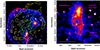 |
Fig. 1. XMM-Newton exposure-corrected mosaic images of SNR W44 region in hard (4.0–8.0 keV) X-ray bands. Left: FoV of W44 with the SNR radio contours in yellow (radio fits file obtained from SNRC at http://snrcat.physics.umanitoba.ca/SNRrecord.php?id=G034.7m00.4) and the soft (0.5–4.0 keV) X-ray contour of W44 in cyan. The position of PSR B1853+01 is marked by a black cross with a green arrow indicating the direction of the pulsar’s proper motion inferred from the pulsar’s position relative to the SNR center and the axis of symmetry of the PWN. Right: Extended X-ray emission coinciding with the position of PSR B1853+01 inside W44. The position of PSR B1853+01 is marked by a black cross. The inner part of the dashed white lines corresponds to the PWN surrounding PSR B1853+01, while the faint extended emission surrounding the PWN is a possible X-ray “halo”. Note that the edge of the thermal emission from SNR cut the halo into two parts. |
The 267 ms pulsar PSR B1853+01/PSR J1856+0113 (Wolszczan et al. 1991) is located south of W44, well within its radio shell and at the southern edge of the thermal X-ray emission region. PSR B1853+01 slows down at a rate of Ṗ ∼ 208 × 10−15 s s−1, which leads to a characteristic age of τc ∼ 20 kyr and a spin-down luminosity of Ė ∼ 4.3 × 1035 erg s−1. Based on its dispersion measure, the distance to the pulsar is estimated to be ∼3.2 kpc (Wolszczan et al. 1991). Further pulsar-related parameters are listed in Table 1. The similarities in both age and distance for PSR B1853+01 and SNR W44 strongly suggest an association between them.
Parameters of PSR B1853+01.
An extended nebula around PSR B1853+01 was first revealed by Jones et al. (1993) in the radio band. Frail et al. (1996) confirmed the PWN nature of the extended radio emission based on 1) the detection of the pulsar at the apex of a cometary-shaped emission with an extension of about 2.5′ (or about 2.3 pc at d = 3.2 kpc) and 2) a relatively flat spectral index α = −0.12 ± 0.04 (where  ) for the nebula, compared to that for the rest of the SNR (α = −0.33). Harrus et al. (1996) reported the detection of the PWN using ASCA observations (4.0–9.5 keV) where W44 is invisible and a source coincident with the position of the pulsar is evident. High-resolution X-ray observations with Chandra further revealed the cometary tail structure of the PWN trailing the pulsar (Petre et al. 2002).
In this paper we present a detailed X-ray study of PSR B1853+01 and its surrounding nebula based on spatially resolved spectral analysis of this system using archival data from Chandra, XMM-Newton and NuSTAR. The structure of this paper is as follows. In Section 2, we describe the observations used in this work and the data reduction processes. In Section 3, we present our imaging and spectral analysis results, including images obtained from different instruments featuring structures on different length scales, together with improved constraints on their spectral properties. In Section 4, we discuss the obtained results, focusing on the nature of the extended emission around and beyond the PWN of PSR B1853+01, and compare our findings to other similar BSPWNe. Finally, in Section 5 we summarize our results and conclusions.
2. Observations and data reduction
2.1. XMM-Newton
There are in total seven archival observations where PSR B1853+01 and its nebula are found in XMM-Newton’s field of view (FOV). Our study is based on the analysis of four of these archival observations (Obs. ID = 0551060101, 0721630101, 0721630201, and 0721630301), as the three remaining pointings accounted for very short exposures, which could lead to inaccurate results due to flaring background. Details of the used observations are given in Table 2. These observations were taken with the European Photon Imaging Camera (EPIC) onboard XMM-Newton, composed of three cameras: MOS1, MOS2, and pn (Turner et al. 2001; Strüder et al. 2001). EPIC cameras allow for highly sensitive imaging observations over the telescope’s FOV of 30′ in the energy range from 0.15 to 15 keV with moderate spectral (E/ΔE ∼ 20–50) and angular (∼6″ FWHM of the PSF1) resolution. We note that Obs. 0551060101, the only on-axis observations used in this paper, was performed on April 24 2009, after the loss of MOS1 CCD6, whereas for Obs. 0721630101, 0721630201, and 0721630301, these observations were taken with an off-axis angle about 4.5′ on 18, 19, and 23 October 2013, respectively, when neither MOS1 CCD6 nor MOS1 CCD3 were available.
Observation log of the XMM-Newton, Chandra, and NuSTAR data used for analysis.
The analysis reported in this work has been performed using the XMM-Newton Science Analysis System2 (SAS) version 20.0.0, on an Ubuntu 20.04 platform. We also made use of the XMM-Newton Extended Source Analysis Software (XMM-ESAS) and related analysis procedures3, since we are mostly interested in the extended emission around and beyond the PWN of PSR B1853+01.
To reduce the data retrieved from the XMM-Newton Science Archive, emchain and epchain were first applied to both MOS and pn observations to filter events based on good time intervals, malfunctioning pixels, and out-of-time events. The task espfilt was then applied to filter out cosmic soft proton events (for pn we set rangescale=15.0).
For the imaging analysis, we generated the spectra for the entire region, the redistribution matrix files, and the ancillary response files, using mos-spectra and pn-spectra, for MOS and pn detectors, respectively. We estimated the non-X-ray background (NXB) with mos-back and pn-back. The merge_comp_xmm tool was then used to merge the individual components (counts, exposure, particle background) from the four observation data sets. We then obtained background-subtracted, exposure-corrected, and adaptively smoothed images using adapt_merge. For the spectral analysis, we first used especget to extract spectra for individual pointings. Then, epicspeccombine and grppha were used to combine and group the spectra.
2.2. Chandra
Three observations (ObsID. 1958, 5548, 6312) containing PSR B1853+01 and its nebula were found in Chandra’s archive (see Table 2 for details). These observations were performed with the Advanced CCD Imaging Spectrometer (ACIS) (Garmire et al. 2003), in timed exposure (TE) mode, without using any gratings. ACIS features two arrays of CCDs: ACIS-I, optimized for imaging wide fields, and ACIS-S, the one used in this study, which provides high-resolution on-axis imaging capabilities. ACIS-S consists of six chips (S0−S5; the S1 and S3 chips being back illuminated) and has a FOV of 8.4′×51.1′. ACIS-S operates in the energy range 0.2–10 keV, with an energy resolution E/ΔE ∼ 5 − 40. The angular resolution is only limited by the size of the CCD pixels (0.492″). For on-axis imaging, ∼85% of the encircled energy lies within ∼1.8″ of the central pixel4. Among the three observations used in this work, ObsID. 5548 and 6312 are on-axis observations on PSR B1853+01 and its PWN (aim point on S3), whereas ObsID.1958 aimed at the center of the SNR W44, with a telescope roll angle of ∼285° and PSR B1853+01 fell on the S2 chip with an off-axis angle of about 7′.
We reduced the data using the Chandra Interactive Analysis of Observations, CIAO (version 4.14.0)5, together with the calibration database CALDB version 4.9.66. All three observations were reprocessed using chandra_repro, while for ObsID. 5548 and 6312, “check_vf_pha = yes” was set to reduce the ACIS particle background in very faint (VFAINT) mode observations.
Broad-band (0.5–7.0 keV) flux images accounting for the three Chandra observations were produced using fluximage (with the parameter psfecf=0.9 to detect faint sources). These flux images were used later by vtpdetect to detect and exclude sources. We checked for flares by filtering the background light curve (0.5–7 keV, time-bin width of 259.28 s) for deviations larger than 3σ using CIAO’s deflare tool. The output good time intervals were then used to filter the events file. No significant flares were detected in ObsID. 5548 and ObsID. 6312, accounting for unchanged exposure time of 52.31 ks and 39.58 ks, respectively, whereas for ObsID. 1958, there are only 44.79 ks left after background flares were removed. The total exposure for the three observations amounts to ∼136.86 ks.
We also applied astrometric corrections to the data sets using the longest observation, ObsID. 5548, as the reference. We used fluximage (with parameter psfecf=0.393, to have bright, point-like sources detected) to generate broad-band flux images that were later used by wavdetect to obtain source lists of each observation. After cross-matching the resulting lists obtained for ObsID. 1958 and ObsID. 5548 and then between ObsID. 5548 and ObsID. 6312 with wcs_match, we corrected for the aspect solution of ObsID. 1958 and ObsID. 6312 with wcs_update. After this astrometry correction, merg_obs was then used to merge observations. For spectral analysis, specextract was used to extract spectra from individual observations while grppha was subsequently used for grouping the spectra.
2.3. NuSTAR
The Nuclear Spectroscopic Telescope Array (NuSTAR) observed the southern part of W44, containing PSR B1853+01 and its PWN, on Sepetember 2, 2018 (ObsID. 40401005002) for a total of ∼105 ks.
NuSTAR is a focusing high-energy (3–79 keV) X-ray observatory (Harrison et al. 2013) featuring two co-aligned telescopes designed with conical Wolter-I type optics modules (OMA and OMB) that are paired with two solid-state detector focal-plane modules (FPMA and FPMB). With a focal length of 10.14 m, NuSTAR’s focal plane covers a FOV of ∼12′. NuSTAR can reach sub-arcminute spatial resolution, with a PSF with an FWHM of 18″ and a half-power diameter of 58″, which is relatively constant across the FOV. It also has good spectral resolution, with an energy resolution (FWHM) of ∼400 eV at 10 keV.
NuSTAR data used in this work were reduced using the NuSTARDAS package (version 2.1.1), along with NuSTAR FPM caldb (version 20220105). nupipeline was used to reprocess the data to produce cleaned and calibrated event list files. For the imaging analysis, we first selected photon events in different energy bands using CIAO tool dmcopy. These energy bands were selected to ensure sufficient photon statistics in each image, as well as to minimize the effects of averaging the energy-dependent vignetting effect over the chosen energy range. We also used nuexpomap to produce exposure maps for each energy band, both for FPMA and FPMB. Then summing up NuSTAR raw images in each energy band with these exposure maps, we created the final mosaic images using XIMAGE (HEAsoft 6.29). For spectral analysis, we used nuproducts to extract spectra for different regions in the FOV, with the parameter “rungrppha=yes” to generate grouped spectra.
3. Analysis and results
The analysis of the data obtained with XMM-Newton, Chandra, and NuSTAR as described above provides complementary information on PSR B1853+01 and its nebula accounting for the unique strengths of each instrument. Chandra offers an excellent angular resolution, which allowed us to separate the pulsar emission from that coming from the surrounding PWN and to resolve out structures on small scales. XMM-Newton, featuring a unique sensitivity and a relatively large FOV, can be used to access the large-scale structures of low surface brightness around the PWN. Finally, the analysis of the NuSTAR data is used to constrain the emission at hard X-rays, revealing for the first time the PWN in X-rays at energies above 10 keV. Below, we detail the obtained imaging and spectral analysis results.
3.1. Imaging
The PWN associated with PSR B1853+01 is hard to resolve at soft X-ray energies. However, it can be discerned from the surrounding SNR above 2.0 keV and becomes the dominant feature in the southern part of W44 above 4 keV (see Fig. 1). We therefore limited our analysis of the PWN to relatively high energies in order to remove the contamination from the SNR thermal emission (a strategy pioneered by Harrus et al. (1996) and also adopted by Petre et al. (2002)).
Figure 2 presents X-ray images of PWN B1853+01–the region immediately surrounding PSR B1853+01–obtained with Chandra (4–8 keV), XMM-Newton (4–8 keV), and NuSTAR (4–10 keV). Here, we selected similar energy bands and also made efforts to closely match the pixel size and smoothing strategy across the three instruments, to ensure a consistent characterization of this region. In particular, the XMM-Newton counts map was produced using only MOS data from the on-axis observation Obs. 0551060101, as this selection provided the best resolution XMM-Newton could achieve. The Chandra and XMM-Newton images reveal complex diffuse X-ray structures surrounding the pulsar: an extended emission around the position of the pulsar stretching in the NW-SE direction, a trail of emission extending further to the northwest, and in addition, an extended emission detected to the south of the pulsar. On larger scales beyond the zoomed-in view of the field shown in Fig. 2, a faint, halo-like, diffuse emission encompassing the PWN is clearly resolved by XMM-Newton as shown in Fig. 1.
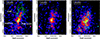 |
Fig. 2. Images of PSR B1853+01 (position marked by a black cross) and its surrounding emission. Left: Exposure-corrected merged Chandra ACIS image in the 4–8 keV energy band, created by combining all three archived observations. The green contours show the radio emission from the PWN (radio FITS file obtained from SNRC at http://snrcat.physics.umanitoba.ca/SNRrecord.php?id=G034.7m00.4). The image is binned by a factor five (pixel size = 2.46″). The dashed yellow line shows the approximate symmetry axis of the PWN tail, which can be divided into two subregions: a compact nebula (CN) surrounding the pulsar and a trail emission further out. The dashed magenta line indicates the N-S direction which roughly coincides with the direction of the outflow just leaving the PWN bow shock. The position of a nearby source 2CXO J185613.6+011207 is marked by a black X. Middle: Merged (MOS1+MOS2) mosaic on-axis (Obs. 0551060101) XMM-Newton counts image in the 4–8 keV energy band (pixel size = 2.5″). Right: Merged (FPMA+FPMB) mosaic NuSTAR image in the 4–10 keV band (pixel size = 2.46″), together with the contour map (in cyan) extracted from the Chandra image shown in the left panel. All images were smoothed with a Gaussian kernel of r = 3 pixels and σ = 1.5 pixels. |
Full-frame NuSTAR images merging two FPMs were created in the energy bands: 4–10 keV, 10–20 keV, and 20–79 keV. Due to the absence of significant source detection in the 20–79 keV range, we only show the 4–10 keV and 10–20 keV NuSTAR images in Fig. 3. We note that this is the first detection of this PWN above 10 keV, and reaching ∼20 keV. Moreover, in the 4–10 keV NuSTAR image, a faint extended feature is found at the same location as the large-scale structure revealed in the XMM-Newton images south of the PWN.
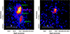 |
Fig. 3. Merged (FPMA+FPMB) NuSTAR images obtained in increasing energy bands. Images are smoothed with a Gaussian kernel of r = 8 pixels and σ = 4 pixels. The position of PSR B1853+01 is marked by a black cross, while the position of a nearby source, 2CXO J185613.6+011207, is marked by a black X. Left: 4.0–10.0 keV image shows an extended emission that coincides with the position of PSR B1853+01, exhibiting a spindle-like shape tapering at both ends and a faint extended emission in the south. Regions used for spatially resolved spectral analysis are shown here. Pulsar spectra were extracted using the magenta circles of two different radii 18″/29″. Region A is similar to the outflow region, Region C is similar to the trail region and Region D is similar to part of the southern halo where one of the large antenna feature lies. The background region is shown by dashed green circle. Right: 10.0–20.0 keV image. The PSR+PWN system is detected up to energies of ∼20 keV. |
3.1.1. The pulsar B1853+01
Between the first off-axis (obs. 1958) and the later two on-axis (obs. 5548,6312) Chandra observations, about four years and seven months, we detect no significant shift of pulsar position. The two on-axis Chandra observations (Obs. 5548 and 6312) were used to further study the compact source. An unbinned and unsmoothed count image in the Chandra hard energy band (2.0–7.0 keV) made by combining the two observations is shown in Fig. 4. In this energy range, the emission from the pulsar dominates that from the surrounding PWN and also that from the SNR thermal emission. We performed source detection on the combined counts image using wavdetect with both PSF and exposure maps supplied as inputs and pinpointed the pulsar position at RA(J2000) = 18h56m10 68, Dec(J2000) = +01°13′22
 87. In Table 3, we summarize the positions of PSR B1853+01 obtained from previous timing observations in the radio band, from previous X-ray measurements as well as from our own work. The errors given in the Chandra measurements include both statistical and systematic uncertainties. A comparison of Chandra and radio positions implies a transverse velocity significantly higher than that estimated by Frail et al. (1996) based on the position of the pulsar within the SNR. However, this discrepancy may arise from underestimated uncertainties in radio position reported by Jacoby et al. (1999), as PSR B1853+01 exhibits substantial intrinsic timing noise. We noticed that in the XMM-Newton MOS image of the region surrounding PSR B1853+01 created from Obs. 0551060101, the centroid of the brightest pixel is located ∼4″ north to the position determined as mentioned above from Chandra on-axis observation data. We thus further examined the images produced from Obs. 721630101, 721630201, and 721630301 and found that the centroids of the brightest pixels in these images coincide with the Chandra pulsar position. We conclude that a relatively small position offset is present in Obs. 0551060101. On the other hand, the centroid of the brightest pixels in the 4.0–20.0 keV NuSTAR mosaic image is ∼6″ away from the derived Chandra pulsar position, yet it is within NuSTAR’s absolute astrometric uncertainty of 8″ for the brightest targets (90% confidence; Harrison et al. 2013).
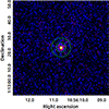 |
Fig. 4. Chandra 2–7 keV on-axis unbinned and unsmoothed counts image. Circle and annulus are centered at the pulsar position detected by Chandra. The magenta circle has a radius of 1.8″ and was used for the extraction of the pulsar spectra; the dashed green annulus, with inner and outer radius of 3″ and 6″, was used as the background region. |
Position of PSR B1853+01.
3.1.2. The PWN tail
The merged Chandra image (Fig. 2, left panel) reveals a cometary-shaped “tail” emission, which is elongated in the southeast-northwest direction, approximately along a line with a position angle of ∼20° (north through west). This tail feature, extending up to ∼1.5′ (or 1.4 pc at d = 3.2 kpc) on the northern side of the pulsar, is located inside of the thermal emission boundary of the SNR and is about half the extent observed at radio wavelengths. A gap halfway along the tail is clearly visible in the Chandra image (also in XMM-Newton and NuSTAR images), dividing the tail morphologically into two subregions: a “near” half identified as the compact nebula (CN) in the pulsar’s close vicinity, and a “far” half referred to as the “trail” region. The CN is the second brightest feature in the field, about ten times fainter than the pulsar, whereas the extended trail emission is relatively dimmer with an average surface brightness approximately half that of the CN. A hint of a small extended feature, at an angle to the pulsar’s proper motion direction (protruding to the northeast just behind the pulsar), of a similar brightness to the trail region, is also apparent in the Chandra image and renders the tail emission less symmetric.
3.1.3. The outflow
We identified an extended region of emission, the “outflow”, preceding the pulsar with a surface brightness similar to that of the trail region. This emission region, which lies mostly outside of the thermal emission boundary of the SNR, extends as far as ∼1′ (or ∼1.0 pc at d = 3.2 kpc) to the south of the pulsar and covers approximately 1000 arcsec2 in the sky. A total of 3202 source counts were retrieved from this outflow region, whereas about 2522 background counts are estimated, yielding 680 excess counts, implying an ∼9σ statistical significance assuming a Gaussian approximation. Best resolved by Chandra, this outflow feature exhibits a morphology resembling a pair of “antennae.” The 4–8 keV Chandra image in Figure 2 shows an extended emission that protrudes from the southern vicinity of the pulsar, subsequently breaking into two filamentary branches while a gap in the emission is discernible halfway before the branching. One of the southern branches continues in the southern direction, whereas the other extends toward the southwest. XMM-Newton, on the other hand, can barely resolve this extended feature from the CN+PSR emission, yet it detects the gap between the protruding stem and the southern branching part. These findings are in good agreement with the Chandra image presented in Petre et al. (2002), where hints of this extended region of emission appeared as part of a fainter subregion used for spectral analysis there.
3.1.4. An X-ray halo
A relatively fainter yet more extended emission, encompassing the central PWN is discernible in XMM-Newton image in Fig. 1 and Fig. 6. This extended emission, which we tentatively identify as an X-ray “halo,” displays an average surface brightness dimmer than that of the PWN by a factor of ∼3. The halo region can be further divided into the northern and southern parts based on the boundary of the thermal SNR X-ray emission. The northern part of the X-ray halo follows the overall shape of the PWN tail, extending only ∼0.5 arcmin outward from the PWN. In contrast, the southern part has a diffuse, large-scale antennae-like morphology, reaching distances of about 6′/3′ (or 6.0/3.0 pc at d = 3.2 kpc). This prominent large-scale southern halo feature appears to extend from the central PWN, in the very same direction as the smaller and brighter inner feature – the outflow – observed at closer distances south to the pulsar.
Our results from NuSTAR confirm the existence of the large-scale structure (left panel in Fig. 3) with a morphology closely resemble that obtained with XMM-Newton, despite possible distortion caused by chip gaps in the NuSTAR data. We also searched for this large-scale structure in Chandra images. This was prevented, however, by the orientation of the ACIS array, as the two on-axis observations failed to cover this area. Only in Obs.ID 1958 is this region covered, but most of the feature extension falls on the edge of the S2 chip and the back-illuminated S1 chip.
3.2. Spectral results
In our spectral analysis, spectra were extracted from the following regions: (1) the pulsar region; (2) the PWN tail region (CN+trail; excluding the pulsar itself); (3) the outflow region ahead of the pulsar; and (4) the faint halo region encompassing the three aforementioned regions. We also defined several background regions to be used in the spectral fits. The XSPEC (Arnaud 1996) software (version 12.9.0) was used for the spectral analysis. The Tuebingen-Boulder ISM absorption model tbabs with abundances taken from Wilms et al. (2000) were used to calculate the X-ray absorption in the ISM. Uncertainties are given at a 90% confidence level unless specified otherwise.
3.2.1. The pulsar B1853+01
The thermal contamination from the SNR in the soft X-ray band (below ∼4 keV) significantly impacts the spectral analysis of the whole PWN. The pulsar itself might be in this regard the less affected region given its point-like nature. The spectral analysis on PSR B1853+01 was therefore used to determine the column density, NH, toward the system.
For the analysis of Chandra data, a circular region with a 1.8″ radius centered at RA(2000) = 18h56m10.69s, Dec(2000) = 01° 13′22.9″ was defined as the extraction region for PSR B1853+01. To remove the contamination from the PWN, the background region was chosen to be a 3″ − 6″ annulus centered on PSR B1853+01 (see Fig. 4). The spectra were extracted from the three Chandra observations and were combined and grouped to have a minimum of 20 cts/bin. We then fit the pulsar spectra from 0.5 to 8 keV using different models. By applying an absorbed power-law emission model, “tbabs × PL”, the best fit yields a column density of  cm−2, a photon index of
  , a normalization of
  photons/keV/cm2/s, and an observed flux in the 0.5–8.0 keV band of 4.12 × 10⁻¹⁴ erg cm−2 s−1 (χred2 = 1.01 with 16 degrees of freedom, null hypothesis probability of 0.44). We also note that middle-aged pulsars often have a thermal component in the pulsar spectrum. However, fitting the pulsar spectra with an absorbed black-body model alone (“tbabs × BB”) gives an unrealistically low column density with a large associated error. Parameters could not be well constrained when fitting the pulsar spectra with an absorbed black-body plus a power-law emission model, tbabs × (BB + PL), either. We also tried to extract the pulsar spectra with other different background regions drawn from nearby fields. Fit results were insensitive to the specific choice of background region. Finally, as a further check, we also considered deriving the NH value from the CN region, the spectrum of which is expected to be a pure power law only modified by the ISM absorption. The results of the spectral fit are, however, highly sensitive to the choice of the background regions. Using the background region “bkg1” defined as in Figure 5, the best-fit NH value from the CN region is
  cm−2 (χred2 = 1.11 with 145 degrees of freedom, null hypothesis probability of 0.18).
Our best-fit pulsar photon index  differs noticeably from the significantly harder spectrum, Γ = 1.28 ± 0.48, reported in Petre et al. (2002). We noticed that these authors considered a much higher column density NH ≈ 5 × 1022 cm−2, possibly referencing an incorrect value from Rho et al. (1994), as the two sub-figures describing the temperature and column density distributions of W44 region by region in Fig. 10 of Rho et al. (1994) are wrongly labeled (according to the values in their Table 4). The value of NH reported here is, however, consistent with what was obtained by Harrus et al. (2006) where the pulsar spectrum was extracted from a radius of 20″ centered at RA(2000) = 18h56m11s, Dec(2000) = 01° 13′24″, using XMM-Newton Obs. 0083270301 and 0083270401. In Harrus et al. (2006), the spectrum was best described with an absorbed power-law model with
  using NH = 0.6 ± 0.2 × 1022 cm−2, which is a column density value slightly lower than what they obtained for the entire remnant. Harrus et al. (1996), on the other hand, presented ASCA analysis of the X-ray synchrotron nebula associated with PSR B1853+01 where data were extracted from a circular region of radius 5′(3′) centered on the radio pulsar position, obtaining a photon index of
  and a column density of NH = (1.82 ± 0.05)×1022 cm−2. The moderate discrepancy with our results might not be surprising as the extraction regions applied are much larger, in contrast to the Chandra capabilities in spatially resolving the different structures.
For XMM-Newton data, given the different PSFs of the detectors, we defined pulsar extraction regions of different sizes. For Obs.551060101, we used circular source regions of 7″/9″ (MOS/pn) and concentric annuli background regions of 8″–11″ (MOS) and 10″–13″ (pn). For other off-axis observations, source radii were 9″/11″ (MOS/pn), with background annuli of 10″–13″ (MOS) and 12″–15″ (pn). Extracted spectra were combined and grouped to ≥30 cts/bin. Fitting the spectrum in 0.5–10 keV gives an absorbed power law with  and
and  (see Table 4), consistent, within errors, with Chandra results. In the remainder of the spectral analysis, NH = 0.65 × 1022 cm−2 will be used. For NuSTAR data, pulsar spectra extracted from an 18″/29″ circular region fixed at the centroid of the brightest pixels were grouped to have at ≥200 cts/bin. When applying an absorbed power-law model with NH fixed, we obtained a best fit in 3–10 keV with
  , χred2(d.o.f.) of 1.20 (15) (see Table 4)/
  , χred2(d.o.f.) of 0.75 (36).
Best-fitting values for PSR B1853+01.
3.2.2. Spatially resolved spectral analysis
Spatially resolved spectra of the extended emissions surrounding the pulsar were extracted from different regions in Chandra, XMM-Newton, and NuSTAR data sets.
For the three archived Chandra observations, weighted spectra were extracted from the PWN tail region (CN+trail) and the outflow region, as shown in Fig. 5. The imaging analysis results in Sect. 3.1 reveals that the PWN tail is located inside the boundary of the SNR thermal X-ray emission while most of the outflow region lies outside and the whole PWN is surrounded by a relatively fainter halo-like structure (see Sect. 3.1.4). For the PWN tail region, we chose a background region (denoted as “bkg1” in Fig. 5) similar to the part of the halo structure inside the boundary of the SNR thermal X-ray emission. For the outflow feature a background region was taken from the halo structure outside of the boundary of the SNR thermal X-ray emission but still enclosing the outflow region (denoted as “bkg2” in Fig. 5). The weighted spectra extracted from the two regions were combined and grouped, respectively, to have at least 20 cts/bin and fit with an absorbed power-law model, “tbabs × PL”. In Table 5, we present the best-fit results from fitting the spectra extracted from the two regions. The tail spectra were fit from 3.0 to 8.0 keV (to minimize the effect of the residual thermal emission) with the column density fixed at 0.65 × 1022 cm−2, yielding a photon index of  , χred2 = 0.98 (d.o.f. = 53) for this tail region. We tried to extract and fit the spectra from the two subregions (CN and trail) of the tail structure, but the low statistics restricted us from obtaining meaningful results after cutting out the thermal radiation below 3 keV. The spectra extracted from the outflow region were fit on the other hand from 0.5 to 8.0 keV, and the best-fit results give a rather hard photon index of
  .
.
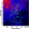 |
Fig. 5. Merged Chandra broad band (0.5–7.0 keV) flux image with extraction regions used for spectral extraction overlaid. The image is unbinned yet smoothed with a Gaussian function with radius r = 3 pixel and sigma σ = 1.5 image pixels. Weighted spectra have been extracted from tail (solid cyan) region with pulsar (r = 3″) excluded, using bkg1 region (dashed green) as background region, and from outflow region (solid yellow) using bkg2 region (dashed green) as background region. |
Best-fit results from spatially resolved spectra.
For XMM-Newton observations, we only used pn data from Obs. 721630101, 0721630201, and 0721630301. Despite the relative worse spatial resolution of the pn camera, these exposures were chosen as the entire PWN + halo system was captured on one single pn chip. In contrast, other EPIC exposures are compromised and not used for either significant portion of the emission is not available (due to the loss of MOS1 CCD3, which affected Obs ID.721630101, 0721630201 and 0721630301), or the PWN falls in close proximity to chip gaps or bad pixels. We extracted spectra from the PWN tail region, the outflow region and also the halo region as shown in Fig. 6. For the PWN tail and outflow region, background regions are selected in nearby halo regions as shown in the left panel of Fig. 6. Extracted spectra were grouped and combined to have at least 30 cts/bin and were fit using an absorbed power-law model, tbabs × PL, with NH fixed to 0.65 × 1022 cm−2. For the PWN tail, the high sensitivity of XMM-Newton allowed us to split it into two subregions: the CN region and the trail region. For both subregions, we fit the data in the energy range from 3.0 to 10 keV as the low energy part is heavily affected by background subtraction. For the outflow region, since it is outside of the SNR thermal X-ray emission, its spectrum is less affected in the low energy part, and hence we fit it from 0.5 to 10.0 keV. A summary of the spectral fitting results is given in Table 5. We also tried to extract spectra from the halo region and its two subregions as shown in the right panel of Fig. 6. Spectra from the two subregions were combined and grouped to have at least 200 cts/bin due to the low surface brightness of this halo feature. We limited the fit from 3.0 keV to 7.5 keV to the halo spectra as they are rather noisy below 3 keV, and copper line emission due to the detector itself is present in the high-energy end outside of the fit range.
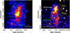 |
Fig. 6. Left: 4′ × 4′ XMM-Newtonpn image in 4.0–8.0 keV band (merged from Obs. 0721630101, 0721630201, and 0721630301). The extraction regions for the tail region (solid cyan; crossed green circle region representing PSR B1853+01 was excluded from the CN/tail spectral analysis) and the outflow region (solid magenta) are shown. The tail region can be further split into two subregions: CN and trail (separated by the line). A background region inside the thermal X-ray emission area BKG1 (dashed green) was chosen for the tail regions while the outside BKG2 (dashed green) was chosen for the outflow. Right: 12′ × 12′ XMM-Newtonpn image in 4.0–8.0 keV band (merged from Obs. 0721630101, 0721630201, and 0721630301). The extraction regions for the halo region are shown. The halo region is divided into two subregions: the northern halo (solid white) and the southern halo (solid green). Background regions (dashed yellow lines) for these two regions of interest are BKG3 and BKG4, respectively. The point source (shown by the crossed green circle) that appears in the southern halo region was excluded from the halo spectral analysis. |
For NuSTAR observations, spectra were extracted from extended regions A, C, and D as shown in Fig. 3. Region A is similar to the outflow region, region C is similar to the trail region, and region D is similar to the part of the southern halo where one of the large-scale antenna feature lies. We fit the NuSTAR spectra in the 3 to 20 keV band with an absorbed power-law model, tbabs × PL, fixing the column density value at NH = 0.65×1022cm−2. The photon index parameter is linked for the two detector modules, whereas normalization parameters were allowed to vary to take into account the small relative calibration uncertainties between the two modules. Our best-fit results are presented in Table. 5.
4. Discussion
4.1. BSPWN B1853+01 inside of SNR W44
In general, the evolution of the PWN is coupled to that of its associated SNR until either the pulsar overtakes the blast wave (at crossing time tcr) or the SNR dissipates. Born with a given kick velocity, a pulsar powers a PWN that is initially expanding supersonically into the freely expanding SNR ejecta. When the PWN shock interacts with the SN reverse shock, the PWN bubble oscillates back and forth due to the reverberations from the passage of the reverse shock. Later, the reverberation vanishes and the PWN expands subsonically. Eventually, when the pulsar is positioned at ∼2/3 of the radius of the supernova remnant blast wave, a bow shock is formed around the head of the PWN due to the mildly supersonic motion of the pulsar (van der Swaluw et al. 2004), which might be the case here for BSPWN B1853+01 inside the SNR W44. Following the formation of the bow shock, the Mach number will slowly increase following the decrease of the sound speed as the PWN approaches the SNR Shell (see, e.g., the location of the BSPWN in SNR CTB80, close to the SNR shell; Safi-Harb et al. 1995; Migliazzo et al. 2002; Li et al. 2005). Once the pulsar breaks through the shell, its dynamics are no longer affected by the parent SNR and it will continue being accompanied with a BSPWN for its supersonic motion in the ISM. BSPWNe are thus usually formed during the last stages of PWN/SNR evolution.
PSR B1853+01 is estimated to be moving to the south with a transverse velocity of ≲370 km s−1 (±25 km s−1) for the pulsar is displaced about 8′.6 ± 0′.5 away from the SNR center and the age for the SNR/PSR system is τc ∼ 20 kyrs (Frail et al. 1996). The tail that we observed in X-rays extending about ∼1.5′ to the north confirms that the pulsar is indeed moving supersonically to the south. The pulsar wind is confined by the ram pressure,  (RTS is the stand-off distance, c is the speed of light, ρ0 is the density of the ambient medium, and vPSR is the pulsar’s velocity relative to the medium). Compared to other BSPWNe moving in the ISM, PWN B1853+01 has a rather compact size, with the tail extending only for about 1.4 pc. This is probably due to the existence of the high thermal pressure of the hot X-ray emitting gas in W44, Pplasma ∼ 1.1 × 10⁻⁹ erg cm−3, several orders of magnitude higher than the pressure of the ISM (Harrus et al. 1997). The X-ray tail emission is likely due to synchrotron radiation from the shocked pulsar wind. The size of this X-ray tail is about half the extent observed in radio which is probably due to a shorter synchrotron loss timescale for X-ray emitting electrons. The gap detected in the tail region in our X-ray imaging analysis, corresponding approximately to the “kink” feature observed in radio observations (Frail et al. 1996), could possibly be produced due to the passage of the reverse shock. The photon index of the tail region (
 ) is consistent with those of a typical PWN, which have nominal ranges of Γ ∼ 1.1 − 2.4 (Gaensler et al. 2006).
The Chandra imaging results in Sect. 3.1.2 shows that the angular separation from the pulsar position to the edge of the extended CN in the direction of the pulsar motion is about 8″. However the true location of the termination shock is expected to be much closer to the pulsar than the edge of the CN. In the case of the Crab Nebula, for example, it is located at ∼10% of the outer radius of the luminous nebula. Assuming that the pulsar is located 3.2 kpc away and is moving in the plane of the sky and taking 10% of this as the standoff separation angular distance, it yields an estimated standoff radius, RTS, of approximately 0.01 pc. For a particle density ne = 0.25 cm−3 near PSR B1853+01 inside W44 (Jones et al. 1993), assuming cosmic abundances, this corresponds to a mass density of ∼1.2 × 10⁻²⁴ g/cm3. The velocity of the pulsar is thus  km/s. Our estimate is consistent with that inferred from its relative position to the center of the SNR and its age. However, in both estimations, only the transverse component is accounted for. A precise measurement of the full 3D velocity would require observations with current radio interferometer facilities such as VLA and MeerKAT.
4.2. Outflow in BSPWN B1853+01
The presence of an outflow preceding PSR B1853+01 clearly visible in the hard X-ray energy band (above 2 keV) taking a morphology of an antennae-like structure is puzzling. The verification of the nature of this emission as non-thermal ( ) and its association with the pulsar could have strong implications for our understanding of the system.
Jet-like structures have been detected in PWNe associated with supersonically moving pulsars, e.g. in Geminga (Posselt et al. 2017), PWN B1929+10 (Hui & Becker 2008) and PWN J1153+6055 (Bordas et al. 2021). These structures could be interpreted in the context of genuine pulsar jets, which are found to be bent by the ram pressure of the surrounding medium, forming the observed arc-shaped structures. The cometary tail trailing the pulsar in these systems corresponds to a motion-distorted torus, or as part of the limb-brightened shocked pulsar wind. Recent numerical simulations of fast-moving PWNe (Barkov et al. 2019), where the influence of geometric factors on the magnetic structure in the shocked pulsar wind are consistently addressed, provide further support to this scenario. On the other hand, misaligned X-ray outflows detected in a number of BSPWNe are difficult to interpret as pulsar jets or shocked pulsar wind structures, such as the filaments detected in the Guitar Nebula (Hui & Becker 2007; Wang 2021), the Lighthouse Nebula (Pavan et al. 2014, 2016), PWN J2030+4415 (de Vries & Romani 2022), the northern outflow in PWN J1509-5850 (Klingler et al. 2016a) or the “whisker” features in the Mushroom Nebula (PWN B0355+54) (Klingler et al. 2016b). These non-bent misaligned features may be instead produced by high-energy particles escaping the PWN bow shock region through reconnected magnetic field lines, emitting synchrotron emission that traces the ISM magnetic field, a scenario originally proposed in Bandiera (2008).
Highly energetic particles might be able to escape the PWN when their gyro-radius is comparable or exceeds the stand-off distance of the bow shock. For electrons emitting synchrotron radiation at a few keV in a (possibly amplified) magnetic field B∼ few ×10 μG (see e.g. the derived values for the Guitar and the Lighthouse Nebula in Olmi et al. (2024)), Lorentz factors of γ ∼ 108 are required. These electrons will therefore be able to escape the parent PWN if the bow shock is shorter than their gyro-radii, which at these energies γ and B values is rg∼ few × 1015 cm. Although this particle leakage mechanism is supported by recent 3D MHD simulations (Barkov et al. 2019; Olmi & Bucciantini 2019), our Chandra data could not constrain the bow shock radius further than ∼RTS ≳ 0.01 pc, or about ∼3 × 1016 cm, as derived above.
PSR B1853+01 is moving at the edge of the thermal X-ray emission region inside the SNR W44, where the pulsar possibly has experienced or is experiencing a relatively abrupt change of environment conditions. The sudden decrease in density of the surrounding ejecta might not be able to effectively confine particles in the shocked wind anymore. Another possibility is that the pulsar wind shock has already interacted with the reverse shock, leading to an enhancement of high-energy particles escaping the bow shock region and streaming farther out. In this scenario, the orientation of the outflow feature observed in PWN B1853+01 might indicate the local magnetic field structure. The magnetic field geometry inside W44 inferred from both CO and HCO+ seems indeed oriented along the north-east direction and showing almost almost insignificant intensity variations (Liu et al. 2022).
The spectral analysis in Sect. 3.2.2 reveals that the outflow feature in PWN B1853+01 has a relatively harder spectrum compared to that of the pulsar or the PWN tail ( /
/  from Chandra). In fact, misaligned outflows discovered in other BSPWNe sources usually display relatively hard spectra (
 , ΓJ1101 = 1.7 ± 0.1, ΓJ2030 = 1.18 ± 0.20, ΓJ1509 = 1.50 ± 0.20, and
  in the 0.5–8 keV band). This could be a fingerprint of the energy-selection process leading to the formation of such structures in a particle-escape scenario.
It is also worth noting that in the Galactic Center region, a number of X-ray filaments have been detected by Chandra and XMM-Newton (Johnson et al. 2009; Wang et al. 2002). Numerous narrow radio filaments have been reported by MeerKAT (Heywood et al. 2022) (see also Khabibullin et al. (2024), which reported the discovery of a radio filament located ahead of PSR J0538+2817). These filaments could be streams of high-energy particles escaping yet unidentified PWNe, with the radio ones representing the low-frequency analogues of those seen in X-rays (Barkov & Lyutikov 2019; Bordas et al. 2021).
4.3. Halos in BSPWNe
The faint, halo-like extended X-ray emission encompassing the central core PWN B1853+01 is particularly notable as it closely follows the morphology of the central PWN in almost all directions. Specifically, the southern part of the halo takes precisely the same shape as the outflow feature observed just ahead of the pulsar. The detection of this large X-ray halo is, in fact, consistent with the results obtained from ASCA observations (see, e.g., Fig. 1 in Harrus et al. (1996)), in which an elongation of the PWN toward the south in both the 4.0–9.5 keV GIS and SIS maps is apparent. These authors then noted that the position of the hard X-ray source they detected at the position of the pulsar is marginally inconsistent with the peak position of the diffuse radio nebula to the north. The 4–8 keV MOS+pn image of SNR W44 in Okon et al. (2020) also strongly suggests the existence of a large-scale structure near the pulsar/PWN position. However, the PWN-related hard X-ray emission was not discussed there.
The extended X-ray emission associated with PWN B1853+01, on the other hand, exhibits striking similarities with that of the Snail PWN inside of SNR G327.1-1.1, the archetype of a PWN/SNR system in its late-time evolution stage. In the core nebula of the Snail PWN, a compact source is located at the apex of a tail of X-ray emission that extends in the southeast direction, while two prong-like structures protrude northwest from the head of the bow shock. The whole core nebula is embedded in a faint diffuse emission where the two prong-like structures seem to be extending into large arcs (Temim et al. 2009, 2015). Note that extended TeV emission from this region has been reported (HESS J1554-550, H.E.S.S. Collaboration 2018). The physical size of this diffuse TeV emission is approximately equivalent to that of the TeV halo discovered around the Geminga PWN.
A scenario in which energetic electrons having escaped the PWN diffuse into the ambient medium could explain the faint halo emission observed in X-rays significantly larger than the size of the PWNe and, in the case of Snail PWN, the emission in the TeV band. In the 1LHAASO catalog as well as in the 2HWC catalog, a large fraction of sources are claimed to be spatially coincident with pulsars/PWNe (Cao et al. 2024; Abeysekara et al. 2017b), suggesting that TeV halo or particle escape from PWNe is a generic feature related to pulsar/PWN emission. The particle escape process could possibly first appear in the late evolution stages of the PSR/SNR system (e.g., in BSPWN B1853+01 and in the Snail PWN) due to the passage of the reverse shock which crashed the quasi-steady PWN (Giacinti et al. 2020). These electrons diffuse into the more distant region where they interact with the ambient photon field and are responsible for the IC radiation observed in the TeV energy band and also possible extended synchrotron radiation in X-rays whereas the ratio of the X-ray and TeV halo intensities, Psyn/PIC = uB/uph would depend on the ratio of the energy density between the magnetic field and the scattering photon field (Aharonian et al. 1997; Linden et al. 2017).
So far, no confident detection of emission at GeV or TeV energies have been reported from PWN B1853+01. The 95% confidence contour for the EGRET source 3EG 1856+0114 coincides with the southeastern sector of the SNR W44 where PWN B1853+01 is located (Thompson et al. 1996). While the reported GeV was interpreted by de Jager & Mastichiadis (1997) in terms of relativistic bremsstrahlung and IC scattering produced by a power-law distribution of relativistic electrons injected by PSR B1853+01, an alternative possibility is that a significant part of the gamma-ray flux observed may also be due to SNR shell-cloud interactions. In this regard, GeV emission has been recently reported from two extended structures located at the two opposite ends of the remnant along its majors axis (Uchiyama et al. 2012; Peron et al. 2020). Interestingly, the southern structure lies close to the position of the PWN, although its spectral properties and vicinity to enhanced gas density regions strongly suggest an SNR-cloud interaction for its origin (Peron et al. 2020). On the other hand, VHE gamma-ray fluxes at the level of 0.1 Crab are expected to be detected around PSR B1853+01 (Aharonian et al. 1997), yet no VHE gamma-ray observation pointed to the immediate vicinity of the PWN has been reported so far. VERITAS has reported upper limits to the VHE flux from the W44 region at a level of ∼1.2 × 10 erg s−1 cm−2 in the 0.5–5.0 TeV range (Archer et al. 2025). MAGIC, on the other hand, recently studied the northwestern region of W44, with no firm detection of any VHE counterpart (Abe et al. 2025). No sources coincident with W44 nor the HE structures, however, were identified neither in the first LHAASO catalog (Cao et al. 2024) nor in the third HAWC catalog (Albert et al. 2020).
5. Conclusions
We have presented a comprehensive analysis of the X-ray emission around PSR B1853+01 using data from Chandra, XMM-Newton, and NuSTAR. An X-ray PWN around PSR B1853+01 of rather complex structures is revealed: a cometary tail stretching along the northwest-southeast direction, of ∼1.5′ (∼1.4 pc) in size, and a small protruding outflow feature, extending toward the south ∼1′ (∼1.0 pc). XMM-Newton observation analysis on the other hand unveiled a faint X-ray halo feature encompassing the central PWN for the first time. The southern part of the halo structure, reaching about 6′ (∼6.0 pc), morphologically resembles the outflow feature, being larger in size and fainter in brightness. At the same position of the southern part of the halo, X-ray emission was also detected with NuSTAR. And for the first time the PWN surrounding PSR B1853+01 was detected above 10 keV up to about 20 keV.
We confirm a non-thermal origin for the outflow feature and for the halo-like X-ray emission, displaying a harder spectrum compared to that of the pulsar or the PWN tail ( /
/  from Chandra,
  from XMM-Newton). We thus propose that both the outflow feature and the halo-like emission region surrounding the whole PWN nebula are produced by energetic particles escaping the PWN bow shock region.
Next-generation X-ray instruments, such as AXIS (Safi-Harb et al. 2023), with excellent angular resolution across a wide FoV and improved flux sensitivity would help to constrain the size of the X-halo structure and, eventually, closely pinpoint the sites of particle acceleration and escape. Finally, radio interferometric observations of BSPWN B1853+01 might help to better constrain the pulsar proper motion velocity and the location of the standoff distance, further constraining the spectrum of the escaping particles.
Acknowledgments
XZ acknowledges funding by l’Agència de Gestió d’Ajuts Universitaris i de Recerca (AGAUR) under the FI-SDUR grant (2021 FISDU 00369). PB and XZ also acknowledges support from Ministerio de Ciencia, Innovación y Universidades (MCIUN) through Proyectos I+D Generación de Conocimiento PID2019-105510GB-C31, PID2022-136828NB-C41 and PID2022-138172NB-C43. SH’s research is primarily supported by the Natural Sciences and Engineering Research Council of Canada (NSERC) through the Discovery Grants and Canada Research Grants Programs. KI acknowledges support under the grant PID2022-136828NB-C44 provided by MCIN/AEI/10.13039/501100011033/FEDER, UE. Authors also thank George Pavlov for his valuable comments that helped to improve the paper.
References
- Abe, S., Abhir, J., Abhishek, A., et al. 2025, A&A, 693, A255 [NASA ADS] [CrossRef] [EDP Sciences] [Google Scholar]
- Abeysekara, A. U., Albert, A., Alfaro, R., et al. 2017a, Science, 358, 911 [NASA ADS] [CrossRef] [Google Scholar]
- Abeysekara, A. U., Albert, A., Alfaro, R., et al. 2017b, ApJ, 843, 40 [Google Scholar]
- Aharonian, F. A. 1995, Nucl. Phys. B Proc. Suppl., 39, 193 [Google Scholar]
- Aharonian, F. A., Atoyan, A. M., & Kifune, T. 1997, MNRAS, 291, 162 [NASA ADS] [CrossRef] [Google Scholar]
- Aharonian, F., An, Q., Axikegu, B. L. X., et al. 2021, Phys. Rev. Lett., 126, 241103 [Google Scholar]
- Albert, A., Alfaro, R., Alvarez, C., et al. 2020, ApJ, 905, 76 [NASA ADS] [CrossRef] [Google Scholar]
- Archer, A., Bangale, P., Bartkoske, J. T., et al. 2025, ApJ, 983, 73 [Google Scholar]
- Arnaud, K. A. 1996, in Astronomical Data Analysis Software and Systems V, eds. G. H. Jacoby, & J. Barnes, ASP Conf. Ser., 101, 17 [NASA ADS] [Google Scholar]
- Bandiera, R. 2008, A&A, 490, L3 [NASA ADS] [CrossRef] [EDP Sciences] [Google Scholar]
- Barkov, M. V., & Lyutikov, M. 2019, MNRAS, 489, L28 [NASA ADS] [CrossRef] [Google Scholar]
- Barkov, M. V., Lyutikov, M., Klingler, N., & Bordas, P. 2019, MNRAS, 485, 2041 [NASA ADS] [CrossRef] [Google Scholar]
- Bogovalov, S. V., & Khangoulian, D. V. 2002, MNRAS, 336, L53 [NASA ADS] [CrossRef] [Google Scholar]
- Bordas, P., Zhang, X., Bosch-Ramon, V., & Paredes, J. M. 2021, A&A, 654, A4 [NASA ADS] [CrossRef] [EDP Sciences] [Google Scholar]
- Cao, Z., Aharonian, F., An, Q., et al. 2024, ApJS, 271, 25 [NASA ADS] [CrossRef] [Google Scholar]
- Caswell, J. L., Murray, J. D., Roger, R. S., Cole, D. J., & Cooke, D. J. 1975, A&A, 45, 239 [NASA ADS] [Google Scholar]
- Clark, D. H., Green, A. J., & Caswell, J. L. 1975, Aust. J. Phys. Astrophys. Suppl., 37, 75 [Google Scholar]
- Claussen, M. J., Frail, D. A., Goss, W. M., & Gaume, R. A. 1997, ApJ, 489, 143 [NASA ADS] [CrossRef] [Google Scholar]
- de Jager, O. C., & Mastichiadis, A. 1997, ApJ, 482, 874 [Google Scholar]
- de Vries, M., & Romani, R. W. 2022, ApJ, 928, 39 [NASA ADS] [CrossRef] [Google Scholar]
- Frail, D. A., Giacani, E. B., Goss, W. M., & Dubner, G. 1996, ApJ, 464, L165 [Google Scholar]
- Gaensler, B. M., Chatterjee, S., Slane, P. O., et al. 2006, ApJ, 648, 1037 [NASA ADS] [CrossRef] [Google Scholar]
- Garmire, G. P., Bautz, M. W., Ford, P. G., Nousek, J. A., & Ricker, G. R. J. 2003, in X-Ray and Gamma-Ray Telescopes and Instruments for Astronomy, eds. J. E. Truemper, & H. D. Tananbaum, SPIE Conf. Ser., 4851, 28 [Google Scholar]
- Giacinti, G., Mitchell, A. M. W., López-Coto, R., et al. 2020, A&A, 636, A113 [NASA ADS] [CrossRef] [EDP Sciences] [Google Scholar]
- Goldreich, P., & Julian, W. H. 1969, ApJ, 157, 869 [Google Scholar]
- H.E.S.S. Collaboration (Abdalla, H., et al.) 2018, A&A, 612, A1 [NASA ADS] [CrossRef] [EDP Sciences] [Google Scholar]
- Harrison, F. A., Craig, W. W., Christensen, F. E., et al. 2013, ApJ, 770, 103 [Google Scholar]
- Harrus, I. M., Hughes, J. P., & Helfand, D. J. 1996, ApJ, 464, L161 [Google Scholar]
- Harrus, I. M., Hughes, J. P., Singh, K. P., Koyama, K., & Asaoka, I. 1997, ApJ, 488, 781 [Google Scholar]
- Harrus, I., Smith, R., Slane, P., & Hughes, J. 2006, in The X-ray Universe 2005, ed. A. Wilson, ESA Spec. Pub., 604, 369 [Google Scholar]
- Heywood, I., Rammala, I., Camilo, F., et al. 2022, ApJ, 925, 165 [NASA ADS] [CrossRef] [Google Scholar]
- Hui, C. Y., & Becker, W. 2007, A&A, 467, 1209 [NASA ADS] [CrossRef] [EDP Sciences] [Google Scholar]
- Hui, C. Y., & Becker, W. 2008, A&A, 486, 485 [NASA ADS] [CrossRef] [EDP Sciences] [Google Scholar]
- Jacoby, B. A., & Wolszczan, A. 1999, in Pulsar Timing, General Relativity and the Internal Structure of Neutron Stars, eds. Z. Arzoumanian, F. Van der Hooft, & E. P. J. van den Heuvel, 157 [Google Scholar]
- Johnson, S. P., Dong, H., & Wang, Q. D. 2009, MNRAS, 399, 1429 [Google Scholar]
- Jones, L. R., Smith, A., & Angelini, L. 1993, MNRAS, 265, 631 [Google Scholar]
- Kargaltsev, O., & Pavlov, G. G. 2008, in 40 Years of Pulsars: Millisecond Pulsars, Magnetars and More, eds. C. Bassa, Z. Wang, A. Cumming, & V. M. Kaspi, AIP Conf. Ser., 983, 171 [NASA ADS] [CrossRef] [Google Scholar]
- Kargaltsev, O., Pavlov, G. G., Klingler, N., & Rangelov, B. 2017, J. Plasma Phys., 83, 635830501 [NASA ADS] [CrossRef] [Google Scholar]
- Kennel, C. F., & Coroniti, F. V. 1984a, ApJ, 283, 694 [CrossRef] [Google Scholar]
- Kennel, C. F., & Coroniti, F. V. 1984b, ApJ, 283, 710 [Google Scholar]
- Khabibullin, I. I., Churazov, E. M., Bykov, A. M., Chugai, N. N., & Zinchenko, I. I. 2024, MNRAS, 527, 5683 [Google Scholar]
- Kirk, J. G., Lyubarsky, Y., & Petri, J. 2009, in Astrophysics and Space Science Library, ed. W. Becker, 357, 421 [Google Scholar]
- Klingler, N., Kargaltsev, O., Rangelov, B., et al. 2016a, ApJ, 828, 70 [NASA ADS] [CrossRef] [Google Scholar]
- Klingler, N., Rangelov, B., Kargaltsev, O., et al. 2016b, ApJ, 833, 253 [Google Scholar]
- Li, X. H., Lu, F. J., & Li, T. P. 2005, ApJ, 628, 931 [Google Scholar]
- Linden, T., Auchettl, K., Bramante, J., et al. 2017, Phys. Rev. D, 96, 103016 [NASA ADS] [CrossRef] [Google Scholar]
- Liu, M., Hu, Y., & Lazarian, A. 2022, MNRAS, 510, 4952 [Google Scholar]
- Lyubarsky, Y. E. 2002, MNRAS, 329, L34 [Google Scholar]
- Migliazzo, J. M., Gaensler, B. M., Backer, D. C., et al. 2002, ApJ, 567, L141 [Google Scholar]
- Nobukawa, K. K., Nobukawa, M., Koyama, K., et al. 2018, ApJ, 854, 87 [NASA ADS] [CrossRef] [Google Scholar]
- Okon, H., Tanaka, T., Uchida, H., et al. 2020, ApJ, 890, 62 [Google Scholar]
- Olmi, B., & Bucciantini, N. 2019, MNRAS, 490, 3608 [NASA ADS] [CrossRef] [Google Scholar]
- Olmi, B., Amato, E., Bandiera, R., & Blasi, P. 2024, A&A, 684, L1 [NASA ADS] [CrossRef] [EDP Sciences] [Google Scholar]
- Pavan, L., Bordas, P., Pühlhofer, G., et al. 2014, A&A, 562, A122 [NASA ADS] [CrossRef] [EDP Sciences] [Google Scholar]
- Pavan, L., Pühlhofer, G., Bordas, P., et al. 2016, A&A, 591, A91 [NASA ADS] [CrossRef] [EDP Sciences] [Google Scholar]
- Peron, G., Aharonian, F., Casanova, S., Zanin, R., & Romoli, C. 2020, ApJ, 896, L23 [NASA ADS] [CrossRef] [Google Scholar]
- Petre, R., Kuntz, K. D., & Shelton, R. L. 2002, ApJ, 579, 404 [Google Scholar]
- Posselt, B., Pavlov, G. G., Slane, P. O., et al. 2017, ApJ, 835, 66 [CrossRef] [Google Scholar]
- Ranasinghe, S., & Leahy, D. A. 2018, AJ, 155, 204 [Google Scholar]
- Rees, M. J., & Gunn, J. E. 1974, MNRAS, 167, 1 [CrossRef] [Google Scholar]
- Rho, J., Petre, R., Schlegel, E. M., & Hester, J. J. 1994, ApJ, 430, 757 [Google Scholar]
- Ruderman, M. A., & Sutherland, P. G. 1975, ApJ, 196, 51 [Google Scholar]
- Safi-Harb, S., Ogelman, H., & Finley, J. P. 1995, ApJ, 439, 722 [Google Scholar]
- Safi-Harb, S., Burdge, K. B., Bodaghee, A., et al. 2023, arXiv e-prints [arXiv:2311.07673] [Google Scholar]
- Seta, M., Hasegawa, T., Sakamoto, S., et al. 2004, AJ, 127, 1098 [NASA ADS] [CrossRef] [Google Scholar]
- Shelton, R. L., Kuntz, K. D., & Petre, R. 2004, ApJ, 611, 906 [NASA ADS] [CrossRef] [Google Scholar]
- Smith, A., Jones, L. R., Watson, M. G., et al. 1985, MNRAS, 217, 99 [Google Scholar]
- Strüder, L., Briel, U., Dennerl, K., et al. 2001, A&A, 365, L18 [Google Scholar]
- Sturrock, P. A. 1971, ApJ, 164, 529 [Google Scholar]
- Temim, T., Slane, P., Gaensler, B. M., Hughes, J. P., & Van Der Swaluw, E. 2009, ApJ, 691, 895 [Google Scholar]
- Temim, T., Slane, P., Kolb, C., et al. 2015, ApJ, 808, 100 [CrossRef] [Google Scholar]
- Thompson, D. J., Bertsch, D. L., Dingus, B. L., et al. 1996, ApJS, 107, 227 [Google Scholar]
- Turner, M. J. L., Abbey, A., Arnaud, M., et al. 2001, A&A, 365, L27 [CrossRef] [EDP Sciences] [Google Scholar]
- Uchida, H., Koyama, K., Yamaguchi, H., et al. 2012, PASJ, 64, 141 [Google Scholar]
- Uchiyama, Y., Funk, S., Katagiri, H., et al. 2012, ApJ, 749, L35 [NASA ADS] [CrossRef] [Google Scholar]
- van der Swaluw, E., Downes, T. P., & Keegan, R. 2004, A&A, 420, 937 [NASA ADS] [CrossRef] [EDP Sciences] [Google Scholar]
- Wang, Q. D. 2021, Res. Notes Am. Astron. Soc., 5, 5 [Google Scholar]
- Wang, Q. D., Lu, F., & Lang, C. C. 2002, ApJ, 581, 1148 [Google Scholar]
- Watson, M. G., Willingale, R., Pye, J. P., et al. 1983, in Supernova Remnants and their X-ray Emission, eds. J. Danziger, & P. Gorenstein, 101, 273 [Google Scholar]
- Wilms, J., Allen, A., & McCray, R. 2000, ApJ, 542, 914 [Google Scholar]
- Wolszczan, A., Cordes, J. M., & Dewey, R. J. 1991, ApJ, 372, L99 [Google Scholar]
- Wootten, H. A. 1977, ApJ, 216, 440 [NASA ADS] [CrossRef] [Google Scholar]
All Tables
All Figures
|
Fig. 1. XMM-Newton exposure-corrected mosaic images of SNR W44 region in hard (4.0–8.0 keV) X-ray bands. Left: FoV of W44 with the SNR radio contours in yellow (radio fits file obtained from SNRC at http://snrcat.physics.umanitoba.ca/SNRrecord.php?id=G034.7m00.4) and the soft (0.5–4.0 keV) X-ray contour of W44 in cyan. The position of PSR B1853+01 is marked by a black cross with a green arrow indicating the direction of the pulsar’s proper motion inferred from the pulsar’s position relative to the SNR center and the axis of symmetry of the PWN. Right: Extended X-ray emission coinciding with the position of PSR B1853+01 inside W44. The position of PSR B1853+01 is marked by a black cross. The inner part of the dashed white lines corresponds to the PWN surrounding PSR B1853+01, while the faint extended emission surrounding the PWN is a possible X-ray “halo”. Note that the edge of the thermal emission from SNR cut the halo into two parts. |
| In the text | |
|
Fig. 2. Images of PSR B1853+01 (position marked by a black cross) and its surrounding emission. Left: Exposure-corrected merged Chandra ACIS image in the 4–8 keV energy band, created by combining all three archived observations. The green contours show the radio emission from the PWN (radio FITS file obtained from SNRC at http://snrcat.physics.umanitoba.ca/SNRrecord.php?id=G034.7m00.4). The image is binned by a factor five (pixel size = 2.46″). The dashed yellow line shows the approximate symmetry axis of the PWN tail, which can be divided into two subregions: a compact nebula (CN) surrounding the pulsar and a trail emission further out. The dashed magenta line indicates the N-S direction which roughly coincides with the direction of the outflow just leaving the PWN bow shock. The position of a nearby source 2CXO J185613.6+011207 is marked by a black X. Middle: Merged (MOS1+MOS2) mosaic on-axis (Obs. 0551060101) XMM-Newton counts image in the 4–8 keV energy band (pixel size = 2.5″). Right: Merged (FPMA+FPMB) mosaic NuSTAR image in the 4–10 keV band (pixel size = 2.46″), together with the contour map (in cyan) extracted from the Chandra image shown in the left panel. All images were smoothed with a Gaussian kernel of r = 3 pixels and σ = 1.5 pixels. |
| In the text | |
|
Fig. 3. Merged (FPMA+FPMB) NuSTAR images obtained in increasing energy bands. Images are smoothed with a Gaussian kernel of r = 8 pixels and σ = 4 pixels. The position of PSR B1853+01 is marked by a black cross, while the position of a nearby source, 2CXO J185613.6+011207, is marked by a black X. Left: 4.0–10.0 keV image shows an extended emission that coincides with the position of PSR B1853+01, exhibiting a spindle-like shape tapering at both ends and a faint extended emission in the south. Regions used for spatially resolved spectral analysis are shown here. Pulsar spectra were extracted using the magenta circles of two different radii 18″/29″. Region A is similar to the outflow region, Region C is similar to the trail region and Region D is similar to part of the southern halo where one of the large antenna feature lies. The background region is shown by dashed green circle. Right: 10.0–20.0 keV image. The PSR+PWN system is detected up to energies of ∼20 keV. |
| In the text | |
|
Fig. 4. Chandra 2–7 keV on-axis unbinned and unsmoothed counts image. Circle and annulus are centered at the pulsar position detected by Chandra. The magenta circle has a radius of 1.8″ and was used for the extraction of the pulsar spectra; the dashed green annulus, with inner and outer radius of 3″ and 6″, was used as the background region. |
| In the text | |
|
Fig. 5. Merged Chandra broad band (0.5–7.0 keV) flux image with extraction regions used for spectral extraction overlaid. The image is unbinned yet smoothed with a Gaussian function with radius r = 3 pixel and sigma σ = 1.5 image pixels. Weighted spectra have been extracted from tail (solid cyan) region with pulsar (r = 3″) excluded, using bkg1 region (dashed green) as background region, and from outflow region (solid yellow) using bkg2 region (dashed green) as background region. |
| In the text | |
|
Fig. 6. Left: 4′ × 4′ XMM-Newtonpn image in 4.0–8.0 keV band (merged from Obs. 0721630101, 0721630201, and 0721630301). The extraction regions for the tail region (solid cyan; crossed green circle region representing PSR B1853+01 was excluded from the CN/tail spectral analysis) and the outflow region (solid magenta) are shown. The tail region can be further split into two subregions: CN and trail (separated by the line). A background region inside the thermal X-ray emission area BKG1 (dashed green) was chosen for the tail regions while the outside BKG2 (dashed green) was chosen for the outflow. Right: 12′ × 12′ XMM-Newtonpn image in 4.0–8.0 keV band (merged from Obs. 0721630101, 0721630201, and 0721630301). The extraction regions for the halo region are shown. The halo region is divided into two subregions: the northern halo (solid white) and the southern halo (solid green). Background regions (dashed yellow lines) for these two regions of interest are BKG3 and BKG4, respectively. The point source (shown by the crossed green circle) that appears in the southern halo region was excluded from the halo spectral analysis. |
| In the text | |
Current usage metrics show cumulative count of Article Views (full-text article views including HTML views, PDF and ePub downloads, according to the available data) and Abstracts Views on Vision4Press platform.
Data correspond to usage on the plateform after 2015. The current usage metrics is available 48-96 hours after online publication and is updated daily on week days.
Initial download of the metrics may take a while.