| Issue |
A&A
Volume 709, May 2026
|
|
|---|---|---|
| Article Number | A22 | |
| Number of page(s) | 7 | |
| Section | Planets, planetary systems, and small bodies | |
| DOI | https://doi.org/10.1051/0004-6361/202556155 | |
| Published online | 28 April 2026 | |
The transport of large near-Earth objects into the Centaur region
1
São Paulo State University (UNESP), Grupo de Dinâmica Orbital & Planetologia,
12516-410
São Paulo,
Brazil
2
Université Côte d’Azur,
Observatoire de la Côte d’Azur, CNRS, Laboratoire Lagrange, Bd de l’Observatoire, CS 34229,
06304
Nice Cedex 4,
France
★ Corresponding authors: This email address is being protected from spambots. You need JavaScript enabled to view it.
; This email address is being protected from spambots. You need JavaScript enabled to view it.
; This email address is being protected from spambots. You need JavaScript enabled to view it.
Received:
27
June
2025
Accepted:
9
March
2026
Abstract
Context. Near-Earth objects (NEOs) and Centaurs are minor bodies that orbit the Sun in the terrestrial and giant-planet regions, respectively. Recent studies show that approximately 9% of the known large NEOs that leave the terrestrial planet region are transported to the Centaur region, where they can remain for at least 5000 years.
Aims. We present a detailed analysis of the transport of NEOs to the Centaur region. We refer to these objects as NEO-Centaurs.
Methods. We analyzed numerical integrations of the N-body gravitational problem, including the Sun, the eight planets, and a sample of 839 known NEOs larger than 1 km (absolute magnitude H < 18). We also conducted a statistical analysis based on 8390 clones to quantify the likelihood of NEO transport to the Centaur region.
Results. A significant fraction of NEOs is likely transported to the Centaur region over an average timescale of approximately 7.8 Myr. The median residence time in the Centaur region is estimated to be 20 000 years. The average residence time is 2.3 Myr. We also identify one case in which the NEO-Centaur reached the trans-Neptunian objects (TNOs) region. The statistical analysis confirms a significant likelihood that NEOs are transported to the Centaur region. The probabilistic measure based on clone statistics indicates that only 13% of NEOs larger than 1 km have no successful clones reaching the Centaur region, while 14% have a probability greater than or equal to 50% of becoming NEO-Centaurs.
Conclusions. We infer that NEO-Centaurs comprise 0.01-1% of the population of Centaurs larger than 1 km and are likely composed of bodies smaller than 5 km in diameter.
Key words: minor planets, asteroids: general
© The Authors 2026
 Open Access article, published by EDP Sciences, under the terms of the Creative Commons Attribution License (https://creativecommons.org/licenses/by/4.0), which permits unrestricted use, distribution, and reproduction in any medium, provided the original work is properly cited.
This article is published in open access under the Subscribe to Open model. This email address is being protected from spambots. You need JavaScript enabled to view it. to support open access publication.
1 Introduction
Centaurs are minor celestial bodies with heliocentric orbits mainly located between Jupiter and Neptune. Centaurs are commonly characterized by semimajor axes ranging from 5.5 to 30.1 au (Horner et al. 2004b; Duffard et al. 2014).
The primary source of Centaurs is the scattered disk (Di Sisto & Rossignoli 2020; Di Sisto & Brunini 2007). Other secondary sources include Jupiter and Neptune Trojans, the main asteroid belt, Plutinos, and the Oort cloud (Di Sisto et al. 2010; Horner et al. 2004a; Prialnik et al. 2019; Emel’Yanenko et al. 2007; Emel’Yanenko et al. 2013).
Close encounters of Centaurs with giant planets result in chaotic orbital evolution, with a median dynamical lifetime of approximately 10 Myr (Tiscareno & Malhotra 2003; Di Sisto & Rossignoli 2020; Bailey & Malhotra 2009). Some of these distant objects may eventually enter the terrestrial planet region (Galiazzo et al. 2019; Araujo et al. 2018a; Galiazzo et al. 2016).
The near-Earth object (NEO) population comprises minor bodies that orbit the Sun with a perihelion distance q ≤ 1.3 au (Shoemaker & Helin 1978). Similar to Centaurs, NEOs undergo chaotic evolution, with a median dynamical lifetime of approximately 10 Myr (Hahn & Lagerkvist 1987; Tancredi 1998; Gladman et al. 2000).
Morbidelli et al. (2002) estimated that the NEO population is primarily replenished by asteroids from the main asteroid belt (MAB). Other secondary sources are objects from Jupiter-family comets (JFCs), Jupiter Trojans, Centaurs, and trans-Neptunian objects (TNOs) (Bottke Jr et al. 2002; Fernández et al. 2002; Greenstreet et al. 2012; Kaplan et al. 2016; Granvik et al. 2018; Di Sisto et al. 2019; Horner et al. 2004a; Wood & Horner 2015; Tiscareno & Malhotra 2003; Araujo et al. 2018a).
Recently, Liberato et al. (2023) conducted a study of the orbital evolution of the largest currently known NEOs. They carried out numerical integrations of the heliocentric orbits of 839 NEOs larger than 1 km (absolute magnitude H < 18) and the Solar System’s eight planets over a time span of 100 Myr. They performed the numerical integrations using the adaptive-timestep hybrid symplectic-Bulirsch-Stoer algorithm from the mercury package (Chambers 1999), with an algorithm changeover of three Hill radii and an initial time step of two days. Their study focused on the transfer of NEOs through four key regions: the JFCs, the MAB, the Centaur region (CEN), and the TNOs. The authors found that 76 NEOs, roughly 9% of the largest known NEOs, may be transferred to the JFC region, reach the Centaur region, and remain there for at least 5,000 years. The study defines the Centaur region by a heliocentric perihelion distance ranging from q > 6.0 au, the boundary with the JFCs, to q < 33.42 au, the boundary with the TNOs. The study adopts a minimum residence time of 5000 years to exclude transient crossing events.
In this study, we analyze the orbital evolution of large NEOs after they transit into the Centaur region. In Section 2, we present the extreme case of an NEO entering the Centaur region and ending up as a TNO. In Sections 3 and 4, we discuss the transfer and residence times, and the initial positions and residence regions, respectively. We employ a statistical approach to assess the impact of orbital uncertainties and chaotic dynamics on the estimation of NEOs that are transported to the Centaur region. This approach is based on numerical integrations of the orbits of clones of the 839 NEOs from Liberato et al. (2023). We present the findings in Section 5.
2 Extreme case
The plots in Figure 1 present an illustrative example of an NEO that enters the Centaur region and eventually becomes a TNO. In the first column are the temporal evolution of the semimajor axis (au), radial distance (au), eccentricity, pericenter distance (au), and orbital inclination (degrees) over 100 Myr. The initial orbital elements of the NEO are a = 1.8 au, e = 0.7, and i = 24.7°. Over 100 Myr, the object migrated from the NEO region to the Centaur region, ultimately becoming a TNO.
The plots in the second column show a zoom-in of the first 10 Myr of evolution. The NEO maintained a perihelion distance of q ≤ 1.3 au for approximately 4.9 Myr, crossing the orbits of the terrestrial planets. After a close encounter with Earth, the orbit of the NEO intersected Jupiter’s orbit. This interaction led to a subsequent close encounter with Jupiter, which played a crucial role in the minor body’s future evolution. The plots in the third column provide a detailed view of the close encounter with Jupiter.
The close encounter with Jupiter placed the asteroid into an orbit that crosses Saturn’s orbit, followed by orbital evolution dominated by gravitational interactions with the other giant planets. As a result of this encounter, the minor body was set into an orbit with an inclination oscillating between approximately 60-70° over the next 95 Myr. As discussed in Araujo et al. (2023) and Araujo et al. (2018b), minor bodies with relatively high orbital inclinations are less likely to perform extremely close planetary encounters, and consequently they tend to remain in that region for longer periods.
The minor body evolved as a Centaur for about 85 Myr, remaining between the orbits of Jupiter and Neptune. This period is well beyond the median lifetime of Centaurs. After a close encounter with Neptune, the NEO entered a TNO orbit, characterized by a radial distance (r) greater than 30 au, where it remained for approximately 8 Myr. This was the most extreme example of a minor body being transferred from the inner to the outer Solar System that we identified. Next, we discuss the results for the full sample of 76 NEO-Centaurs.
3 Transfer and residence times
From the original sample of 839 NEOs (Liberato et al. 2023), we identified 76 bodies. (≈9%) that remained in the Centaur region for at least 5000 years. We calculated the average transfer time for the 76 NEOs that transitioned into the Centaur region to be approximately 7.8 Myr. This timescale is comparable to the estimated average dynamical lifetime of NEOs, about 10 Myr (Gladman et al. 2000), suggesting that when this transport pathway is realized, the transition is likely to occur after an average residence time in the inner Solar System.
An NEO is considered transported to the Centaur region if it leaves the NEO region and remains in the Centaur region for at least 5000 years, which we define as the minimum residence time in the Centaur region. Figure 2 shows the distribution of the 76 NEO-Centaurs and their residence times (Tres).
The calculated median residence time is 0.02 Myr, indicating that 38 out of 76 NEO-Centaurs spend less than 20 000 years there. The average residence time is 2.3 Myr, indicating that some NEO-Centaurs stay significantly longer in the Centaur region. Indeed, seven bodies remain in the Centaur region for more than 2.7 Myr after their previous journey as NEOs. The four most extensive periods are 22 Myr, 47 Myr, 86 Myr, and the extreme value of 100 Myr, as presented in Section 2.
4 Initial orbital distribution and residence regions
According to Liberato et al. (2023), NEO-Centaurs originate from NEOs that first enter the JFC region and later evolve into Centaurs (see their Figure 5 for further details). Figure 3 shows the initial orbital distribution of the entire sample of 839 large NEOs in the (a × e) and (a × i) space. The data for the initial 76 NEOs that reached the Centaur region are highlighted with more prominent points. They do not reveal any distinct pattern of starting configurations. However, they indicate that NEOs closer to the orbits of Earth and Mars, with a semimajor axis mainly between 1.5 and 3 au, an initial eccentricity greater than ∼0.3, and an orbital inclination of less than ∼25 degrees (i.e., initially highly eccentric and low-inclination NEOs from the Amor and Apollo classes) have a higher likelihood of moving into the JFC region and subsequently reaching the Centaur region.
The plots in Figure 4 display the distribution of orbital configurations as a function of residence time for the NEO-Centaurs that remained within the Centaur region for more than a million years (top) and less than a million years (bottom). We created this plot by considering a grid in the a × e space, with the semimajor axis ranging from 0-60 au (in steps of 2 au) and the eccentricity ranging from 0-1.0 (in steps of 0.1). We then analyzed the combined orbital evolution of the seven long-lived NEO-Centaurs. We summed the lifetimes of each body and calculated the percentage of time spent in each grid cell relative to the total lifetime of the group.
The orbital evolution of the seven long-lived NEO-Centaurs was concentrated between Jupiter and Neptune, whereas that of the short-lived NEO-Centaurs was concentrated between Jupiter and Saturn. Figure 5 displays the evolution of each of the seven long-lived NEO-Centaurs. During the last 8 Myr of the numerical integration, the longest-lived NEO-Centaur ultimately evolved into a TNO with r > 30 au.
The orbital evolution of the NEO-Centaurs in Figs. 4 and 5 reveals two types of chaotic behavior that are consistent with the findings of Bailey & Malhotra (2009). The short-lived NEOCentaurs show a random orbital evolution pattern in the (a × e) grid, which is characteristic of bodies evolving chaotically under the action of close encounters. The long-lived NEO-Centaurs exhibit a less scattered orbital evolution, somewhat confined to semimajor axis intervals, which is characteristic of bodies evolving under the influence of mean-motion resonances. In the region between 20-40 au there are important mean-motion resonances (MMRs), such as the 1:3 and 1:4 MMRs with Saturn near 20 au and 24 au, respectively, the 2:3 MMR with Uranus near 25 au, and the 4:5 MMR with Neptune near 35 au (Gallardo 2006).
5 Statistical approach
We conducted a statistical analysis of NEO transport to the Centaur region to account for uncertainties in NEO orbits and their chaotic evolution. From our initial sample of 839 NEOs, we created ten clones for each object, resulting in a sample of 8390 bodies with small variations in the initial semimajor axis, eccentricity, and inclination on the order of ±10−7. We numerically integrated the clones’ orbits over 100 Myr. The other parameters of the numerical integration were the same as those used in Liberato et al. (2023).
We found that 2154 of the 8390 clones were transported to the Centaur region, representing approximately 26% of the sample. They remained within the range 6.0 ≤ q ≤ 33.4 au for at least 5000 years. We calculated fi, which estimates the likelihood that a given NEO reaches the Centaur region while accounting for orbital uncertainties. This estimate is based on the fraction of its clones that successfully reach the Centaur region:
 (1)
(1)
where Ni represents the number of clones, out of ten, that successfully reached the Centaur region for a given NEO with index i. Hereafter, we refer to fi as a probabilistic measure based on clone statistics.
The population average is
 (2)
(2)
with the standard deviation given by
 (3)
(3)
indicating significant dispersion in the likelihood that NEOs reach the Centaur region.
Fig. 6 presents the percentage distribution of 839 NEOs as a function of their probability of reaching the Centaur region, fi. The figure shows that 110 NEOs, or approximately 13% of the total, have zero probability of reaching the Centaur region. Additionally, 151 NEOs, or 18%, have a 10% probability of being transported to the Centaur region, while a total of 463 NEOs, or ∼55%, have probabilities ranging between 20-40%.
We adopted a threshold of fi ≥ 0.5, or 50%, which corresponded to at least five out of ten clones reaching the Centaur region, to select the NEOs with a robust probability of being transported to the Centaur region. Of 839 NEOs, 115 meet this threshold, which corresponds to approximately 14% of the population of large NEOs.
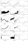 |
Fig. 1 Temporal evolution of semimajor axis (a), radial distance (r), eccentricity (e), orbital inclination (i), and the pericenter distance (q) of a long-lived NEO-Centaur for a period of 100 Myr (left), for the first 10 Myr of evolution (middle). The panels on the right highlight the effects of a single close encounter with Jupiter. |
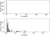 |
Fig. 2 Distribution of the residence time of NEO-Centaurs into the Centaur region (top). Zoom of the distribution up to approximately 500,000 years (bottom). |
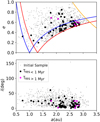 |
Fig. 3 Initial orbital distribution of 76 large NEOs that reached the Centaur region in the a × e (top) and a × i (bottom) planes, shown relative to the whole initial sample of large NEOs (gray dots). Black and pink dots highlight the NEOs that survived as NEO-Centaurs for residence times Tres < 1 Myr and Tres > 1 Myr, respectively. Blue and red lines denote the apocenter and pericenter lies of Earth and Mars, and the orange line denotes the apocenter of Jupiter. |
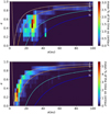 |
Fig. 4 Residence region for seven long-lived NEO-Centaurs (Tres > 1 Myr) (top) and sixty-nine short-lived NEO-Centaurs (Tres < 1 Myr) (bottom). The colored lines delineate the pericenter crossings of the giant planets’ orbits: Jupiter, Saturn, Uranus, and Neptune. The color code on the right indicates the mean percentage of time spent as a Centaur relative to the total lifetime of each subgroup in the (a × e) grid with ∆a = 2 au and ∆e = 0.1. |
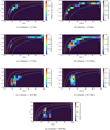 |
Fig. 5 Individual residence regions of the seven long-lived NEO-Centaurs. The colored lines delineate the pericenter crossings of the giant planets’ orbits: Jupiter, Saturn, Uranus, and Neptune. The color code on the right indicates the percentage each long-lived NEO-Centaur (Tres > 1 Myr) spends on the (a × e) grid, with ∆a = 2 au and ∆e = 0.1. |
6 Constraints on the current NEO-Centaur population
The estimated population of Centaurs larger than 1 km ranges from approximately 106 to 108 bodies (Di Sisto & Brunini 2007; Volk & Malhotra 2008). Based on the results of Liberato et al. (2023) (76 NEO-Centaurs), and on our simulations (115 NEOCentaurs), we estimate the fraction of NEO-Centaurs to be on the order of 10−4 and 10−2, corresponding to 0.01-1% of the presumable Centaur population larger than 1 km.
Currently, 983 Centaurs are known (NASA Jet Propulsion Laboratory 2026). Of the 58 Centaurs with estimated diameters, 12 measure less than 5 km, as shown in the top panel of Figure 7. The bottom panel of Figure 7 shows the size distribution of 839 NEOs with diameters greater than 1 km, together with 76 NEO-Centaurs. The largest NEO transported to the Centaur region has a diameter of approximately 5 km. Additionally, the NEO population is predicted to be mainly composed of bodies smaller than 1 km in diameter (Morbidelli et al. 2020; Granvik et al. 2018). Therefore, the NEO-Centaur population is expected to be dominated by bodies smaller than 5 km in diameter.
Figure 8 shows the orbital distribution of the 983 known Centaurs in the (a × e) grid, categorized by size. Most objects have unknown sizes (gray dots). Among those with determined sizes, some are larger than 5 km (purple dots) and others are smaller than 5 km (yellow dots).
The 13 known Centaurs with semimajor axes a < 10 au and eccentricities e > 0.4 could be considered plausible candidates for former NEOs that transitioned to the Centaur region. They are: 2010 LG61, 2014 KG2, 2010 HR68, 2010 LN101, 2010 NU12, 2010 CD201, 2010 EG4, 2010 BA101, 2010 JO142, 2010 DJ61, 2010 OM101, 2010 OR1, and 2010 CM53 (NASA Jet Propulsion Laboratory 2026).
Observational biases likely favor the detection of larger bodies beyond Saturn, resulting in an apparent scarcity of small Centaurs in this region.
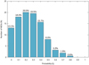 |
Fig. 6 Percentage distribution of 839 NEOs as a function of their probability to become Centaurs. |
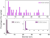 |
Fig. 7 Distribution of sizes for 58 Centaurs with estimated diameters (top) and of 839 NEOs with diameters greater than 1 km, along with 76 NEO-Centaurs (bottom). (NASA Jet Propulsion Laboratory 2026; European Space Agency 2025). |
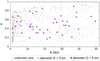 |
Fig. 8 Orbital distribution of known Centaurs in the (a × e) grid, categorized by size (NASA Jet Propulsion Laboratory 2026). |
7 Summary and final comments
This work investigates the transition of minor bodies from the inner Solar System into the Centaur region. The study by Liberato et al. (2023) considers a sample of 839 near-Earth objects (NEOs) with diameters larger than 1 km and finds that approximately 9% of the sample (76 objects) transition into NEO-Centaurs. We conducted a more detailed analysis that shows that seven of these initial NEOs became long-lived NEOCentaurs, surviving for more than 1 Myr in the Centaur region. In contrast, 69 NEOs became short-lived NEO-Centaurs, with a median residence time of 20 000 years. Overall, the average residence time of the NEO-Centaurs is 2.3 Myr, largely driven by the long-lived objects.
Near-Earth objects from the Amor and Apollo classes with higher eccentricity and lower inclination are more likely to move into Jupiter-family comets (JFCs) and subsequently reach the Centaur region. The short-lived NEO-Centaurs show random orbital evolution in the (a × e) grid, whereas the long-lived NEOCentaurs exhibit a less scattered evolution and remain largely within semimajor axis intervals.
The statistical analysis indicates a significant likelihood that NEOs are transported to the Centaur region. Of the 839 NEOs analyzed, only 13% exhibited zero probability of reaching the Centaur region. Approximately 63% of the NEOs, corresponding to 463 objects, fall within a probability range of 20-40%. In a more restrictive analysis, we estimate that 14% of the larger NEO population has a probability ≥50% of becoming NEO-Centaurs.
We infer that NEO-Centaurs constitute 0.01-1% of the population of Centaurs larger than 1 km and that the NEO-Centaur population is likely composed of bodies smaller than 5 km in diameter. Because the transport of NEOs to the Centaur region is feasible, minor bodies in the outer Solar System that show signs of space weathering may be detectable.
Minor airless bodies in the terrestrial region of the Solar System may undergo surface changes due to space weathering (Sergeyev et al. 2023; Simion et al. 2021; Rubino et al. 2020; Marchi et al. 2006, 2005; Binzel et al. 2004). Various phenomena, such as micrometeorite bombardment, radiation, solar wind, and cosmic rays, contribute to space weathering (Lantz et al. 2017; Pieters & Noble 2016; Shestopalov et al. 2013; Chapman 2004). There is no consensus on the timescale required for minor
bodies to exhibit signs of space weathering. Estimates suggest that asteroids that spend around 104−106 years at a heliocentric distance of 1 au may exhibit evidence of space weathering (Strazzulla et al. 2005). A more recent study estimates that at distances ≤1 au, these bodies require approximately 5 Myr to undergo such surface modification (Graves et al. 2019).
Some minor bodies in the outer Solar System may have previously passed through the inner Solar System. Identifying these objects introduces additional considerations that could influence future studies, particularly for observational astronomers. Evidence of inner objects within the outer Solar System has been found, as shown in Meech et al. (2016), which discusses the case of C/2014 S 3 (PANSTARRS), the first long-period comet exhibiting inner Solar System asteroid characteristics. As in the case of C/2014 S 3, our results suggest the existence of a population of minor bodies among the Centaurs that were once NEOs. These objects await detection.
Acknowledgements
This research was supported by resources supplied by the Center for Scientific Computing (NCC/GridUNESP) of the São Paulo State University (UNESP), for which we are grateful. We also acknowledge the support of the National Council for Scientific and Technological Development (CNPq) for grants 316991/2023-6 and 405349/2025-4, the São Paulo Research Foundation (FAPESP) for grant 2022/11783-5, as well as the project GaiaMoons of the Agence Nationale de Recherche (France), grant ANR-22-CE49-0002.
References
- Araujo, R., Galiazzo, M., Winter, O., & Sfair, R. 2018a, MNRAS, 476, 5323 [Google Scholar]
- Araujo, R., Winter, O., & Sfair, R. 2018b, MNRAS, 479, 4770 [Google Scholar]
- Araujo, R., Liberato, L., & Winter, O. C. 2023, EPJST, 232, 3023 [Google Scholar]
- Bailey, B. L., & Malhotra, R. 2009, Icarus, 203, 155 [Google Scholar]
- Binzel, R. P., Rivkin, A. S., Stuart, J. S., et al. 2004, Icarus, 170, 259 [NASA ADS] [CrossRef] [Google Scholar]
- Bottke Jr, W. F., Morbidelli, A., Jedicke, R., et al. 2002, Icarus, 156, 399 [NASA ADS] [CrossRef] [Google Scholar]
- Chambers, J. E. 1999, MNRAS, 304, 793 [Google Scholar]
- Chapman, C. R. 2004, Annu. Rev. Earth Planet. Sci., 32, 539 [CrossRef] [Google Scholar]
- Di Sisto, R. P., & Brunini, A. 2007, Icarus, 190, 224 [Google Scholar]
- Di Sisto, R. P., & Rossignoli, N. L. 2020, CMDA, 132, 36 [Google Scholar]
- Di Sisto, R. P., Brunini, A., & De Elia, G. 2010, A&A, 519, A112 [NASA ADS] [CrossRef] [EDP Sciences] [Google Scholar]
- Di Sisto, R. P., Ramos, X. S., & Gallardo, T. 2019, Icarus, 319, 828 [NASA ADS] [CrossRef] [Google Scholar]
- Duffard, R., Pinilla-Alonso, N., Santos-Sanz, P., et al. 2014, A&A, 564, A92 [NASA ADS] [CrossRef] [EDP Sciences] [Google Scholar]
- Emel’Yanenko, V., Asher, D., & Bailey, M. 2007, MNRAS, 381, 779 [Google Scholar]
- Emel’Yanenko, V., Asher, D., & Bailey, M. 2013, Earth Moon Planets, 110, 105 [Google Scholar]
- European Space Agency 2025, NEOCC, accessed: May 7, 2025 [Google Scholar]
- Fernández, J. A., Gallardo, T., & Brunini, A. 2002, Icarus, 159, 358 [CrossRef] [Google Scholar]
- Galiazzo, M. A., Wiegert, P., & Aljbaae, S. 2016, Ap&SS, 361, 1 [NASA ADS] [CrossRef] [Google Scholar]
- Galiazzo, M., Silber, E., & Dvorak, R. 2019, MNRAS, 482, 771 [Google Scholar]
- Gallardo, T. 2006, Icarus, 184, 29 [Google Scholar]
- Gladman, B., Michel, P., & Froeschlé, C. 2000, Icarus, 146, 176 [NASA ADS] [CrossRef] [Google Scholar]
- Granvik, M., Morbidelli, A., Jedicke, R., et al. 2018, Icarus, 312, 181 [CrossRef] [Google Scholar]
- Graves, K. J., Minton, D. A., Molaro, J. L., & Hirabayashi, M. 2019, Icarus, 322, 1 [NASA ADS] [CrossRef] [Google Scholar]
- Greenstreet, S., Ngo, H., & Gladman, B. 2012, Icarus, 217, 355 [CrossRef] [Google Scholar]
- Hahn, G., & Lagerkvist, C.-I. 1987, CM, 43, 285 [Google Scholar]
- Horner, J., Evans, N., & Bailey, M. 2004a, MNRAS, 354, 798 [Google Scholar]
- Horner, J., Evans, N., & Bailey, M. 2004b, MNRAS, 355, 321 [Google Scholar]
- Kaplan, M., Erece, O., Aslan, G., & Eker, Z. 2016, ASR, 58, 2407 [Google Scholar]
- Lantz, C., Brunetto, R., Barucci, M. A., et al. 2017, Icarus, 285, 43 [CrossRef] [Google Scholar]
- Liberato, L., Araújo, R., & Winter, O. 2023, EPJST, 232, 3007 [Google Scholar]
- Marchi, S., Brunetto, R., Magrin, S., Lazzarin, M., & Gandolfi, D. 2005, A&A, 443, 769 [NASA ADS] [CrossRef] [EDP Sciences] [Google Scholar]
- Marchi, S., Paolicchi, P., Lazzarin, M., & Magrin, S. 2006, Proc. IAU, 2, 239 [Google Scholar]
- Meech, K. J., Yang, B., Kleyna, J., et al. 2016, Sci. Adv., 2, e1600038 [NASA ADS] [CrossRef] [Google Scholar]
- Morbidelli, A., Bottke Jr, W., Froeschlé, C., & Michel, P. 2002, Asteroids III, 409 [Google Scholar]
- Morbidelli, A., Delbo, M., Granvik, M., et al. 2020, Icarus, 340, 113631 [NASA ADS] [CrossRef] [Google Scholar]
- NASA Jet Propulsion Laboratory 2026, Small-Body Database Query, accessed: January 30, 2026 [Google Scholar]
- Pieters, C. M., & Noble, S. K. 2016, J. Geophys. Res. Planets, 121, 1865 [CrossRef] [Google Scholar]
- Prialnik, D., Barucci, M. A., & Young, L. 2019, The Trans-Neptunian Solar System (Elsevier) [Google Scholar]
- Rubino, S., Lantz, C., Baklouti, D., et al. 2020, PSJ, 1, 61 [Google Scholar]
- Sergeyev, A., Carry, B., Marsset, M., et al. 2023, A&A, 679, A148 [NASA ADS] [CrossRef] [EDP Sciences] [Google Scholar]
- Shestopalov, D. I., Golubeva, L. F., & Cloutis, E. A. 2013, Icarus, 225, 781 [NASA ADS] [CrossRef] [Google Scholar]
- Shoemaker, E. M., & Helin, E. F. 1978, NASA, Washington Asteroids [Google Scholar]
- Simion, N., Popescu, M., Licandro, J., et al. 2021, MNRAS, 508, 1128 [Google Scholar]
- Strazzulla, G., Dotto, E., Binzel, R., et al. 2005, Icarus, 174, 31 [CrossRef] [Google Scholar]
- Tancredi, G. 1998, CMDA, 70, 181 [Google Scholar]
- Tiscareno, M. S., & Malhotra, R. 2003, AJ, 126, 3122 [NASA ADS] [CrossRef] [Google Scholar]
- Volk, K., & Malhotra, R. 2008, AJ, 687, 714 [Google Scholar]
- Wood, J., & Horner, J. 2015, arXiv preprint [arXiv:1503.06096] [Google Scholar]
All Figures
|
Fig. 1 Temporal evolution of semimajor axis (a), radial distance (r), eccentricity (e), orbital inclination (i), and the pericenter distance (q) of a long-lived NEO-Centaur for a period of 100 Myr (left), for the first 10 Myr of evolution (middle). The panels on the right highlight the effects of a single close encounter with Jupiter. |
| In the text | |
|
Fig. 2 Distribution of the residence time of NEO-Centaurs into the Centaur region (top). Zoom of the distribution up to approximately 500,000 years (bottom). |
| In the text | |
|
Fig. 3 Initial orbital distribution of 76 large NEOs that reached the Centaur region in the a × e (top) and a × i (bottom) planes, shown relative to the whole initial sample of large NEOs (gray dots). Black and pink dots highlight the NEOs that survived as NEO-Centaurs for residence times Tres < 1 Myr and Tres > 1 Myr, respectively. Blue and red lines denote the apocenter and pericenter lies of Earth and Mars, and the orange line denotes the apocenter of Jupiter. |
| In the text | |
|
Fig. 4 Residence region for seven long-lived NEO-Centaurs (Tres > 1 Myr) (top) and sixty-nine short-lived NEO-Centaurs (Tres < 1 Myr) (bottom). The colored lines delineate the pericenter crossings of the giant planets’ orbits: Jupiter, Saturn, Uranus, and Neptune. The color code on the right indicates the mean percentage of time spent as a Centaur relative to the total lifetime of each subgroup in the (a × e) grid with ∆a = 2 au and ∆e = 0.1. |
| In the text | |
|
Fig. 5 Individual residence regions of the seven long-lived NEO-Centaurs. The colored lines delineate the pericenter crossings of the giant planets’ orbits: Jupiter, Saturn, Uranus, and Neptune. The color code on the right indicates the percentage each long-lived NEO-Centaur (Tres > 1 Myr) spends on the (a × e) grid, with ∆a = 2 au and ∆e = 0.1. |
| In the text | |
|
Fig. 6 Percentage distribution of 839 NEOs as a function of their probability to become Centaurs. |
| In the text | |
|
Fig. 7 Distribution of sizes for 58 Centaurs with estimated diameters (top) and of 839 NEOs with diameters greater than 1 km, along with 76 NEO-Centaurs (bottom). (NASA Jet Propulsion Laboratory 2026; European Space Agency 2025). |
| In the text | |
|
Fig. 8 Orbital distribution of known Centaurs in the (a × e) grid, categorized by size (NASA Jet Propulsion Laboratory 2026). |
| In the text | |
Current usage metrics show cumulative count of Article Views (full-text article views including HTML views, PDF and ePub downloads, according to the available data) and Abstracts Views on Vision4Press platform.
Data correspond to usage on the plateform after 2015. The current usage metrics is available 48-96 hours after online publication and is updated daily on week days.
Initial download of the metrics may take a while.