| Issue |
A&A
Volume 708, April 2026
|
|
|---|---|---|
| Article Number | L21 | |
| Number of page(s) | 5 | |
| Section | Letters to the Editor | |
| DOI | https://doi.org/10.1051/0004-6361/202659586 | |
| Published online | 24 April 2026 | |
Letter to the Editor
Ultra-fast simulations of the solar dipole and open flux
Space Physics and Astronomy Research Unit, University of Oulu, POB 8000, FI-90014 Oulu, Finland
★ Corresponding author: This email address is being protected from spambots. You need JavaScript enabled to view it.
Received:
24
February
2026
Accepted:
12
April
2026
Abstract
Context. The solar dipole captures important information characterizing the large-scale solar magnetic field. The evolution of the solar magnetic field including the solar dipole can be simulated with a surface flux transport (SFT) model, but these simulations are more extensive than is otherwise necessary to produce the evolution of the dipole alone.
Aims. We present a dipole flux transport (DFT) matrix method that combines the classic SFT model with dipole vector representation of the solar magnetic field, which enables significantly faster simulations of the solar dipole.
Methods. By simulating the evolution of basis vectors of a synoptic map, we were able to construct propagator matrices that produce the time evolution of the solar magnetic field by means of matrix multiplication. The computational speedup was achieved by compressing the propagator matrices to very small fraction (< 10−4) of their original size with a recent vector sum method.
Results. Depending on the time resolution, the DFT performs 100−1000 times faster than a 4-year SFT simulation of a single active region, while producing equivalent results. For multiple source regions, daily propagation matrices are sufficient to produce results that agree within 1% with the SFT simulation of solar cycle 24, while performing 80 times faster. If the evolution of individual active regions is needed, the DFT is equipped to perform 50000 times faster than the SFT model.
Conclusions. Overall, DFT makes solar dipole simulations extremely fast, making it possible to run thousands of simulations in a few minutes with a basic laptop setup. As the magnitude of the dipole vector closely matches the open solar flux (OSF) from the potential field source surface model, the DFT can be used to study the development of OSF in various scenarios in an extremely efficient way.
Key words: Sun: activity / Sun: corona / Sun: magnetic fields / Sun: photosphere
© The Authors 2026
 Open Access article, published by EDP Sciences, under the terms of the Creative Commons Attribution License (https://creativecommons.org/licenses/by/4.0), which permits unrestricted use, distribution, and reproduction in any medium, provided the original work is properly cited.
This article is published in open access under the Subscribe to Open model. This email address is being protected from spambots. You need JavaScript enabled to view it. to support open access publication.
1. Introduction
The evolution of the solar magnetic field is routinely simulated using surface flux transport (SFT) models (for a recent review and references, see Yeates et al. 2023). For certain applications, it is not necessary to retain all the information on the simulated photospheric magnetic field, whereby approximating the magnetic field as a global dipole is sufficient. In particular, the axial dipole moment of the Sun has been studied extensively because its strength around the solar minimum correlates quite well with the amplitude of the subsequent solar cycle (Upton & Hathaway 2014; Cameron et al. 2016; Iijima et al. 2017; Jiang et al. 2018; Whitbread et al. 2018; Yeates 2020; Petrovay et al. 2020). More generally, the solar dipole is also relevant to studies of coronal and heliospheric magnetic fields because the higher order multipoles fall off rapidly with height (Wang 2009). For example, the equatorial dipole moment has been shown to play an important role in shaping the heliospheric magnetic field (Wang et al. 2000a,b; Wang & Sheeley 2003). This, in turn, modulates the propagation of cosmic rays in the heliosphere (Jokipii & Thomas 1981).
In certain situations, SFT calculations can be simplified or even avoided entirely by considering the symmetries of the problem. When the quantity of interest is the axial dipole moment, the full 2D simulation can be reduced to a 1D simulation, since the axial dipole solely depends on the longitudinally averaged field (DeVore et al. 1984; Cameron & Schüssler 2007; Iijima et al. 2017; Petrovay & Talafha 2019; Yeates 2020). Furthermore, if only the asymptotic behavior of the axial dipole moment is required, SFT calculations can be replaced by an algebraic approach (Petrovay et al. 2020; Wang et al. 2021). This method maps the magnetic field of an active region to its asymptotic axial dipole moment, exploiting the fact that in SFT simulations, the field approaches a steady state where the magnetic flux is confined to polar regions. The asymptotic axial dipole moment of an active region can be expressed as the initial axial dipole strength multiplied by an amplification factor. For bipolar magnetic regions (BMRs), this factor is a Gaussian function of latitude alone, but the method can be generalized to arbitrary flux distributions (Jiang et al. 2014; Petrovay et al. 2020; Wang et al. 2021; Talafha et al. 2022; Yeates et al. 2023). Furthermore, because the SFT model is linear, individual contributions can be summed to obtain the total axial dipole moment. In contrast, Tähtinen et al. (2026), who studied the evolution of the equatorial rather than the axial dipole, avoided performing > 105 SFT simulations by rotating the solutions of previously simulated active regions in longitude. Due to the linearity and longitudinal symmetry of the SFT model, these rotated solutions are equivalent to simulations with correspondingly rotated source regions.
The strength of the solar dipole is typically modeled with solar dipole moment corresponding to l = 1 term in a spherical harmonic expansion. Recently, Tähtinen et al. (2024, 2026) developed an alternative way for describing the solar dipole. Their vector sum method produces a vector which shares orientation with the traditional dipole, but whose magnitude has units of magnetic flux and equals the total photospheric magnetic flux aligned with the dipole axis. Importantly, the magnitude of this dipole vector closely matches with the open solar flux (OSF) from the potential field source surface (PFSS) model (Altschuler & Newkirk 1969; Schatten et al. 1969; Wang & Sheeley 1992) with a standard source surface radius of 2.5 R⊙. This result directly relates the total magnetic flux escaping from the Sun (i.e., OSF) to the photospheric magnetic flux distribution (at least in the context of PFSS modeling).
In this Letter, we show how the vector sum method of Tähtinen et al. (2024, 2026) can be combined with a classic SFT model to construct a propagator matrix that maps the initial magnetic field of a synoptic map to a dipole vector at a later time. We refer to this matrix method as dipole flux transport (DFT) as it describes the evolution of the solar dipole vector under the dynamics of the SFT model. DFT offers a speedup of up to four orders of magnitude in our test cases, which were set up to address various problems in solar dipole modeling. As the magnitude of the dipole vector offers a close match with the OSF from the PFSS model, the method also provides a way to study the development of OSF extremely efficiently.
2. Data
We compared the performance of the DFT to the SFT model by simulating the evolution of solar cycle 24. We used the pole-filled synoptic maps of the radial magnetic field (hmi.synoptic_mr_polfil_720s) from the Helioseismic and Magnetic Imager on board the Solar Dynamics Observatory (SDO/HMI; Scherrer et al. 2012; Pesnell et al. 2012) and the active region database derived from Spaceweather HMI Active Region Patch data (SHARP; Bobra et al. 2014) using an open-source Python code1 described in Yeates (2020). This algorithm transforms HMI SHARPS into uniform sine-latitude and longitude grid and removes active regions with high flux imbalance. Active regions that are recognized as remnants of regions observed in previous rotation are also removed. Data covers Carrington rotations 2097–2224 (May 2010 to December 2019) that correspond to solar cycle 24. Altogether there are 1095 active regions.
3. Dipole flux transport
Our aim is to construct a propagator matrix that represents the evolution of the solar dipole vector under the dynamics of the SFT model described in Appendix A. The idea is to first construct the propagator M for the full SFT simulation, which turns the SFT simulation into matrix multiplication,
 (1)
(1)
where the propagator M(t) maps the initial magnetic field, B0, to the final magnetic field, B, at time t. The matrix M is inconveniently large for offering a significant speedup for full SFT simulations, but its size can be reduced by four orders of magnitude using the vector sum method described in Appendix B. This compactified matrix can then be used to simulate the time evolution of the solar dipole as
 (2)
(2)
where V represents the vector sum matrix that maps the full synoptic map into a dipole vector D. Matrix VM then represents the propagator that maps the initial magnetic field, B0, to dipole vector, D, at some later time t. Next we show in detail how to construct the propagator matrix VM.
3.1. Propagator for the surface flux transport
Let Eij denote a matrix unit which has only one nonzero value with a value of 1 in the ith row and jth column. These matrix units, Eij, correspond to standard basis vectors of synoptic map. A full synoptic map can then be written as
 (3)
(3)
where Bij denotes the magnetic field strength of the ith row and the jth column of a synoptic map B. Now, let ℳ(B0; t) denote the operator for SFT simulation. This is a linear operator that takes in a synoptic map and evolves it to time t, so that the magnetic field at time t is B(t) = ℳ(B0; t), where B0 is the initial synoptic map. Now, due to the linearity, we have
 (4)
(4)
This equation shows that instead of simulating the evolution of the magnetic field with the SFT model, we can simulate the evolution of a set of matrix units, Eij, scale these simulations with the initial magnetic field values, B0ij, and, finally, sum these together to produce the time evolution for the full synoptic map. The advantage is that the matrix units need to be simulated only once and the resulting matrices can then be used to simulate the evolution of any synoptic map with the time resolution that was used to calculate ℳ(Eij; t).
If, as often is, the synoptic map has 180 × 360 = 64800 pixels, a general situation would require as many SFT simulations to produce the required ℳ(Eij; t) matrices. However, the equations of the SFT model described in Appendix A have a considerable redundancy because of the large-scale flows that are both axisymmetric and antisymmetric across the equator. For this reason, we only need to use the SFT model to simulate ℳ(Eij; t) matrices for a single longitude of one hemisphere, which reduces the number of required SFT simulations down to 90. All the remaining ℳ(Eij; t) matrices can then be obtained via longitudinal translations and/or mirroring across the equator from this core set of 90. Together the full set of ℳ(Eij; t) matrices corresponds to the matrix M(t) in Eqs. (1) and (2).
Let B0 and B denote the vectorized versions of the initial and final synoptic maps and M(t) a matrix whose columns are equal to vectorized versions of ℳ(Eij; t) matrices. Equation (4) can then be expressed as matrix multiplication via Eq. (1). The matrix M(t) depends on time step used to create matrix unit responses ℳ(Eij; t).
The feasibility of the propagator approach depends on the size of the matrix M. It is a square matrix whose linear size equals the number of pixels in a synoptic map. For a typical 180 × 360 synoptic map, the size of M is 64800 × 64800, which takes more than 30 Gb to store in memory. In practice, it is not necessarily efficient (or even possible) to calculate the matrix product in single step and the calculation needs to be carried in parts. For our laptop setup, the calculation of this matrix product takes about the time of SFT simulation lasting two Carrington rotations. Next, we show how the vector sum can be used to significantly reduce the dimensions of M, producing a matrix that represents the evolution of the solar dipole evolving under the SFT model.
3.2. Propagator for the dipole flux transport
Let 𝒱(B) denote the operator for the vector sum operation described in Appendix B. It is a linear operator that takes a synoptic map, B, and produces a three-component vector, V, describing the magnitude and orientation of the solar dipole. Now, due to the linearity of 𝒱 and ℳ the dipole vector at time t can be calculated as
 (5)
(5)
which corresponds to the matrix product of Eq. (2). Equation (5) shows that to produce the evolution of the dipole vector, we do not need the full matrix M and it suffices to work with more compact propagation matrix VM. We can obtain the matrix VM directly by calculating the vector sums of ℳ(Eij; t) matrix unit responses. For 180 × 360 synoptic map, the size of VM is 3 × 64800, which decreases the number of stored components by a factor of 21600.
Since the multiplication by the matrix VM(t) maps the synoptic map to dipole vector at single time t, it is practical to produce a set of matrices VM(t), such that t ∈ {t1, …, tn}. This is straightforward to achieve as matrices corresponding to different timesteps can be created during the same SFT simulation. We computed the VM(t) matrices with daily and Carrington resolution up to 11 years. Since the propagator matrices VM(t) describe the evolution of solar dipole under the dynamics of the SFT model, we refer to method of simulating the solar dipole with Eq. (2) as the dipole flux transport (DFT).
4. Applications
Here, we compare the performance of the DFT and SFT simulations in a few different scenarios. All simulations were performed on a Lenovo ThinkPad P52 laptop from 2019 equipped with an Intel Core i7-8750H CPU, 32 GB RAM, running Windows 11. The computations were carried out using MATLAB R2022b without parallelization. We measured the performance using MATLAB’s timeit function, which essentially reports the median runtime of 10 simulation runs. Table 1 gives runtimes for the SFT and DFT simulations for different scenarios. In the last two rows, the SFT runtimes are estimated from the solar cycle 24 SFT simulation, as running them in full would require excessive computation time. The propagation matrices and code for running the following tests are available on GitHub2.
Runtimes of different simulation scenarios.
4.1. Evolution of active regions
The simplest and most straightforward application is the evolution of single map without any flux emergence. Such simulations are useful, for example, for studying how the properties of the active regions affect their evolution. The runtime of the DFT simulation depends on the number of nonzero pixels, as we only need to compute their time evolution. Because the runtime of the DFT depends on number of nonzero pixels in initial map, we selected the largest active region of solar cycle 24 corresponding to NOAA 12192 to obtain the estimate for the upper bound of the runtime of the DFT simulation. We ran the simulation for four years, which is enough time for the nonaxisymmetric magnetic field to annihilate and magnetic field to settle into an asymptotic axial dipole state (see, e.g., Wang & Sheeley 2002).
With a Carrington resolution, a 4-year (54 rotations) DFT simulation of an active region takes 0.09 seconds. DFT speeds up the calculation by a factor of 2982 when compared to SFT simulation of the same length that takes 259.41 seconds. Increasing the time resolution slows down the matrix calculation in a roughly linear manner and, with the daily resolution, the similar 4-year simulation takes 2.18 seconds. Even with the daily resolution, the DFT performs 119 times faster than the SFT.
4.2. Evolution of solar cycle
DFT can also be applied to multiple active regions. To do so, the evolution of each active region and the initial magnetic field needs to be simulated independently. Each simulation produces a vector timeseries that, when summed together, produce the evolution of the full dipole vector of the solar magnetic field. For this summation to make sense, the time resolution needs to be sufficiently high so that the individual timeseries, which have different initial starting points, can be lined up together. For global simulations of the solar magnetic field which typically have a time resolution of one Carrington resolution, a 1 day resolution for individual simulations seems a reasonable choice. Since the evolution of each active region needs to be simulated separately, the cost of such simulations grows with the number of active regions.
The upper panel of Fig. 1 compares the dipole vector magnitude between the DFT and the SFT simulations for Carrington rotations 2097−2224. The Pearson correlation between the two methods is 0.999994. The lower panel shows that the relative difference between the DFT and the SFT simulation is at most 1%. The DFT simulation takes only 7.48 seconds in our tests, thereby outperforming SFT simulations (lasting 608.16 seconds) by factor of 81.
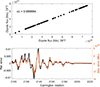 |
Fig. 1. Comparison of SFT and DFT simulations. Upper panel: Scatter plot showing the dipole vector magnitude from the DFT (y-axis) and from the SFT (x-axis) simulation. Lower panel: Relative (black) and absolute (orange) error of the DFT dipole vector magnitude. |
For some applications, it is useful to have the time evolution of individual active regions (e.g., Yeates 2020; Tähtinen et al. 2026), which the DFT simulation gives for free. In this case, we estimate that the DFT performs 54982 times faster than the SFT model, which would take about 4.76 days because the evolution of each of the 1095 active regions needs to be simulated separately.
4.3. Ensemble predictions
A natural application of the DFT model is probabilistic ensemble modeling. Consider an ensemble forecast based on active regions generated by a probabilistic model and evaluated against HMI observations from solar cycle 24. For such a hindcast, one would generate an ensemble of N realizations and evolve the magnetic field forward by a time Δt, starting from each Carrington rotation between CR2097 and CR2224. Assuming that the average number and timing of active regions match those observed, HMI SHARPs can be used to estimate the runtime of such predictions. For a single 180-day hindcast, the median runtime is 0.74 seconds for the DFT model and 4103 seconds for the SFT model. For N = 100, this amounts to about one minute for the DFT and more than 4.5 days for the SFT simulation.
5. Discussion
The DFT model presented in this Letter allows us to simulate the evolution of the solar dipole extremely efficiently. This is possible for two reasons. First, the linearity of the classic SFT model allows us to precompute the propagation matrices that capture the dynamics of the SFT model, thereby allowing us to turn the SFT simulation into matrix product. Second, the significant speedup of computations is achieved by using the vector sum to compress the size of propagation matrices by a factor of 21600.
For a single map (e.g., active region), the DFT provides numerically identical results with the SFT model at the time resolution of the propagation matrix. The DFT can also be used to model the evolution of the solar dipole subject to multiple source regions emerging at different times. In our tests, daily resolution propagation matrix is enough to produce results that agree with Carrington resolution SFT simulation with a maximum relative error of around 1%. Compared to earlier methods used to speed up the simulations of the solar dipole (DeVore et al. 1984; Cameron & Schüssler 2007; Iijima et al. 2017; Petrovay & Talafha 2019; Yeates 2020; Petrovay et al. 2020; Wang et al. 2021; Tähtinen et al. 2026), the DFT produces the evolution of the full dipole vector, not just its axial component. In addition, it works for arbitrary initial conditions.
DFT shares the same limitations as the SFT model from which it was derived and cannot account for nonlinear processes, such as reduced effective diffusivity in regions of strong magnetic field. In principle, DFT can be applied to time-dependent scenarios (e.g., varying meridional flow amplitude), but this could turn out to be rather cumbersome because the propagator matrices become path-dependent.
Despite its simplicity, the solar dipole contains a lot of crucial information about the large-scale magnetic field, thereby making the efficient simulations highly useful. The speedup is greatest in situations that demand many individual simulations. For example, Tähtinen et al. (2026) simulated the evolution of individual active regions to quantify their effect on the large-scale dipole. With the DFT, this calculation is 1000 times faster than their calculation, which was done parallel on a computer cluster with 40 cores. Another context where the DFT is likely to prove useful is ensemble modeling. For example, given a generative active region model (see, e.g., Jha & Upton 2024), the DFT can be used for probabilistic ensemble modeling extremely efficiently. In addition, as the magnitude of the dipole vector closely matches the PFSS OSF (Tähtinen et al. 2024), the development of OSF can be studied in various scenarios with a nearly negligible computational cost.
6. Conclusions
We have developed a DFT matrix method to simulate the evolution of the solar dipole up to 50000 times faster than regular SFT simulations. Importantly, the method provides the full dipole vector, greatly increasing the scope of dipole simulations, which have thus far been limited to the axial dipole component. We anticipate that the DFT will prove especially useful for ensemble methods to study solar activity. It can also be used to study the development of OSF extremely efficiently in various scenarios.
Acknowledgments
I.T. and T.A. acknowledge the financial support by the Research Council of Finland to the SOLEMIP (project no. 357249). We thank the anonymous referee for their constructive comments. The authors wish to acknowledge CSC – IT Center for Science, Finland, for computational resources.
References
- Altschuler, M. D., & Newkirk, G. 1969, Sol. Phys., 9, 131 [NASA ADS] [CrossRef] [Google Scholar]
- Bobra, M. G., Sun, X., Hoeksema, J. T., et al. 2014, Sol. Phys., 289, 3549 [Google Scholar]
- Cameron, R., & Schüssler, M. 2007, ApJ, 659, 801 [Google Scholar]
- Cameron, R. H., Jiang, J., & Schüssler, M. 2016, ApJ, 823, L22 [Google Scholar]
- DeVore, C. R., Boris, J. P., & Sheeley, N. R., Jr. 1984, Sol. Phys., 92, 1 [NASA ADS] [CrossRef] [Google Scholar]
- Iijima, H., Hotta, H., Imada, S., Kusano, K., & Shiota, D. 2017, A&A, 607, L2 [NASA ADS] [CrossRef] [EDP Sciences] [Google Scholar]
- Jha, B. K., & Upton, L. A. 2024, ApJ, 962, L15 [NASA ADS] [CrossRef] [Google Scholar]
- Jiang, J., Cameron, R. H., & Schüssler, M. 2014, ApJ, 791, 5 [Google Scholar]
- Jiang, J., Wang, J.-X., Jiao, Q.-R., & Cao, J.-B. 2018, ApJ, 863, 159 [NASA ADS] [CrossRef] [Google Scholar]
- Jokipii, J. R., & Thomas, B. 1981, ApJ, 243, 1115 [NASA ADS] [CrossRef] [Google Scholar]
- Pesnell, W. D., Thompson, B. J., & Chamberlin, P. C. 2012, Sol. Phys., 275, 3 [Google Scholar]
- Petrovay, K., & Talafha, M. 2019, A&A, 632, A87 [NASA ADS] [CrossRef] [EDP Sciences] [Google Scholar]
- Petrovay, K., Nagy, M., & Yeates, A. R. 2020, J. Space Weather Space Clim., 10, 50 [EDP Sciences] [Google Scholar]
- Schatten, K. H., Wilcox, J. M., & Ness, N. F. 1969, Sol. Phys., 6, 442 [Google Scholar]
- Scherrer, P. H., Schou, J., Bush, R. I., et al. 2012, Sol. Phys., 275, 207 [Google Scholar]
- Snodgrass, H. B., & Ulrich, R. K. 1990, ApJ, 351, 309 [NASA ADS] [CrossRef] [Google Scholar]
- Tähtinen, I., Asikainen, T., & Mursula, K. 2024, A&A, 688, L32 [NASA ADS] [CrossRef] [EDP Sciences] [Google Scholar]
- Tähtinen, I., Asikainen, T., & Mursula, K. 2026, A&A, 706, A235 [NASA ADS] [CrossRef] [EDP Sciences] [Google Scholar]
- Talafha, M., Nagy, M., Lemerle, A., & Petrovay, K. 2022, A&A, 660, A92 [NASA ADS] [CrossRef] [EDP Sciences] [Google Scholar]
- Upton, L., & Hathaway, D. H. 2014, ApJ, 780, 5 [Google Scholar]
- Wang, Y. M. 2009, Space Sci. Rev., 144, 383 [NASA ADS] [CrossRef] [Google Scholar]
- Wang, Y. M., & Sheeley, N. R., Jr. 1992, ApJ, 392, 310 [NASA ADS] [CrossRef] [Google Scholar]
- Wang, Y.-M., & Sheeley, N. R. 2002, J. Geophys. Res.: Space Phys., 107, 1302 [NASA ADS] [Google Scholar]
- Wang, Y. M., & Sheeley, N. R., Jr. 2003, ApJ, 590, 1111 [Google Scholar]
- Wang, Y. M., Lean, J., & Sheeley, N. R., Jr. 2000a, Geophys. Res. Lett., 27, 505 [NASA ADS] [CrossRef] [Google Scholar]
- Wang, Y. M., Sheeley, N. R., Jr., & Lean, J. 2000b, Geophys. Res. Lett., 27, 621 [Google Scholar]
- Wang, Z.-F., Jiang, J., & Wang, J.-X. 2021, A&A, 650, A87 [NASA ADS] [CrossRef] [EDP Sciences] [Google Scholar]
- Whitbread, T., Yeates, A. R., & Muñoz-Jaramillo, A. 2018, ApJ, 863, 116 [NASA ADS] [CrossRef] [Google Scholar]
- Yeates, A. R. 2020, Sol. Phys., 295, 119 [Google Scholar]
- Yeates, A. R., Cheung, M. C. M., Jiang, J., Petrovay, K., & Wang, Y.-M. 2023, Space Sci. Rev., 219, 31 [CrossRef] [Google Scholar]
Appendix A: Surface flux transport
The classic SFT model (see, e.g., Yeates et al. 2023) describes the evolution of the radial magnetic field subject to differential rotation, Ω(θ), meridional flow, uθ(θ), and turbulent diffusion, η, with the induction equation,
 (A.1)
(A.1)
where uh describes the horizontal flow velocity (due to Ω(θ) and uθ(θ)) and the magnetic flux emergence is modeled with the source term, S. The explicit form of the governing equation is
 (A.2)
(A.2)
In this Letter, we adopt the differential rotation profile of Snodgrass & Ulrich (1990), expressed as
![Mathematical equation: $$ \begin{aligned} \Omega (\theta ) = 0.18 - 2.396 \cos ^2(\theta ) - 1.787 \cos ^4(\theta ) \quad [^{\circ }\mathrm{day}^{-1}], \end{aligned} $$](/articles/aa/full_html/2026/04/aa59586-26/aa59586-26-eq8.gif) (A.3)
(A.3)
and the meridional flow profile of Whitbread et al. (2018), expressed as
 (A.4)
(A.4)
with their shape parameter being p = 2.33. We set the diffusivity to η = 350 km2/s and the meridional flow amplitude to u0 = 11 m/s, for which Tähtinen et al. (2026) found the best-fit values for solar cycle 24, using the total vector sum as the optimization metric.
Appendix B: Vector sum and solar dipole
The solar dipole can be efficiently represented using the recent vector sum method (Tähtinen et al. 2024, 2026). In the vector sum method, the pixels of a synoptic magnetogram are represented as vectors in heliographic spherical coordinates. The length of each vector corresponds to the total magnetic flux within the magnetogram pixel and the direction to the location of the pixel on the solar surface. The vector sum is then straightforwardly a sum of these spherical vectors producing a single vector describing the orientation and strength of the solar dipole. The orientation of the dipole vector equals the orientation of the first multipole (dipole) in the spherical harmonic expansion, but its magnitude differs from the solar dipole moment by a factor of  and it has units of flux instead of flux density.
The magnitude of the dipole vector closely matches the open solar flux (OSF) derived from the potential field source surface (PFSS) model with a source surface radius Rss = 2.5 R⊙. Furthermore, Tähtinen et al. (2026) showed that the magnitude of the dipole vector equals the photospheric magnetic flux aligned with the dipole axis, thus relating PFSS OSF directly to the distribution of the magnetic fields in the photosphere.
All Tables
All Figures
|
Fig. 1. Comparison of SFT and DFT simulations. Upper panel: Scatter plot showing the dipole vector magnitude from the DFT (y-axis) and from the SFT (x-axis) simulation. Lower panel: Relative (black) and absolute (orange) error of the DFT dipole vector magnitude. |
| In the text | |
Current usage metrics show cumulative count of Article Views (full-text article views including HTML views, PDF and ePub downloads, according to the available data) and Abstracts Views on Vision4Press platform.
Data correspond to usage on the plateform after 2015. The current usage metrics is available 48-96 hours after online publication and is updated daily on week days.
Initial download of the metrics may take a while.