| Issue |
A&A
Volume 708, April 2026
|
|
|---|---|---|
| Article Number | A331 | |
| Number of page(s) | 11 | |
| Section | Planets, planetary systems, and small bodies | |
| DOI | https://doi.org/10.1051/0004-6361/202558830 | |
| Published online | 22 April 2026 | |
Thermal variability driven by gravity waves in Triton's atmosphere
1
State Key Laboratory of Lunar and Planetary Sciences, Macau University of Science and Technology,
Taipa
999078,
Macao,
PR China
2
CNSA Macau Center for Space Exploration and Science,
Taipa
999078,
Macao,
PR China
3
Planetary Environment and Astrobiological Research Laboratory (PEARL), School of Atmospheric Sciences, Sun Yat-sen University,
Zhuhai
519082,
PR China
★ Corresponding author: This email address is being protected from spambots. You need JavaScript enabled to view it.
Received:
31
December
2025
Accepted:
17
March
2026
Abstract
Context. The thermal structure of Triton’s upper atmosphere has been recognized to be primarily influenced by magnetospheric electron precipitation and solar extreme ultraviolet (EUV) radiation. Gravity waves (GWs) may also act as an important mechanism for redistributing thermal energy, although they have not been directly observed in Triton’s atmosphere. Potential sources of GWs include geyser-like plumes near the surface, energetic particle deposition, and solar radiation.
Aims. This study aims to investigate the effects of GWs on the thermal variations in Triton’s upper atmosphere. We investigated the propagation and dissipation of waves with different horizontal wavelengths and phase speeds, and their impacts on the thermospheric temperature structure.
Methods. We used a linear full-wave model, in which a Gaussian source is introduced to represent waves excited by geyser-like plumes near the surface. The model examines wave propagation and dissipation over a broad range of temporal and spatial scales and evaluates the resulting heating and cooling effects on the background atmosphere.
Results. Our simulations indicate that GWs propagate adiabatically in the lower atmosphere, with density and temperature perturbations anti-phased and with horizontal and vertical velocities in phase. Wave dissipation due to molecular viscosity and thermal conduction occurs in the upper atmosphere, resulting in phase shifts between temperature, density, and velocity perturbations. Wave amplitudes increase with horizontal wavelength and phase speed, with peak amplitudes occurring below 200 km for short-wavelength low-phase speed modes and reaching altitudes of up to 300 km for long-wavelength high-phase speed modes. The maximum temperature and density perturbations are below 5% for short-wavelength modes but increase to nearly 10% for waves with longer horizontal wavelengths. Wave-induced heating is dominated by the sensible heat flux, leading to heating in the lower atmosphere and cooling in the upper atmosphere, with rates on the order of 10−10 erg cm−3 s−1 and an associated energy flux of up to 10−3 erg cm−2 s−1. The associated temperature increase at the exobase ranges from a few kelvins to several tens of kelvins, depending on the horizontal wavelength, and is comparable to heating from solar EUV radiation and magnetospheric particle precipitation.
Conclusions. This study demonstrates that GWs play a critical role in modulating the thermal structure of Triton’s upper atmosphere.
Key words: waves / planets and satellites: atmospheres / planets and satellites: individual: Triton
© The Authors 2026
 Open Access article, published by EDP Sciences, under the terms of the Creative Commons Attribution License (https://creativecommons.org/licenses/by/4.0), which permits unrestricted use, distribution, and reproduction in any medium, provided the original work is properly cited.
This article is published in open access under the Subscribe to Open model. This email address is being protected from spambots. You need JavaScript enabled to view it. to support open access publication.
1 Introduction
Triton, the largest satellite of Neptune, is regarded as a representative object of Kuiper Belt bodies and possesses a predominantly N2 atmosphere (Broadfoot et al. 1989). Previous studies have suggested that the thermal structure of Triton's thermosphere is primarily governed by magnetospheric electron precipitation and solar extreme ultraviolet (EUV) radiation, with heating rates on the order of 10−10 erg cm−3 s−1 at altitudes of several hundred kilometers (km) (e.g., Stevens et al. 1992; Lyons et al. 1992; Krasnopolsky et al. 1993; Sittler & Hartle 1996; Strobel & Zhu 2017; Benne et al. 2024). Magnetospheric ion precipitation has also been shown to play an important role in the upper atmospheric energy deposition and ionization processes on Triton (Huang et al. 2025), and atmospheric and ionospheric chemistry can drive significant nonthermal escape from the upper atmosphere (Gu et al. 2021). However, the contribution of wave-induced heating to thermal variations in the upper atmosphere has not been adequately investigated. The aim of this study is to examine the role of atmospheric gravity waves (GWs) in modulating the thermal structure of Triton’s upper atmosphere.
Gravity waves are generated when air parcels are displaced from their equilibrium positions by external perturbations, with restoring forces provided by pressure gradients, buoyancy, and gravity (Väisälä 1925; Brunt 1927; Nappo 2002). It is well recognized that GWs transport and redistribute momentum and energy during their vertical propagation and dissipation in stratified atmospheres. These processes ultimately lead to momentum deposition associated with wave saturation and breaking, thereby modifying atmospheric circulation (e.g., Lindzen 1981; Holton 1983; Fritts 1984; Fritts & Alexander 2003; Yiğit et al. 2008; Medvedev & Yiğit 2019). GWs also play an important role in the energy balance of the middle and upper atmosphere (e.g., Walterscheid 1981; Yiğit & Medvedev 2009, 2012, 2015; Yiğit et al. 2012, 2014; Medvedev et al. 2023; Navarro & Schubert 2024). In addition, GW-induced processes have been linked to migrating diurnal tides (e.g., Yiğit & Medvedev 2017), ionospheric disturbances (e.g., Hines 1960; Yeh & Liu 1974; Tripathi et al. 2023; Wang et al. 2023), the formation of CO2 ice clouds on Mars (e.g., Yiğit et al. 2015, 2018), thermal structure variations in the Martian thermosphere and atmospheric escape (e.g., Medvedev & Yiğit 2012; Yiğit et al. 2021; Gu et al. 2024), thermospheric structures of Jupiter and Saturn (e.g., French & Gierasch 1974; Barrow & Matcheva 2011, 2013; Brown et al. 2022; Matcheva & Strobel 1999; Matcheva et al. 2001; Matcheva & Barrow 2012; Hickey et al. 2000; Young et al. 1997, 2005; Müller-Wodarg et al. 2006, 2019), and localized thermospheric temperature increases on Titan (e.g., Cui et al. 2013, 2014; Wang et al. 2020). For instance, the net heating driven by the waves on Jupiter can induce temperature increases of 15-20 K in its thermosphere (Hickey et al. 2000). On Mars, the cooling effect of the waves can lower temperatures by up to 45 K in the upper mesosphere and lower thermosphere (Medvedev & Yiğit 2012). The wave-induced cooling mechanism on Mars also facilitates the formation of CO2 ice clouds at high latitudes (Yiğit et al. 2015, 2018). Moreover, the intense wave-driven perturbations amplify density and temperature variations, ultimately increasing the Jeans escape flux of hydrogen and nonthermal oxygen escape from the Martian upper atmosphere (Walterscheid et al. 2013; Yiğit et al. 2021; Gu et al. 2024). GWs in Titan’s atmosphere, which is similar to Triton’s atmosphere and also dominated by N2, produce heating rates on the order of 10−10−10−9 erg cm−3 s−1, leading to temperature variations of approximately 20 K near Titan’s exobase (Wang et al. 2020). GWs have also been observed in another Kuiper Belt object with a nitrogen-dominated atmosphere similar to Triton’s, Pluto. Observations by the New Horizons mission revealed atmospheric scintillation features, and further studies indicate that waves can contribute to the formation of the stratified haze layers in Pluto’s atmosphere (Gladstone et al. 2016; Cheng et al. 2017). These results suggest that the waves similarly influence the variations of Triton’s atmosphere.
Gravity waves have not been directly observed in Triton’s atmosphere; however, magnetospheric particle precipitation, solar EUV heating, and near-surface geological activity may serve as sources for wave generation. During the Voyager 2 flyby in 1989, two geyser-like plumes were observed on Triton’s southern hemisphere (Smith et al. 1989; Soderblom et al. 1990; Hansen et al. 1990, 2021; Cruikshank et al. 1995). These plumes were observed to extend vertically from the surface to the tropopause at an altitude of about 8 km and then trail westward for approximately 150 km. Such plume activity may generate waves and result in the thermospheric variation.
In this study, we employed a linear wave model to investigate the effects of GWs on Triton’s atmosphere. This model was developed in our previous work and has been successfully applied to the Martian atmosphere (Wang et al. 2024, 2025). We first examined waves in Triton’s atmosphere that span a broad range of temporal and spatial scales, focusing on their propagation and dissipation characteristics. Subsequently, we investigated the heating effects induced by wave dissipation on the atmosphere.
The layout of this paper is as follows. The wave model is described in Sect. 2, and the results in Sect. 3. The discussions and conclusions are presented in Sect. 4.
2 Wave model description
2.1 Governing equations
We investigated the impacts of GWs on Triton’s thermal structure using a linearized one-dimensional full-wave model developed in our previous study (Wang et al. 2024). This model has been successfully applied to investigations of wave propagation in the Martian atmosphere. It explicitly accounts for key physical processes, including wave reflection, the Coriolis force, eddy diffusion in the lower atmosphere, molecular viscosity, thermal conduction, and non-isothermal background atmosphere. As a result, the model is capable of describing GWs propagation in a dissipative, compressible, non-isothermal, and vertically inhomogeneous atmosphere. The governing equations consists of the mass continuity equation, the momentum equation, the energy equation, and the ideal gas law, which can be written as follows (e.g., Hickey et al. 1998, 2000; Wang et al. 2024):
 (1a)
(1a)
 (1b)
(1b)
 (1c)
(1c)
and
 (1d)
(1d)
respectively, where ρ, V, p, s, and T denote the mass density, velocity, pressure, atmospheric entropy, and temperature of the neutral atmosphere, respectively. The atmospheric entropy, s, is given by s = cp ln θ, where cp denotes the specific heat at constant pressure; θ = T (ps/p)R/cp denotes the potential temperature, defined as the temperature that an air parcel would attain if it were adiabatically displaced from a level with pressure p to a reference level with pressure ps. R is the specific gas constant. The values of the atmospheric parameters are summarized in Table 1.
The Swave term in Eq. (1a) denotes the mass flux source. Nevertheless, GWs have not been directly measured in Triton’s atmosphere. The vigorous near-surface plume activity, however, is a plausible source of atmospheric waves. Such geyser-like plumes were directly observed by Voyager 2 (Smith et al. 1989; Soderblom et al. 1990). In this study, we parameterized the wave source by introducing a source term in the mass continuity equation. This parameterization is based on the basic plume characteristics that have been inferred from observations. The wave forcing in the mass continuity equation (Eq. (1a)), Swave, is represented by a Gaussian source:
![Mathematical equation: S_{\rm wave} = \frac{F_{\mathrm{plume}}}{V_{\mathrm{plume}}}\,exp\left[-\frac{(z-z_{c})^2}{2\,\sigma^2}\right]](/articles/aa/full_html/2026/04/aa58830-25/aa58830-25-eq5.png) (2)
(2)
where Fplume refers to the vapor mass flux of the plumes; Vplume denotes the volume of the plume. σ denotes the vertical halfwidth of the Gaussian source profile, and zc represents the central altitude of the source.
The vapor mass flux of the plumes can reach up to 400 kg s−1, with source-vent diameters of up to 3 km (Cruikshank et al. 1995; Hansen et al. 2021). These plumes rise nearly vertically from the surface to an altitude of about 8 km (Ingersoll 1990; Yelle et al. 1991). For simplicity, the plume is approximated as a cylindrical structure, such that  . The plume radius, Rplume, and height, Hplume, are taken to be 1 km and 8 km, respectively (Hansen et al. 2021). We set Fplume to 40 kg s−1 in this study, to ensure that the resulting atmospheric perturbation amplitudes remain within several tens of percent. The parameters zc and σ in Eq. (2) were set to 0 km and 1 km, respectively.
In momentum equation (1b), g = GMT/(RT + z)2 represents the gravitational acceleration, where MT, RT, and z are the Triton’s mass, Triton’s radius, and altitude, respectively. Ω = 2π/τT is Triton’s angular velocity or rotation rate, with a typical value of approximately 1.24 × 10⁻⁵ rad s−1, where τT represents Triton’s rotational period. These planetary parameters are displayed in Table 1. F in the right-hand side of Eq. (1b) represents the force per unit volume with unit of N m−3, and can be expressed as:
 (3)
(3)
where the terms on the right-hand side respectively denote the molecular viscous and eddy viscous effects.  is the viscous stress tensor, here Mm and Me denote the molecular dynamic viscosity and the eddy dynamic viscosity, respectively.
Q in Eq. (1c) denotes the heat input per unit mass with unit of J s−1 kg−1, and is given by:
![Mathematical equation: Q = \frac{1}{\rho} \left[ \bm{\sigma}_{m}:\nabla\bm{V} +\nabla\cdot\left(\lambda_{m}\nabla\,T\right) + \frac{c_{p}T}{\theta}\nabla\cdot\left(\rho\,\kappa_{e}\nabla\theta\right)\right]](/articles/aa/full_html/2026/04/aa58830-25/aa58830-25-eq9.png) (4)
(4)
The terms on the right-hand side denote molecular viscous heating, thermal conduction heating, and eddy viscosity heating, respectively. λm and κe are thermal conductivity and eddy thermal diffusivity, respectively.
The computational domain spans altitudes from 0 to 1000 km. An upper-layer sponge region is further employed to suppress spurious wave reflections and to prevent boundary-induced contamination of the interior domain. The sponge layer is implemented by adding Rayleigh friction and Newtonian cooling terms to the right-hand sides of the momentum and energy equations, respectively. These terms are expressed as -ρ KRV for Rayleigh friction and -ρ cvKNT for Newtonian cooling. The corresponding Rayleigh friction coefficient (KR) and Newtonian cooling coefficient (KN) are given by
 (5)
(5)
where ω is the wave frequency; zs refers to the height of the sponge layer and is assumed to be equal to 900 km in this study; Hs denotes the scale height in the sponge layer.
Adopted planetary, thermodynamic, and wave-source parameters for Triton used in this study.
2.2 Numerical scheme
Eqs. (1a)-(1d) form a set of nonlinear differential equations. we focused exclusively on the linear properties of the wave perturbations in this study. To obtain linear wave solutions, the small-perturbation method is adopted, in which each physical variable is decomposed into a background (equilibrium) component and a perturbation component, for example, Φ = Φ0 + Φ1. The subscripts “0” and “1” denote the steady-state values and the wave-perturbed values, respectively. The Φ represents a generic state variable, such as pressure (p), density (ρ), entropy (s), temperature (T), and velocity (V). We further assumed that the perturbed variables take the form of a plane wave, Φ1 = δΦ1 (z) eiφ, where φ = kxx + ky y - ω t is the wave phase angle, with kx and ky being the x- and y- wavenumber, respectively. In this scenario, the wave is assumed to propagate uniformly in the horizontal direction, while the perturbation amplitudes are allowed to vary with height due to the stratified atmosphere. Note that the Cartesian coordinate system O - xyz is adopted, where the x-axis points eastward and the y-axis northward, and the z-axis denotes the vertical direction. Substituting the background and perturbed quantities into the governing equations and neglecting second-order perturbation terms yields a set of second-order linear ordinary differential equations:
 (6)
(6)
where  refers to the vector to be solved. S1, S2, and S3 are 5 × 5 coefficient matrices defined at each altitude level z, while R is a 5 × 1 vector that contains the wave source terms and is also defined at each altitude z. Eq. (6) is solved using a central finite-difference discretization, with Neumann boundary conditions applied at both the lower and upper boundaries, resulting in the following linear system:
 (7)
(7)
where for interior points i = 1,..., N - 1, the coefficients are given by Ai = S1 (zi)/∆z2 - S2(zi)/(2∆z), Bi = −2S1 (zi)/∆z2 + S3(zi), and Ci = S1 (Zi)/∆z2 + S2(zi)/(2∆z). Xi = X(Zi) and Ri = R(zi). The altitude resolution in this study is ∆z = zi - zi-1 = 1 km, and the vertical domain is discretized into N + 1 points, z0, z1,...,zN. Once the unknown vector Xi is obtained, the boundary values X0 and XN are determined according to the Neumann boundary conditions and set as X0 = X2 and XN = XN−2, respectively. The density and temperature perturbations can be obtained from ρ1/ρ0 = (1/γ) p1/p0 - s1/cp and T1/T0 = (R/Cp)p1/p0 + s1/cp, respectively, where γ = cp/cv represents the heat capacity ratio, with cv the specific heat at constant volume.
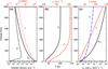 |
Fig. 1 Vertical profiles of Triton’s neutral atmosphere. (a) Number densities of the major species, N2 and N, and pressure, adopted from Krasnopolsky et al. (1993). (b) Neutral temperature and local sound speed, denoted T and cs, respectively. (c) Profiles of molecular (νm) and eddy (νe) kinematic viscosity, as well as the Brunt-Väisälä period (τb). |
2.3 Background atmosphere
Before solving for the linear wave solutions, the background atmospheric variables, including density, pressure, and temperature in the absence of waves, should be provided. The number densities of the two most abundant species, N2 and N, and pressure are shown in Fig. 1a, and the neutral temperature profile is presented in Fig. 1b. These background neutral atmospheric states are adopted from the recommended atmospheric model of Krasnopolsky et al. (1993). The local sound speed is calculated as  and also displayed in the panel b of Fig. 1, with values ranging from 130 to 200 m s−1. The Brunt-Väisälä frequency,
  , represents the characteristic oscillation frequency of an air parcel responding to external perturbations under the balance of gravity and buoyancy, where Γad = g/cp is the adiabatic lapse rate (e.g., Väisälä 1925; Brunt 1927; Nappo 2002; Wang et al. 2024), and
  . Correspondingly, the Brunt-Väisälä period is given by τb = 2π/ωb, with values ranging from 30 min to 145 min, as shown in Fig. 1c. Molecular viscosity, eddy viscosity, and thermal conduction are the main dissipation mechanisms for GWs in the upper atmosphere. The molecular kinetic viscosity and thermal diffusivity of Triton’s atmosphere are calculated from νm = μm/p and κm = λm/cp ρ, respectively, where μm and λm are the molecular dynamic viscosity and thermal conductivity. These quantities satisfy Pr = νm/Km and the thermal conductivity is expressed as λm = A Ts, with A = 2.6 erg cm−1 s−1 K−(1+s) and s = 1.3 for Triton’s N2-dominated, low-temperature atmosphere (Yelle et al. 1991). The Prandtl number is assumed to be Pr = 0.69. The eddy diffusion coefficient is expressed as
  (Herbert & Sandel 1991; Benne et al. 2022), where nN2 refers the number density of N2. In analogy with molecular viscosity, the eddy dynamic viscosity, μe, can be derived accordingly. The turbulent Prandtl number Prt = νe/Ke is assumed to be equal to 1, similar to that in Titan’s atmosphere (Huang et al. 2022, and references therein). The vertical profiles of νm and νe are shown in Fig. 1c, both increase approximately exponentially with altitude.
Near the surface, their values are about 2.51 × 10⁻⁸ km2 s−1 and 1.2 × 10⁻⁷ km2 s−1, while at an altitude of 1000 km in the upper atmosphere, they reach nearly 6.52 × 101 km2 s−1 and 2.84 × 10⁻³ km2 s−1, respectively.
3 Results
3.1 Input parameters
The wave model is time-independent with variations only in the vertical direction. By choosing different combinations of wave periods and horizontal wavelengths, we examined wave propagation over a wide range of temporal and spatial scales. Wave propagation was examined in the two-dimensional O-xz plane. In the horizontal direction, the waves were assumed to vary sinusoidally, corresponding to a plane-wave form. The model input parameters include the wave period (τ) and the horizontal wavelength, λx = 2π/kx. To examine the wave properties, we considered wave modes with different combinations of horizontal phase speeds (vp = ω/kx) and horizontal wavelengths. Previous studies suggest that the characteristic wind speeds in Triton’s atmosphere are on the order of 5 - 10 m s−1 (Ingersoll 1990; Yelle et al. 1991). Accordingly, the horizontal phase speeds are selected to be 5, 10, 15, and 20 m s−1 in this study. The horizontal wavelengths are taken to be 50, 100, and 200 km, which together span both short- and long-wavelength waves, as displayed in Table 2.
3.2 Wave propagations and damping properties
Fig. 2 displays the wave-induced relative temperature perturbation amplitudes, |T1/T0|, for three wave groups with horizontal wavelengths 50, 100, and 200 km. Each wave group consists of four wave modes with different horizontal phase speeds. The wave amplitude increases with altitude in the lower atmosphere. The conservation of wave energy leads to an inverse dependence of the amplitude on the square root of the background atmospheric density during the wave upward propagation. Due to the background atmospheric density decreases exponentially with altitude, the wave amplitude correspondingly increases with height. At higher altitudes, the molecular viscosity and thermal conduction become significant and progressively lead to the attenuation of waves. The wave amplitude attains a maximum at a certain altitude and then decays with increasing altitude.
The altitudes of maximum amplitude of the selected waves span roughly 50 - 300 km, as shown in Fig. 2. For a fixed horizontal wavelength, higher horizontal phase speeds correspond to higher wave frequencies, resulting in higher altitudes for the maximum wave amplitudes. For wave modes with shorter horizontal wavelengths, the maximum amplitudes are smaller than those of longer-wavelength modes. For a wavelength of 50 km, the maximum amplitude is less than 4%, as displayed in Fig. 2a. While for wavelengths of 100 km and 200 km, the maximum amplitudes reach approximately 7% and 9%, as illustrated in the panels b and c of Fig. 2, respectively. It is noted that for λx = 50 km and vp = 15 m s−1 and 20 m s−1, these two wave modes predominantly exhibit standing-wave behavior, undergoing reflection from a weakly evanescent region, as displayed in Fig. 2a. This occurs because their wave frequencies (corresponding to periods of approximately 56 and 42 min, respectively) are close to the local Brunt-Väisälä frequency.
The maximum amplitudes of the perturbed pressure and density are presented in Figs. 3a and 3b, respectively. As with temperature perturbations, higher horizontal phase speeds or longer horizontal wavelengths lead to larger maximum amplitudes. The maximum pressure perturbations range from approximately 0.1% to 1.8%, whereas the maximum density perturbations range from about 1% to 9%. These results indicate that the waves predominantly exhibit the characteristics of internal GWs, with density and temperature perturbations of comparable magnitude, while the compressional effects, indicated by the pressure perturbations, remain relatively small.
A representative wave mode with λx = 100 km and vp = 15 m s−1 is selected to provide a detailed illustration of wave propagation, and its density, temperature, and velocity perturbations are shown in Fig. 4. The left two panels, a and c, display the vertical distributions of density and temperature perturbations, as well as horizontal and vertical velocity perturbations, respectively. The right two panels, b and d, show the corresponding horizontal distributions.
As presented in Fig. 4a, the perturbed temperature and density exhibit an approximately antiphase relationship, which is characteristic of internal GWs. When a parcel of air is lifted to its maximum altitude, the local density perturbation reaches a maximum, while the parcel expands and cools, resulting in a minimum in the local temperature perturbation. Conversely, when the air parcel descends to its minimum altitude, the local density perturbation attains a minimum, and the parcel is compressed and heated, producing a maximum in the local temperature perturbation. This antiphase relationship can be quantitatively derived from the polarization relations. Under the incompressible approximation, the density and temperature perturbations can be simplified as  (Wang et al. 2024). This relation implies that the phase of the density perturbation leads the vertical velocity by π/2,
  , while the phase of the temperature perturbation lags the vertical velocity by π/2, φρ1 = φw1 + π/2. That is, the density perturbation is approximately 180° ahead of the temperature perturbation. However, as the waves propagate into the upper atmosphere and are dissipated by molecular viscosity and thermal conduction, the temperature perturbations no longer follow the density perturbations exactly, resulting in a phase shift between them. As shown in the three panels of Fig. 4b, the horizontal temperature and density perturbations exhibit different phase relations at altitudes of 100 km, 300 km, and 500 km. At 100 km, the waves behave essentially adiabatically, with a phase angle of 180° between temperature and density perturbations. As altitude increases, at 500 km, the temperature perturbations lag significantly behind the density perturbations, with a phase angle exceeding 180°.
The altitude profiles of the perturbed horizontal and vertical velocities, u1 and w1, are illustrated in Fig. 4c, and they exhibit a nearly synchronous phase relationship. Under the adiabatic, incompressible approximation, u1 and w1 satisfy u1 = (kz/kx) w1. As shown in Fig. 4d, at an altitude of 100 km, u1 and w1 are in phase. As the waves propagate to higher altitudes and are dissipated, the vertical velocity perturbation decreases, and w1 gradually lags behind u1.
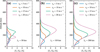 |
Fig. 2 Amplitudes of the wave temperature pertubation ratios. Panels a-c correspond to the waves with horizontal wavelengths (λx) of 50, 100, and 200 km, respectively. Each wavelength is associated with four different horizontal phase speeds (vp): 5, 10, 15, and 20 m s−1. |
Wave parameters and maximum perturbation amplitudes for different horizontal wavelengths and phase speeds.
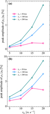 |
Fig. 3 Distributions of the peak amplitudes of (a) pressure perturbation ratios, p1/p0, and (b) density perturbation ratios, ρ1/ρ0. Horizontal wavelengths are 50, 100, and 200 km, and horizontal phase speeds are 5, 10, 15, and 20 m s−1. |
3.3 Wave-induced heating and cooling effects
As the waves are dissipated by molecular viscosity and thermal conduction in the upper atmosphere, the energy carried by the waves is released into the background atmosphere, affecting the redistribution of the thermal structure in the upper atmosphere.
The wave heating rate can be determined quantitatively from the following expression (Hickey et al. 2000; Schubert et al. 2003; Wang et al. 2020, 2024):
 (8)
(8)
where the terms in the right-hand side represent the sensible heating rate, the viscous heating rate, the work done per unit time by the wave-induced pressure gradient, and the work done per unit time by the second-order wave-induced Eulerian drift, respectively. Here Qtot is expressed in units of kelvin per Earth day (K day−1). The operator  in Eq. (8) denotes the wave-cycle time average of the product of two physical quantities, specifically computed as
  , where A and B are arbitrary complex functions, the subscript “*” denotes the complex conjugate, “Re” indicates the real part, and δφ is the phase difference between A and B. The corresponding heating energy flux is calculated by
  .
.
The wave heating rate and energy flux for the representative wave mode with λx = 100 km and vp = 15ms−1 are shown in Figs. 5a and 5b, respectively. Fig. 5a illustrates that Qpress and Qeuler correspond to reversible mechanical energy exchange terms, which exactly cancel in a non-dissipative atmosphere. When dissipation is present, this cancellation is incomplete, yielding a net heating or cooling effect (Schubert et al. 2003; Lian & Yelle 2019). The viscous heating rate provides a persistent contribution to the net heating. In the upper atmosphere, molecular viscosity becomes increasingly significant, causing waves to dissipate energy and momentum into the background atmosphere through viscous processes, thereby directly contributing to atmospheric heating. Qvis reach approximately 0.32 K day−1, occurring at altitude of approximately 273 km. The sensible heating rate, obtained from the negative divergence of the sensible heat flux,  , induces cooling in the upper atmosphere and heating in the lower atmosphere. In general, whether the sensible heat flux acts as a heating or cooling source is primarily governed by the phase difference between w1 and T1 as well as the wave amplitude (e.g., Schubert et al. 2003). The sensible heating rate reaches a maximum heating rate of approximately 0.62 K day−1 and a maximum cooling rate of 1.72 K day−1, occurring at altitudes of 229 km and 302 km, respectively. The total heating rate is dominated by the sensible heating component, reaching a maximum heating rate of approximately 0.78 K day−1 and a maximum cooling rate of about 1.54 K day−1. These correspond to volumetric heating and cooling rates of approximately 2.48 × 10⁻¹⁰ erg cm−3 s−1 and 0.96 × 10⁻¹⁰ erg cm−3 s−1, respectively, as listed in Table 3.
Correspondingly, the wave energy flux is shown in Fig. 5b. The total energy flux exhibits positive and negative values in the lower and upper regions, respectively, indicating that wave energy is transported upward in the lower atmosphere, where waves propagate in an approximately adiabatic environment. In the upper atmosphere, the wave energy flux is deposited into the background atmosphere as a result of wave dissipation induced by molecular viscosity and thermal conduction.
Figures 6a, 6b, and 6c present the altitude profiles of the total heating rate for wave groups with horizontal wavelengths of 50 km, 100 km, and 200 km, respectively. For a given horizontal wavelength, both the heating and cooling rates generally increase with increasing horizontal phase speed, and their peak values tend to occur at higher altitudes. An exception occurs for the wave mode with λx = 50 km and vp = 20 m s−1, whose period is very close to the local Brunt-Väisälä frequency, causing partial reflection from a weakly evanescent region. For all selected wave modes, the maximum heating rate occurs at lower altitudes, whereas the strongest cooling rate appears at higher altitudes. Although the magnitude of the maximum cooling rate is generally larger than that of the maximum heating rate, the corresponding volumetric heating rate exceeds the volumetric cooling rate, as listed in Table 3. This difference arises from the strong vertical decrease in the background atmospheric density. While large cooling rates occur in the upper atmosphere, the much lower background density there reduces the associated volumetric cooling rate, resulting in a maximum volumetric heating rate that is larger than the maximum volumetric cooling rate. For wave modes with a phase speed of 5 m s−1, the heating and cooling effects occur primarily below 150 km, whereas for higher phase-speed waves these effects extend to altitudes above 150 km.
 |
Fig. 4 Spatial distributions of (a, b) the density and temperature perturbation ratios (ρ1/ρ0) and (T1/T0), as well as (c, d) the horizontal (u1) and vertical velocity perturbations (w1) for the selected wave mode. Panels a and c present the vertical profiles of the perturbations. Panels b and d show the horizontal distributions at selected altitudes of 100, 300, and 500 km. The horizontal wavelength (λx), the horizontal phase speed (vp), and the period (τ) of the selected wave mode are 100 km, 15 m s−1, and 1.85 h, respectively. |
3.4 Wave-driven thermal variations
The wave heating or cooling in the upper atmosphere ultimately contributes to the thermal structure of the background atmosphere. To estimate the thermospheric temperature response associated with the calculated wave heating and cooling rates, we solved the following steady-state energy balance equation:
 (9)
(9)
where λm = A Ts denotes the thermal conductivity; A = 2.6 erg cm−1 s−1 K−(1+s) and s = 1.3 for Triton’s atmosphere (Yelle et al. 1991).
Equation (9) provides a simplified steady-state estimate of the thermal response of the background atmosphere to wave-induced heating and cooling. It should be noted that this formulation does not explicitly account for the temporal evolution of the temperature profile or the potential two-way feedback between the evolving thermal structure and GW propagation. In reality, wave dissipation can modify the background temperature structure, which in turn can influence subsequent wave propagation and dissipation characteristics. A fully self-consistent treatment would therefore require solving the time-dependent energy equation together with the wave dynamics, allowing for the bidirectional coupling between the evolving temperature field and wave-induced heating. Such a coupled framework is beyond the scope of the present study. Instead, the present calculation aims to provide a first-order estimate of the magnitude of the thermospheric temperature variations associated with the simulated wave heating and cooling rates, similar to approaches adopted in previous studies of wave-driven thermospheric heating (e.g., Hickey et al. 2000; Schubert et al. 2003; Wang et al. 2020, 2025, 2026).
This work focuses on the impact of wave-induced heating on the thermal structure of the Triton’s thermosphere. The integration domain and boundary conditions are consistent with Stevens et al. (1992). The boundary conditions are specified as T = T0 at the tropopause (8 km) and zero net heat flux at the upper boundary, i.e., ∂T/∂z = 0. Therefore, the solution to Eq. (9) is:
![Mathematical equation: T(z) = \left[T_{0}^{s+1}(z)+\frac{s+1}{A}\int_{z_{0}}^{z}F_{tot}(z) \, dz\right]^{\frac{1}{s+1}}](/articles/aa/full_html/2026/04/aa58830-25/aa58830-25-eq26.png) (10)
(10)
where z0 denotes the reference altitude and equals to 8 km.
Equation (10) describes the temperature associated with the wave heating/cooling effects. The difference between the wave-driven temperature and the background temperature is given by δT = T - T0, which is illustrated in Figs. 6d-f for the selected wave groups. The maximum temperature difference occurs at the altitude of peak wave heating rates. The selected wave modes contribute to net heating in the upper atmosphere. For shortwavelength waves, the total temperature increase is less than 20 K. For waves with a horizontal wavelength of 50 km, phase speeds of 5, 10, 15, and 20 m s−1 produce temperature increases near the exobase of about 4, 6, 11, and 2 K, respectively, as also listed in Table 3. Note that the wave mode with λx = 50 km and vp = 20 m s−1 has a relatively weak effect on the upper atmospheric thermal structure due to its reflection in the lower region. For long-wavelength wave modes, the temperature near the exobase can enhance several tens of kelvins. Specifically, the temperature increases are approximately 5, 10, 25, and 43 K for the horizontal wavelength of 100 km, with the horizontal phase speeds of 5, 10, 15, and 20 m s−1, respectively. For the wave modes with λx = 200 km, the corresponding temperature increase are about 5, 16, 40, and 71 K, respectively.
Wave-induced heating and cooling rates and the resulting exospheric temperature response.
4 Discussions and concluding remarks
Early studies suggest that magnetospheric electron transport, energy deposition, and solar radiations play an important role in the variations in Triton’s upper atmospheric thermal structure (e.g., Lyons et al. 1992; Sittler & Hartle 1996; Benne et al. 2024). It is well recognized that GWs play a fundamental role in transporting and redistributing momentum and energy in planetary atmospheres, thereby contributing to the thermal structure and energy balance of the upper atmosphere (e.g., Hines 1960; Yeh & Liu 1974; Lindzen 1981; Walterscheid 1981; Holton 1983; Fritts 1984; Matcheva & Strobel 1999; Fritts & Alexander 2003; Yiğit & Medvedev 2009; Hickey et al. 2011; Wang et al. 2020, 2024, 2025, 2026). Such waves have not been directly observed in Triton’s atmosphere, but may be generated by potential wavegeneration mechanisms, including geyser-like plumes near the surface, energetic particle deposition, and solar radiation (e.g., Smith et al. 1989; Soderblom et al. 1990; Ingersoll 1990; Lyons et al. 1992; Sittler & Hartle 1996). In this study, we used a linear full-wave model to investigate the heating and cooling effects on Triton’s upper atmosphere. Based on the measured characteristics of plumes, we used a Gaussian source in the model to simulate waves excited by geyser-like plumes. By selecting different wavelengths and phase speeds, we investigated the impact of wave modes with varying temporal and spatial scales on the background atmosphere. Our results demonstrate that GWs play a critical role in driving variations in the thermal structure. Our main findings are summarized as follows.
First, the waves propagate adiabatically in the lower atmosphere, where the density and temperature perturbations remain antiphased and the horizontal and vertical velocities are inphase. The wave amplitudes increase with height. However, molecular viscosity and thermal conduction become dominant when the waves propagate into the upper region, contributing to wave dissipation. In the dissipative region, the temperature perturbation lags the density perturbation by over 180° and a phase shift occurs, with the vertical velocity lagging the horizontal velocity. For wave modes with short wavelengths and low-phase speeds, their peak amplitude occurs below 200 km. In contrast, for modes with long wavelengths and high-phase speeds, the peak can occur at altitudes of up to 300 km. The peak perturbed temperature and density ratio is less than 5% for wave modes with a horizontal wavelength of 50 km, but it can reach 7% and 9% for those with horizontal wavelengths of 100 km and 200 km, respectively. The pressure perturbation ratios are less than 2% for all selected wave modes.
The dissipation of waves by molecular viscosity and thermal conduction modifies the thermal structure of the background atmosphere. Our results indicate that the wave-induced thermal effect is driven primarily by the sensible heating effect. Specifically, waves heat the lower atmosphere and cool the upper atmosphere. This finding is consistent with the role of waves in the atmospheres of other planets and satellites. (e.g., Hickey et al. 2000; Schubert et al. 2003; Hickey et al. 2011; Wang et al. 2020, 2024). For wave modes with low-phase speeds, the peaks of both heating and cooling rates occur below 200 km in altitude. In contrast, for modes with high-phase speeds, the heating or cooling effects can extend up to the 400 km altitude region. The magnitudes of the wave heating and cooling rates in the Triton’s atmosphere can reach the order of 10−10 erg cm−3 s−1, with the heating rate exceeding the cooling rate, and the associated wave energy flux reaches 10−3 erg cm−2 s−1. These results imply that the wave-induced heating is comparable in magnitude to the heating rates associated with magnetospheric electron precipitation and solar EUV radiation reported in previous studies (Stevens et al. 1992; Krasnopolsky et al. 1993; Strobel & Zhu 2017). The wave-induced temperature was calculated from the energy balance equation. The results indicate that all the selected waves can heat the whole atmosphere. The temperature at the exobase increases by approximately 2-11 K for short-wavelength waves (λx = 50 km), whereas larger increases of about 5-43 K and 5-71 K are obtained for wave modes with λx = 100 km and λx = 200 km, respectively. For a given horizontal wavelength, the magnitude of the temperature increases with the horizontal phase speed. Specifically, wave modes with v p = 5 m s−1 produce temperature rises of only a few kelvins, whereas those with vp = 20 m s−1 can induce heating of approximately 40 K and 70 K for λx = 100 km and λx = 200 km, respectively. This result is consistent with the calculations of Stevens et al. (1992), in which an energy balance approach was used to evaluate the thermal response to solar and equatorial magnetospheric power inputs. In that study, the temperature at the exobase reached 181 K, corresponding to an increase of about 85 K. These results indicate that the heating effects of GWs are comparable to those of solar EUV radiation and magnetospheric particle precipitation, and, thus, play an important role in the thermal balance of Triton’s upper atmosphere.
This study provides a comprehensive comparison of wave behavior in the atmospheres of different planets and satellites. For Titan, which has a N2-dominated atmosphere similar to that of Triton, wave heating rates are also on the order of 10−10 erg cm−3 s−1. However, only waves with horizontal phase speeds exceeding 69 m s−1 are capable of producing a temperature increase of about 7 K at Titan’s exobase. This weaker heating mainly results from Titan’s much denser atmosphere, which causes stronger wave damping. In addition, Titan’s exobase is located at a higher altitude of about 1500 km, compared with about 850 km for Triton, further contributing to the different heating efficiencies in the two atmospheres. Although haze layering induced by GWs has been observed in Pluto’s atmosphere (Gladstone et al. 2016; Cheng et al. 2017), which is similar to that of Triton, the heating effects of these waves in Pluto’s atmosphere are still not well understood. This study provides a useful reference and suggests that GWs also contribute to heating in Pluto’s upper atmosphere.
This study adopted a linear wave model and primarily focused on the thermodynamic heating and cooling effects associated with wave dissipation in Triton’s upper atmosphere. In addition to direct thermal effects, GWs are well known to transport momentum during their vertical propagation and to deposit this momentum when dissipating, thereby modifying the background circulation through wave mean-flow interactions (e.g., Lindzen 1981; Holton 1983; Fritts 1984). The resulting momentum deposition can drive secondary circulations that further influence the thermal structure of the atmosphere through adiabatic heating and cooling and large-scale energy redistribution (e.g., Yiğit et al. 2008; Medvedev & Yiğit 2019). These coupled dynamical thermal processes are widely recognized as an important pathway through which GWs affect the structure and energetics of planetary atmospheres.
In the present work, however, we restricted our analysis to the direct wave-induced heating and cooling rates diagnosed from the linear wave solution. Nonlinear processes and the associated dynamical feedbacks, including wave breaking, saturation, ducting, and momentum-driven secondary circulation, were not explicitly modeled. For example, the linear results indicate that the wave mode with a horizontal wavelength of 50 km and a phase speed of 20 m s−1 is reflected below an altitude of about 100 km and may form a standing-wave structure. In a realistic atmosphere, the presence of background winds could further modify the wave propagation and lead to wave mean-flow interactions. A fully self-consistent treatment of these nonlinear processes would require a more comprehensive dynamical framework and is therefore left for future studies.
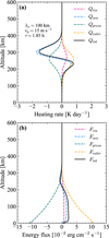 |
Fig. 5 (a) Heating rate profiles and (b) wave energy flux profiles for the selected wave mode. The wave parameters are the same as those in Fig. 4. The heating rates (in K day−1) include contributions from viscous heating (Qvis), the negative divergence of the sensible heat flux (Qsen), the wave-induced pressure gradient (Qpress), the second-order Eulerian drift (Qeuler), and the total heating rate (Qtot). The corresponding energy flux components (in erg cm−2 s−1) are labeled using the same notation. |
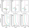 |
Fig. 6 Total heating rate and wave-driven temperature perturbation profiles for the selected wave modes. Panels a-c show the total heating rate, Qtot. Panels d-f display the temperature difference between the wave-induced temperature and the mean-state temperature, δT. From left to right, the horizontal wavelengths, λx, are 50, 100, and 200 km. For each wavelength, the horizontal phase speeds, vp, are 5, 10, 15, and 20 m s−1. |
Acknowledgements
This work is supported by the National Natural Science Foundation of China (Grants 12522308, 42241114, 42422406, 42174185, 42475134, 42274218) and the Science and Technology Development Fund, Macau SAR (File no. 0042/2024/RIA1, 0008/2024/AKP, and 002/2024/SKL).
References
- Barrow, D., & Matcheva, K. I. 2011, Icarus, 211, 609 [NASA ADS] [CrossRef] [Google Scholar]
- Barrow, D. J., & Matcheva, K. I. 2013, Icarus, 224, 32 [NASA ADS] [CrossRef] [Google Scholar]
- Benne, B., Dobrijevic, M., Cavalié, T., Loison, J.-C., & Hickson, K. M. 2022, A&A, 667, A169 [NASA ADS] [CrossRef] [EDP Sciences] [Google Scholar]
- Benne, B., Benmahi, B., Dobrijevic, M., et al. 2024, A&A, 686, A22 [NASA ADS] [CrossRef] [EDP Sciences] [Google Scholar]
- Broadfoot, A. L., Atreya, S. K., Bertaux, J. L., et al. 1989, Science, 246, 1459 [NASA ADS] [CrossRef] [Google Scholar]
- Brown, Z. L., Medvedev, A. S., Starichenko, E. D., Koskinen, T. T., & Müller-Wodarg, I. C. F. 2022, Geophys. Res. Lett., 49, e97219 [NASA ADS] [Google Scholar]
- Brunt, D. 1927, Quart. J. Roy. Metor. Soc., 53, 30 [NASA ADS] [CrossRef] [Google Scholar]
- Cheng, A. F., Summers, M. E., Gladstone, G. R., et al. 2017, Icarus, 290, 112 [CrossRef] [Google Scholar]
- Cruikshank, D. P., Matthews, M. S., & Schumann, A. M., eds. 1995, Neptune and Triton [Google Scholar]
- Cui, J., Lian, Y., & Müller-Wodarg, I. C. F. 2013, Geophys. Res. Lett., 40, 43 [NASA ADS] [CrossRef] [Google Scholar]
- Cui, J., Yelle, R. V., Li, T., Snowden, D. S., & Müller-Wodarg, I. C. F. 2014, J. Geophys. Res.(Space Phys.), 119, 490 [NASA ADS] [CrossRef] [Google Scholar]
- French, R. G., & Gierasch, P. J. 1974, J. Atmos. Sci., 31, 1707 [Google Scholar]
- Fritts, D. C. 1984, Rev. Geophys. Space Phys., 22, 275 [CrossRef] [Google Scholar]
- Fritts, D. C., & Alexander, M. J. 2003, Rev. Geophys., 41, 1003 [NASA ADS] [CrossRef] [Google Scholar]
- Gladstone, G. R., Stern, S. A., Ennico, K., et al. 2016, Science, 351, aad8866 [NASA ADS] [CrossRef] [Google Scholar]
- Gu, H., Cui, J., Niu, D.-D., et al. 2021, A&A, 650, A130 [NASA ADS] [CrossRef] [EDP Sciences] [Google Scholar]
- Gu, H., Cui, J., Wang, X., et al. 2024, J. Geophys. Res.(Space Phys.), 129, e2023JA032154 [Google Scholar]
- Hansen, C. J., McEwen, A. S., Ingersoll, A. P., & Terrile, R. J. 1990, Science, 250, 421 [NASA ADS] [CrossRef] [Google Scholar]
- Hansen, C. J., Castillo-Rogez, J., Grundy, W., et al. 2021, PSJ, 2, 137 [Google Scholar]
- Herbert, F., & Sandel, B. R. 1991, J. Geophys. Res., 96, 19241 [NASA ADS] [CrossRef] [Google Scholar]
- Hickey, M. P., Taylor, M. J., Gardner, C. S., & Gibbons, C. R. 1998, J. Geophys. Res., 103, 6439 [Google Scholar]
- Hickey, M. P., Walterscheid, R. L., & Schubert, G. 2000, Icarus, 148, 266 [NASA ADS] [CrossRef] [Google Scholar]
- Hickey, M. P., Walterscheid, R. L., & Schubert, G. 2011, J. Geophys. Res.(Space Phys.), 116, A12326 [Google Scholar]
- Hines, C. O. 1960, Can. J. Phys., 38, 1441 [NASA ADS] [CrossRef] [Google Scholar]
- Holton, J. R. 1983, J. Atmos. Sci., 40, 2497 [Google Scholar]
- Huang, J., Wu, Z., Cui, J., et al. 2022, J. Geophys. Res.(Planets), 127, e07310 [NASA ADS] [Google Scholar]
- Huang, X., Gu, H., & Cui, J. 2025, A&A, 702, A5 [NASA ADS] [CrossRef] [EDP Sciences] [Google Scholar]
- Ingersoll, A. P. 1990, Nature, 344, 315 [NASA ADS] [CrossRef] [Google Scholar]
- Krasnopolsky, V. A., Sandel, B. R., Herbert, F., & Vervack, R. J. 1993, J. Geophys. Res., 98, 3065 [NASA ADS] [CrossRef] [Google Scholar]
- Lian, Y., & Yelle, R. V. 2019, Icarus, 329, 222 [NASA ADS] [CrossRef] [Google Scholar]
- Lindzen, R. S. 1981, J. Geophys. Res., 86, 9707 [NASA ADS] [CrossRef] [Google Scholar]
- Lyons, J. R., Yung, Y. L., & Allen, M. 1992, Science, 256, 204 [NASA ADS] [CrossRef] [Google Scholar]
- Matcheva, K. I., & Barrow, D. J. 2012, Icarus, 221, 525 [NASA ADS] [CrossRef] [Google Scholar]
- Matcheva, K. I., & Strobel, D. F. 1999, Icarus, 140, 328 [NASA ADS] [CrossRef] [Google Scholar]
- Matcheva, K. I., Strobel, D. F., & Flasar, F. M. 2001, Icarus, 152, 347 [NASA ADS] [CrossRef] [Google Scholar]
- Medvedev, A. S., & Yiğit, E. 2012, Geophys. Res. Lett., 39, L05201 [NASA ADS] [CrossRef] [Google Scholar]
- Medvedev, A. S., & Yiğit, E. 2019, Atmosphere, 10, 531 [NASA ADS] [CrossRef] [Google Scholar]
- Medvedev, A. S., Klaassen, G. P., & Yiğit, E. 2023, J. Geophys. Res.(Space Phys.), 128, e2022JA031152 [NASA ADS] [CrossRef] [Google Scholar]
- Müller-Wodarg, I. C. F., Yelle, R. V., Borggren, N., & Waite, J. H. 2006, J. Geophys. Res. (Space Phys.), 111, A12315 [Google Scholar]
- Müller-Wodarg, I. C. F., Koskinen, T. T., Moore, L., et al. 2019, Geophys. Res. Lett., 46, 2372 [Google Scholar]
- Nappo, C. J. 2002, An Introduction to Atmospheric Gravity Waves, 85 [Google Scholar]
- Navarro, T., & Schubert, G. 2024, Geophys. Res. Lett., 51, e2023GL104922 [Google Scholar]
- Schubert, G., Hickey, M. P., & Walterscheid, R. L. 2003, Icarus, 163, 398 [NASA ADS] [CrossRef] [Google Scholar]
- Sittler, E. C., & Hartle, R. E. 1996, J. Geophys. Res., 101, 10863 [Google Scholar]
- Smith, B. A., Soderblom, L. A., Banfield, D., et al. 1989, Science, 246, 1422 [NASA ADS] [CrossRef] [Google Scholar]
- Soderblom, L. A., Kieffer, S. W., Becker, T. L., et al. 1990, Science, 250, 410 [Google Scholar]
- Stevens, M. H., Strobel, D. F., Summers, M. E., & Yelle, R. V. 1992, Geophys. Res. Lett., 19, 669 [NASA ADS] [CrossRef] [Google Scholar]
- Strobel, D. F., & Zhu, X. 2017, Icarus, 291, 55 [NASA ADS] [CrossRef] [Google Scholar]
- Tripathi, K. R., Choudhary, R. K., Jose, J. S., Ambili, K. M., & Imamura, T. 2023, Geophys. Res. Lett., 50, e2022GL101793 [Google Scholar]
- Väisälä, V. 1925, Soc. Sci. Fennica, Commentationes Phys.-Math. II, 19, 37 [Google Scholar]
- Walterscheid, R. L. 1981, Geophys. Res. Lett., 8, 1235 [Google Scholar]
- Walterscheid, R. L., Hickey, M. P., & Schubert, G. 2013, J. Geophys. Res.(Planets), 118, 2413 [Google Scholar]
- Wang, X., Lian, Y., Cui, J., et al. 2020, J. Geophys. Res.(Planets), 125, e06163 [NASA ADS] [Google Scholar]
- Wang, X., Xu, X., Cui, J., et al. 2023, MNRAS, 518, 4310 [Google Scholar]
- Wang, X., Xu, X., Cui, J., et al. 2024, A&A, 688, A24 [NASA ADS] [CrossRef] [EDP Sciences] [Google Scholar]
- Wang, X., Xu, X., Cui, J., et al. 2025, AJ, 169, 108 [Google Scholar]
- Wang, X., Cui, J., He, Z., et al. 2026, ApJ, 998, 265 [Google Scholar]
- Yeh, K. C., & Liu, C. H. 1974, Rev. Geophys. Space Phys., 12, 193 [CrossRef] [Google Scholar]
- Yelle, R. V., Lunine, J. I., & Hunten, D. M. 1991, Icarus, 89, 347 [NASA ADS] [CrossRef] [Google Scholar]
- Yiğit, E., & Medvedev, A. S. 2009, Geophys. Res. Lett., 36, L14807 [Google Scholar]
- Yiğit, E., & Medvedev, A. S. 2012, Geophys. Res. Lett., 39, L21101 [Google Scholar]
- Yiğit, E., & Medvedev, A. S. 2015, Adv. Space Res., 55, 983 [CrossRef] [Google Scholar]
- Yiğit, E., & Medvedev, A. S. 2017, J. Geophys. Res.(Space Phys.), 122, 4846 [CrossRef] [Google Scholar]
- Yiğit, E., Aylward, A. D., & Medvedev, A. S. 2008, J. Geophys. Res.(Atmos.), 113, D19106 [Google Scholar]
- Yiğit, E., Medvedev, A. S., Aylward, A. D., et al. 2012, J. Atmos. Solar-Terr. Phys., 90, 104 [Google Scholar]
- Yiğit, E., Medvedev, A. S., England, S. L., & Immel, T. J. 2014, J. Geophys. Res.(Space Phys.), 119, 357 [Google Scholar]
- Yiğit, E., Medvedev, A. S., & Hartogh, P. 2015, Geophys. Res. Lett., 42, 4294 [CrossRef] [Google Scholar]
- Yiğit, E., Medvedev, A. S., & Hartogh, P. 2018, Ann. Geophys., 36, 1631 [CrossRef] [Google Scholar]
- Yiğit, E., Medvedev, A. S., Benna, M., & Jakosky, B. M. 2021, Geophys. Res. Lett., 48, e92095 [Google Scholar]
- Young, L. A., Yelle, R. V., Young, R., Seiff, A., & Kirk, D. B. 1997, Science, 276, 108 [NASA ADS] [CrossRef] [Google Scholar]
- Young, L. A., Yelle, R. V., Young, R., Seiff, A., & Kirk, D. B. 2005, Icarus, 173, 185 [NASA ADS] [CrossRef] [Google Scholar]
All Tables
Adopted planetary, thermodynamic, and wave-source parameters for Triton used in this study.
Wave parameters and maximum perturbation amplitudes for different horizontal wavelengths and phase speeds.
Wave-induced heating and cooling rates and the resulting exospheric temperature response.
All Figures
|
Fig. 1 Vertical profiles of Triton’s neutral atmosphere. (a) Number densities of the major species, N2 and N, and pressure, adopted from Krasnopolsky et al. (1993). (b) Neutral temperature and local sound speed, denoted T and cs, respectively. (c) Profiles of molecular (νm) and eddy (νe) kinematic viscosity, as well as the Brunt-Väisälä period (τb). |
| In the text | |
|
Fig. 2 Amplitudes of the wave temperature pertubation ratios. Panels a-c correspond to the waves with horizontal wavelengths (λx) of 50, 100, and 200 km, respectively. Each wavelength is associated with four different horizontal phase speeds (vp): 5, 10, 15, and 20 m s−1. |
| In the text | |
|
Fig. 3 Distributions of the peak amplitudes of (a) pressure perturbation ratios, p1/p0, and (b) density perturbation ratios, ρ1/ρ0. Horizontal wavelengths are 50, 100, and 200 km, and horizontal phase speeds are 5, 10, 15, and 20 m s−1. |
| In the text | |
|
Fig. 4 Spatial distributions of (a, b) the density and temperature perturbation ratios (ρ1/ρ0) and (T1/T0), as well as (c, d) the horizontal (u1) and vertical velocity perturbations (w1) for the selected wave mode. Panels a and c present the vertical profiles of the perturbations. Panels b and d show the horizontal distributions at selected altitudes of 100, 300, and 500 km. The horizontal wavelength (λx), the horizontal phase speed (vp), and the period (τ) of the selected wave mode are 100 km, 15 m s−1, and 1.85 h, respectively. |
| In the text | |
|
Fig. 5 (a) Heating rate profiles and (b) wave energy flux profiles for the selected wave mode. The wave parameters are the same as those in Fig. 4. The heating rates (in K day−1) include contributions from viscous heating (Qvis), the negative divergence of the sensible heat flux (Qsen), the wave-induced pressure gradient (Qpress), the second-order Eulerian drift (Qeuler), and the total heating rate (Qtot). The corresponding energy flux components (in erg cm−2 s−1) are labeled using the same notation. |
| In the text | |
|
Fig. 6 Total heating rate and wave-driven temperature perturbation profiles for the selected wave modes. Panels a-c show the total heating rate, Qtot. Panels d-f display the temperature difference between the wave-induced temperature and the mean-state temperature, δT. From left to right, the horizontal wavelengths, λx, are 50, 100, and 200 km. For each wavelength, the horizontal phase speeds, vp, are 5, 10, 15, and 20 m s−1. |
| In the text | |
Current usage metrics show cumulative count of Article Views (full-text article views including HTML views, PDF and ePub downloads, according to the available data) and Abstracts Views on Vision4Press platform.
Data correspond to usage on the plateform after 2015. The current usage metrics is available 48-96 hours after online publication and is updated daily on week days.
Initial download of the metrics may take a while.