| Issue |
A&A
Volume 708, April 2026
|
|
|---|---|---|
| Article Number | A328 | |
| Number of page(s) | 7 | |
| Section | Astrophysical processes | |
| DOI | https://doi.org/10.1051/0004-6361/202558077 | |
| Published online | 21 April 2026 | |
Multi-wavelength emission modelling of PSR J0437–4715
1
Université de Strasbourg, CNRS, Observatoire Astronomique de Strasbourg, UMR 7550, F-67000 Strasbourg, France
2
IRAP, CNRS, 9 Avenue du Colonel Roche, BP 44346, F-31028 Toulouse Cedex 4, France
3
LPC2E, OSUC, Univ Orléans, CNRS, CNES, Observatoire de Paris, F-45071 Orléans, France
4
ORN, Observatoire de Paris, Université PSL, Univ. Orléans, CNRS, 18330 Nançay, France
★ Corresponding author: This email address is being protected from spambots. You need JavaScript enabled to view it.
Received:
12
November
2025
Accepted:
11
March
2026
Abstract
Context. The diversity of pulsar light curves and radio polarisation properties originates in the structure of the magnetic field close to the stellar surface. For millisecond pulsars, this complexity is particularly puzzling. Fortunately, some means exist to uncover the magnetic field topology that indeed impacts the emission within the magnetosphere but also on the surface through its hot spot thermal radiation.
Aims. We aim at deducing a plausible magnetic field geometry for the millisecond pulsar J0437−4715 by using combined information from the soft X-ray hot spot geometry deduced from NICER observations by pulse profile modelling and from radio and γ-ray pulse profile fitting. We also check the consistency between the obtained geometry and the radio polarisation data.
Methods. Our γ-ray light-curve shapes rely on the striped wind model, whereas the radio polarisation fits rely on the rotating vector model. The magnetosphere structure is obtained from dipolar force-free magnetosphere simulations.
Results. We demonstrate that a slightly off-centred dipole augmented by a small-scale dipole located on one polar cap explains simultaneously the shape of the hot spot and the radio and γ-ray data with a magnetic obliquity of α ≈ (42 ± 5)° and a line-of-sight inclination angle of ζ ≈ (136 ± 5)°.
Conclusions. Our simple dipole model reproduces all the radio and γ-ray characteristics of PSR J0437−4715, including its radio polarisation data. It shows that the radio emission could be produced in regions where the magnetic field is mainly of dipolar nature.
Key words: magnetic fields / methods: numerical / pulsars: general / stars: rotation / pulsars: individual: PSR J0437–4715
© The Authors 2026
 Open Access article, published by EDP Sciences, under the terms of the Creative Commons Attribution License (https://creativecommons.org/licenses/by/4.0), which permits unrestricted use, distribution, and reproduction in any medium, provided the original work is properly cited.
This article is published in open access under the Subscribe to Open model. This email address is being protected from spambots. You need JavaScript enabled to view it. to support open access publication.
1. Introduction
Millisecond pulsars (MSPs) are fast rotating neutron stars that experienced spin-up during their accretion phase in a binary system. This spin-up mechanism leads to rotational periods in MSPs as fast as several milliseconds. These stars are old pulsars, aged billions of years, with weak surface magnetic field strengths of the order of 103 T–105 T (107 G–109 G). Deciphering their magnetic field structure is a difficult task due to the small size of the neutron star magnetosphere (characterised by the light cylinder radius defined by rL = c/Ω where c is the speed of light and Ω the stellar angular velocity) and due to the strong impact of near surface multipolar or small-scale magnetic fields. Nevertheless, attempts have been made to extract this field geometry by combining radio, soft X-ray, and γ-ray emission in several MSPs observed with the Neutron star Interior Composition ExploreR (NICER), such as PSR J0030+0451 (Pétri et al. 2023) or PSR J0740+6620 (Pétri et al. 2025). Determining the shape of the hot spots located at the neutron star surface could offer valuable insight into the near surface magnetic field configuration and serve as an input for global magnetospheric simulations. This task was undertaken by using NICER data to analyse four MSPs: PSR J0030+0451 (Riley et al. 2019; Miller et al. 2019; Vinciguerra et al. 2024), PSR J0740+6620 (Salmi et al. 2022; Miller et al. 2021; Dittmann et al. 2024), and PSR J1231−1411 (Salmi et al. 2024) (see also Bogdanov et al. 2019 for earlier results). More recently Choudhury et al. (2024) analysed PSR J0437−4715 and found two non-antipodal hot spots, whereas Mauviard et al. (2025) studied PSR J0614−3329 and found two hot spots, one close to the pole and the other close to the equator. PSR J0437−4715 is the nearest and brightest MSP known so far with soft X-ray emission, and it is the target of interest in the present study.
The discovery of the X-ray emission of PSR J0437−4715 dates back to observations with the ROntgenSATellit (ROSAT) telescope (Becker & Trümper 1993). The thermal nature of this emission (Pavlov & Zavlin 1997; Zavlin & Pavlov 1998) was used for detailed modelling of its spectrum and of the pulsed profile resulting from the neutron star rotation (Zavlin et al. 2002; Zavlin 2006). Bogdanov (2013) performed the first phase-resolved spectroscopic study of this pulsar and provided some constraints on its compactness. Later, a broad-band X-ray analysis demonstrated the presence of three thermal components (the warm surface and two hot spots), characterised the non-thermal spectral component, and showed pulsations up to ∼15 keV with data from the Nuclear Spectroscopic Telescope Array (NuSTAR; Guillot et al. 2016). The warm surface, at Teff ∼ 2 × 10⁵ K, was further studied by combining the X-ray data and far-ultraviolet observations with the Hubble Space Telescope (González-Caniulef et al. 2019). In the radio, this pulsar has been known since the 1990s (Johnston et al. 1993), and its polarised radio emission was studied in Navarro et al. (1997). A single radio pulse analysis was performed in Osłowski et al. (2014).
From a theoretical point of view, several groups have tackled the problem of connecting the hot spot geometry to the external magnetic field computed from the magnetosphere, including, for instance, a quadrupole component, as in Lockhart et al. (2019). Multipolar components were also suspected in the PSR J0030+4051 (Kalapotharakos et al. 2021). Huang & Chen (2025), based on a force-free magnetosphere of an off-centred magnetic dipole, deduced the polar cap temperature distribution and predicted the observed X-ray light curves, see also Huang (2026) for fully analytical expressions for surface return currents. Chen et al. (2020) did a similar analysis for PSR J0030+0451 using a dipole and quadrupole configuration. Dyks (2019) explained the complexity of the radio polarisation data in terms of a coherent superposition of orthogonal modes. Finally, Sur et al. (2024) performed force-free simulations with multipoles and applied it to MSPs. One hot spot of PSR J0437−4715 as found by Choudhury et al. (2024) shows an annular shape that is interpreted as the presence of a quadrudipole field, i.e. a combination of a dipole and a quadrupole (Gralla et al. 2017). More quantitatively, Carrasco et al. (2023) performed general-relativistic force-free (GRFFE) simulations of neutron star magnetospheres to model the soft X-ray pulse profile of several NICER pulsars, including PSR J0437−4715. Their work is based on the electric current circulating within the magnetosphere in the force-free regime, leading to non-standard emission regions (different from the almost circular polar cap regions).
Notably, PSR J0437−4715 is the fourth pulsar with pulse-profile modelling analyses published by the NICER team. It is detected in radio and γ-rays with good quality radio polarisation data, as summarised in Sect. 2. Based on these multi-wavelength observations, we inferred the magnetic field geometry of the radio emission site, as explained in Sect. 3. Our conclusions are presented in Sect. 4.
2. PSR J0437–4715 multi-wavelength observations
2.1. Observational facts
The PSR J0437−4715 is an MSP spinning at a period of P = 5.75 ms and orbiting in a binary system with a white dwarf companion at a period of Porb = 5.74 day. Its orbital inclination angle, derived from Shapiro delay measurements, has been accurately determined to be i = 137.506° ±0.016° (Reardon et al. 2024), and its mass was found to be M = 1.418 M⊙ ± 0.044 M⊙. Pulse profile modelling performed by Choudhury et al. (2024) tends to a radius of 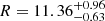 km. This leads to a ratio between the neutron star radius and its light-cylinder radius of a = R/rL ≈ 0.0414, where rL = c P/2π ≈ 274 km, and a polar cap angular size of
  .
.
2.2. Radio and γ-rays observations
The PSR J0437−4715 was among the first radio MSPs detected in γ-rays with Fermi/LAT (Abdo et al. 2009). Updated γ-ray emission properties have been published more recently in the third γ-ray pulsar catalogue (3PC; Smith et al. 2023). Its multi-wavelength pulse profile, taken from 3PC for the radio and γ-ray part and from NICER for the X-ray part (see the next subsection), is shown in Fig. 1. The profile shows a single wide radio pulse spanning almost the full period, with a duty cycle of 80%. The single γ-ray peak is separated from this radio peak by approximately 0.4 in phase, whereas the soft X-ray peak is almost aligned with the radio pulse peak.
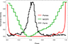 |
Fig. 1. Multi-wavelength pulse profile of PSR J0437−4715 as observed in the radio by Parkes at 1.4 GHz (red line), in soft X-rays by NICER (0.3−3.0 keV, green line), and in γ-rays by Fermi/LAT (black line). Note that the zero line of the NICER data is arbitrary since, technically, the pulsed emission lies on top of an un-pulsed pulsar emission plus background emission (all origins combined). We note that this is also true for the radio data, for which the profile baseline has been subtracted to lie at zero. |
Good radio polarisation data have also been published by Dai et al. (2015) and are available on the European Pulsar Network (EPN) database. The polarisation position angle (PPA) is complex and does not reflect the rotating vector model (RVM) expectation, probably due to multipolar components or to emission height variation, twisted magnetic field lines, and orthogonal polarisation modes (OPMs).
2.3. NICER data
We generated the NICER X-ray pulse profile of PSR J0437−4715 following the standard data reduction procedure1 on the X-ray Timing Instrument (XTI) observations from 2017-07-06:T14:34:12 to 2023-05-21:T22:22:27 (ObsIDs: 0060010101-6060010721). Because of an optical light leak2 resulting from NICER thermal film damage on 22 May 2023, observations since this date have been ignored. In addition, a handful of observations presented time stamp anomalies on the detectors of the Measurement Power Unit 1 because of a single-event upset3 affecting the XTI (affected ObsIDs: 2060010407-2060010412) when NICER was passing through the South Atlantic Anomaly. Those events have been excluded as well.
The remaining data have been calibrated and filtered with the nicerl2 tool from NICERDAS v13, provided with HEASOFT v6.34, and the CALDB version 20240206. Hereafter, in order to minimise background contributions, we applied further filtering cuts using the NicerSoft4 package, selecting events with (i) a cut-off rigidity COR−SAX > 1.5 GeV c−1, (ii) a planetary K index KP < 5, (iii) Sun angles > 60°, (iv) overshoot rates < 1.5 counts s−1, and (v) undershoot rates < 200 counts s−1. A final filtering cut was performed by excluding any good time interval with more than four counts per second in the 3 − 10 keV range, and we obtained a final good exposure time of 2.56 Ms. We ultimately phase-folded the merged event list with the PINT5photonphase tool, generating a pulse profile in soft X-ray energies (0.3 − 3.0 keV) based on the ephemeris from the Fermi/LAT 3PC timing solution (Smith et al. 2023).
3. Magnetic field determination
As in our previous studies, we started by exploring the radio and γ-ray light curves to constrain the large scale geometry of the dipole magnetic field and the associated magnetic obliquity angle (α) and line of sight inclination angle (ζ). In a second step, we checked the consistency of the hot spot location and size with the published NICER results. Finally, we extracted additional information from the radio polarisation data.
3.1. Dipole geometry from radio and γ-ray modelling
The presence of a single γ-ray peak as reported in 3PC (Smith et al. 2023) suggests that the angles α and ζ are roughly given by ζ ≈ α ≈ 45° or by their supplementary angles π − ζ ≈ π − α ≈ 135°. However, in order to better constrain these angles, we fitted the γ-ray light-curve shown in Fig. 1 using the same model as in Pétri et al. (2023), where a γ-ray atlas has been used. A good fit to this γ-ray light-curve is given by α = (42 ± 5)° and ζ = (136 ± 5)°, as shown in Fig. 2. In order to accurately fit the γ-ray peak time lag with respect to the radio peak, we added a third parameter quantifying an additional phase shift not predicted by our model and denoted by ϕ, as done in several of our previous works. This additional parameter corrects for the slight mismatch between the predicted γ-ray peak location at a phase slightly larger than the observed one at around φ ≈ 0.4. Its value, however, remained small, with ϕ ≈ −0.03, thus showing that our model explains the radio time lag reasonably well. In other words, the predicted light-curve intensity is 𝕀(φ), whereas to account for the observation, we needed to shift it by a small lag (ϕ) such that the best-fitted light curve becomes 𝕀(φ − ϕ). This first fit gives the overall description of the dipole field, dominant at large distances. The line of sight inclination angle (ζ) we found is equal to the orbital inclination angle (i) within the uncertainties (actually we used increments of 1° for ζ), suggesting that this binary system shows nearly perfect alignment between the pulsar rotation axis and the orbital angular momentum, ζ ≈ i. See Lorange et al. (2026) for a thorough discussion on MSPs spin-orbit alignment.
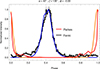 |
Fig. 2. Example of a good fit of the γ-ray pulse profile (≥0.1 GeV). The radio profile is shown in red, our model is displayed in orange, the γ-ray light curve is in black, and its fit is in blue. |
We checked the quality of the fit by the value of the reduced χ2, as shown in Fig. 3. The minimum value is around 1.3, and the uncertainties in the angles α and ζ are about 5°. However, we note that because the γ-ray light curve is invariant with respect to the change α → π − α and because we later discuss the radio polarisation fits, we decided to plot the χ2 values in the mirror symmetric region for α > 90°.
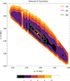 |
Fig. 3. Colour map showing the isocontours of the reduced χ2 fit for the γ-ray light curve for the angles α and ζ. The 1σ, 2σ, and 3σ confidence intervals are also shown. The minimum is located at (α, ζ) = (138° ,136° ) (corresponding to the mirror angle α = 42°) and depicted by a red circle. |
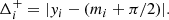
3.2. Dipole geometry from X-ray pulsations
In this section, we focus on the X-ray data interpretation. We summarise the findings of Choudhury et al. (2024) in Table 1 for their credible interval (CI) estimate and their maximum likelihood (ML) value. The subscripts p and s stand for primary and secondary hot spot. See Pétri (2017) for the definition of the angles (α, β, δ) and the displacement ϵ. Uncertainties about the given angles are about 0.05 rad, thus about 3°. The hot spots are non-antipodal and could correspond to an off-centred dipole. The geometry of this plausible dipole with parameters (α, β, δ, ϵ; see Pétri 2017, for the definition of these angles and ϵ) was then deduced and is shown in the right columns in the same Table 1. We found a mildly off-centred structure with a displacement d such that ϵ = d/R ≈ 0.36 − 0.46 and an obliquity of about α = 20° −26°. This is, however, 15° to 20° less than the magnetic obliquity α found by γ-ray light-curve fitting, although the inclination angle is within 1° of the radio measurements (Reardon et al. 2024) used in the NICER analyses. Nevertheless, the uncertainties in the location of the centre of the hot spot amounts to several degrees, thus allowing for some freedom, and they could increase the expected inclination of the equivalent magnetic dipolar axis to remain consistent with the γ-ray light-curve predictions.
Off-centred dipole geometry deduced from the polar cap location after the new joint NICER and XMM-Newton results of Choudhury et al. (2024).
Taking into account the oblate shape and the associated gravitational field could have an impact on the above results. Cadeau et al. (2007) showed that for spin frequencies above 300 Hz, large deviations from the correct X-ray light curve are expected if a spherical star is used (see also Morsink et al. 2007 for the impact of oblateness). This should be accurately quantified, but doing so is outside the scope of this work.
The annular shape of the northern hot spot found from the NICER data analyses (Choudhury et al. 2024) could be produced by a small-scale dipole underneath the surface, as shown in Fig. 4. This is an alternative to the dipole plus quadrupole geometry presented in other works (Gralla et al. 2017). In order to recover the size and thickness of this annular ring, the strength and precise location of this small-scale dipole must be adjusted. However, we do not dive into such details, as they do not provide more information about the multi-wavelength emission since this pole is not detected in radio.
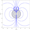 |
Fig. 4. Example of a dipole producing an annular hot spot on one pole. Magnetic field lines are shown in blue and the neutron star surface is shown as a solid black circle of normalised radius. The stellar interior is shown in light grey. |
3.3. Radio pulse profile
To go further in our understanding of the emission location and geometry, we investigated the features of the radio pulse profile. Starting with the pulse width (W) related to the beam cone half-opening angle (ρ) by (Gil et al. 1984),
 (1)
(1)
we estimated the cone opening angle to be ρ ≈ 80°, assuming α = 42°, ζ = 136°, and a pulse width of 80% of the period, and thus W = 0.8 × 2π. For a pure static dipole, this angle is related to the colatitude (θ) at which the radio beam is formed by
 (2)
(2)
Therefore, θ ≈ 53°, and the emission height becomes h/rL ≈ sin2θ ≈ 0.64, thus representing a substantial fraction of the light-cylinder radius. We can better estimate the emission height by computing the separatrix surface deduced from the force-free model and projecting the tangent to the field lines onto the sky. The result is shown in Fig. 5 for α = 42°. The magnetic axis is located at phase 0.5 and shown as a vertical dashed line, whereas the line of sight at ζ = 136° is shown as a horizontal dashed line. Each coloured line corresponds to a constant length (s) along a field line starting at the stellar surface and given in units of rL. We note that this length does not correspond to the usual emission altitude (h) reported in other works, as field lines are curved and not straight in the radial direction. The arc length (s) is measured in the neutron star corotating frame and starts with s = 0 at the neutron star surface, whereas h starts at the star centre, and thus h = R corresponds to s = 0. The curve asymmetry in Fig. 5 originates mainly from the electric current induced by the plasma flow and by the magnetic field sweep-back.
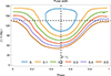 |
Fig. 5. Projection of the emission cone rims onto the sky for different emission lengths (s) in units of rL. The phase location of the magnetic axis at 0.5 is shown as a vertical dashed line, whereas the line of sight at ζ = 136° is shown as a horizontal dashed line. |
The evolution of the pulse width with respect to this curvilinear abscissa is shown in Fig. 6 in blue for the force-free (FFE) case and in red for the vacuum (VAC) case. The pulse width is a monotonically increasing function of the emission length (s), and a pulse width of 80% with W = 0.8 × 2π requires a length of about s/rL = 0.4 and thus a height of h/rL ≈ 0.5, which is slightly less than the pure dipole estimates. Above s/rL = 0.5, the pulse duty cycle becomes 100% and is visible for the full period of the pulsar. Figure 5 demonstrates that detecting pulsations for a significant fraction of the period, of almost 100%, does not require an almost aligned rotator for these pulsar parameters, especially for stars with fast rotation.
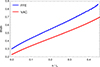 |
Fig. 6. Width of the radio pulse profile depending on the emission height (s) above the stellar surface along the magnetic field lines in units of rL for α = 42° and ζ = 136°. Blue is for the FFE case, and red is for the VAC case. |
3.4. Radio polarisation
To strengthen our estimate of the magnetic obliquity and line of sight inclination angles, we conclude this study by including radio polarisation data as observed for instance by Osłowski et al. (2014) and Dai et al. (2015). Multi-frequency polarisation pulse profiles are available at wavelengths of 10 cm (3.1 GHz), 20 cm (1.4 GHz), and 50 cm (0.7 GHz) with the associated PPA from the EPN database website. At 50 cm, the evolution is rather monotonic, with only two or three OPM switching events. At 20 cm, the smoothness becomes less obvious with a stronger OPM, and at 10 cm the PPA becomes much more erratic. This shift from a well-behaved PPA at low frequency to a much less well-structured PPA at high frequency hints at a decrease in the emission height when increasing the radiation frequency, in agreement with the radius-to-frequency mapping picture. A lower altitude means stronger multipolar components and therefore possibly a significant deviation from the RVM expectations. Nevertheless, we fit the rotating vector model of Radhakrishnan & Cooke (1969), who gave the time evolution of the linear polarisation angle (ψ) as
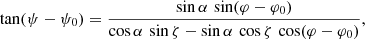 (3)
(3)
where ψ0 corresponds to the position angle of the spin axis on the plane of the sky and φ is the rotational phase (φ0 is a reference phase corresponding to the inflexion point, obtained by fitting the polarisation to the RVM expectations).
Neglecting the presence of OPMs would lead to bad fits to the PPA, and identifying the OPM jumps or simply removing them ‘by eye’ is not satisfactory. Therefore, we designed a fitting method that automatically incorporates variations of ±90° into the fitting scheme. To achieve our goal, we introduced a distance d(yi, mi) between the observations yi and model mi for each bin i such that
 (4a)
(4a)
 (4b)
(4b)
 (4c)
(4c)
This distance takes into account the periodicity of 180° (π rad) of the PPA as well as OPM switching for each bin. The values yi and mi are forced to stay in the interval [0, π] during the computation. We then minimised the following cost function, a kind of χ2 function defined by
 (5)
(5)
It automatically identifies the number of OPM jumps and their phase locations. The term σi represents the uncertainties in the polarisation angle in each bin (i). Actually, because PSR J0437−4715 is very bright in the radio, these uncertainties are tiny in general, less than 1° and even less than 0.1° in some phase bins. We therefore did not expect to obtain good reduced χ2 numbers close to unity because of the OPMs and small structures in the PPA. Moreover, since a low degree of linear polarisation Πi = Li/Ii (Ii is the total intensity Stokes parameter, and  is the linear polarisation intensity obtained from Qi and Ui Stokes parameters in each bin, i) makes it difficult to distinguish between the two orthogonal modes, we imposed a threshold on Πi to improve the distinction between the OPMs. We also modified the uncertainties σi to be weighted uncertainties related to the degree of linear polarisation Πi such that σi is replaced by σi′ − 1 = Ii Πi = Li, thus focusing on bright and highly linearly polarised bin phases. We typically set Πi = 20%−50%, removing data points below this threshold. We also enforced a threshold for the inflexion point such that sin α ≥ 2 sin(α − ζ) > 0 in order to constrain the derivative of the PPA to have the right trend with phase. This is particularly useful at a high polarisation Πi threshold, where data points are almost absent in the middle of the pulse profile. The resulting fits using the modified χ2 approach, Eq. (5), were therefore performed only on a subset of the total observational data, as shown in Fig. 7 where bins with polarisation degree Πi < 30% have been removed. The orange and green data points show the PPA when shifted by ±90° to simulate OPMs. The RVM shows a reasonable fit to the data with αrvm = 132° −149° and ζrvm = 114° −143° at different wavelengths of 10 cm, 20 cm, and 50 cm. The exact values of the fitting for the different wavelengths are reported in Table 2. We note that αrvm is the supplementary to α because we focus on the South Pole for polarisation purposes. Following the γ-ray light-curve fitting value, we should get αrvm ≈ π − α ≈ 180° −42° = 138°. Our values in Table 2 are consistent with this guess, within the uncertainties, and with earlier radio polarisation investigations by Manchester & Johnston (1995) who found α = 145° and ζ = 140°.
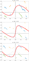 |
Fig. 7. Polarisation position angle as a function of rotational phase for PSR J0437−4715 as measured with the Parkes telescope at 10 cm, 20 cm, and 50 cm (top to bottom panels). Bins with a polarisation degree Πi < 30% have been removed. The best values for the PPA fits from the RVM are reported in Table 2. The radio pulse profile is shown in grey for better identification of the pulse. The RVM fit is shown with a solid red line. |
Values of the radio pulse width at 10% maximum intensity, obliquity (α), line of sight (ζ), phase shift (φ0), and offset (ψ0) obtained from RVM fits at different wavelengths and with minimum polarisation bins Πi > 30%.
3.5. Combined γ and radio fit
As a last step, we combined our γ and radio fits in a weighted total χ2 value given by
 (6)
(6)
Because χγ2 and χr2 usually have very different values, we adjusted the weights (wγ and wr) such that the two χ2 contribute equally at their respective minimum. In other words, we chose wγ = 1/min(χγ2) and wr = 1/min(χr2) to avoid the dominance of one wavelength over the other. A summary of the joint best fit is given in the last two columns of Table 2, and the combined χ2 maps are shown in Fig. 8 for the three wavelengths at 10 cm, 20 cm, and 50 cm. If the γ-ray fit is combined with the radio polarisation fit, for instance at the 50 cm wavelength, we obtain the best compromise between the radio polarisation and the γ-rays by averaging the obliquity and line of sight angles such that (α, ζ)≈(141° ,132° ). The impact of this geometry onto the PPA evolution is plotted in Fig. 9 at 50 cm.
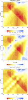 |
Fig. 8. Combined radio and γ-ray χ2 maps of Eq. (6) at the three wavelengths at 10 cm, 20 cm and 50 cm, from top to bottom. |
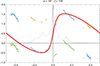 |
Fig. 9. Best joined radio/γ-ray fit with (α, ζ) = (141° ,132° ). This fit is to be compared with the bottom panel of Fig. 7, where bins with a linear polarisation degree less than Πi < 30% have been removed. |
4. Conclusions
Although MSP emission is usually thought to be difficult to model with a dipolar magnetic field because of the impact of multipolar components close to the stellar surface, we have shown that a modified dipole confidently reproduces a wealth of multi-wavelength properties of PSR J0437−4715. Independent determinations of the viewing angle agree to very good accuracy with ζ = (136 ± 5)°. Even the radio polarisation data are satisfactorily fitted with the RVM, and a large duty cycle in radio does not imply an almost aligned rotator. All of these results give us confidence in the reliability of γ-ray light-curve fitting within the striped wind framework, even for MSPs. This work supports once more the idea that two off-centred dipoles can satisfactorily reproduce the multi-wavelength feature of NICER pulsars as well as the hot spot geometry (Pétri et al. 2023, 2025). Several other NICER pulsars, such as PSR J1231−1411 and PSR J0614−3329, will be investigated with the method presented in this work in order to improve our understanding of MSP magnetic field structure and geometry.
To constrain the radio part of the spectrum even more firmly, a single pulse study would greatly benefit the radio polarisation fit, as suggested by Mitra et al. (2023). Such a study should keep only those pulses that are highly linearly polarised. PSR J0437−4715 is a very bright radio pulsar, so a single-pulse study of it should be possible, and we emphasise again that a joint radio and γ-ray fit offers a very promising avenue to better understand MSP radio emission mechanisms.
Acknowledgments
We are grateful to the referee for helpful comments and suggestions. This work has been supported by the ANR (Agence Nationale de la Recherche) grant number ANR-20-CE31-0010. SG and PS acknowledge the support of the CNES. Part of this research has made use of the EPN Database of Pulsar Profiles maintained by the University of Manchester, available at: https://psrweb.jb.man.ac.uk/epndb/
References
- Abdo, A. A., Ackermann, M., Ajello, M., et al. 2009, Science, 325, 848 [NASA ADS] [CrossRef] [Google Scholar]
- Becker, W., & Trümper, J. 1993, Nature, 365, 528 [Google Scholar]
- Bogdanov, S. 2013, ApJ, 762, 96 [Google Scholar]
- Bogdanov, S., Guillot, S., Ray, P. S., et al. 2019, ApJ, 887, L25 [NASA ADS] [CrossRef] [Google Scholar]
- Cadeau, C., Morsink, S. M., Leahy, D., & Campbell, S. S. 2007, ApJ, 654, 458 [Google Scholar]
- Carrasco, F., Pelle, J., Reula, O., Viganò, D., & Palenzuela, C. 2023, MNRAS, 520, 3151 [NASA ADS] [CrossRef] [Google Scholar]
- Chen, A. Y., Yuan, Y., & Vasilopoulos, G. 2020, ApJ, 893, L38 [Google Scholar]
- Choudhury, D., Salmi, T., Vinciguerra, S., et al. 2024, ApJ, 971, L20 [NASA ADS] [CrossRef] [Google Scholar]
- Dai, S., Hobbs, G., Manchester, R. N., et al. 2015, MNRAS, 449, 3223 [NASA ADS] [CrossRef] [Google Scholar]
- Dittmann, A. J., Miller, M. C., Lamb, F. K., et al. 2024, ApJ, 974, 295 [NASA ADS] [CrossRef] [Google Scholar]
- Dyks, J. 2019, MNRAS, 488, 2018 [NASA ADS] [CrossRef] [Google Scholar]
- Gil, J., Gronkowski, P., & Rudnicki, W. 1984, A&A, 132, 312 [NASA ADS] [Google Scholar]
- González-Caniulef, D., Guillot, S., & Reisenegger, A. 2019, MNRAS, 490, 5848 [NASA ADS] [CrossRef] [Google Scholar]
- Gralla, S. E., Lupsasca, A., & Philippov, A. 2017, ApJ, 851, 137 [NASA ADS] [CrossRef] [Google Scholar]
- Guillot, S., Kaspi, V. M., Archibald, R. F., et al. 2016, MNRAS, 463, 2612 [Google Scholar]
- Huang, C. 2026, ApJ, 999, 204 [Google Scholar]
- Huang, C., & Chen, A. Y. 2025, ApJ, 991, 90 [Google Scholar]
- Johnston, S., Lorimer, D. R., Harrison, P. A., et al. 1993, Nature, 361, 613 [NASA ADS] [CrossRef] [Google Scholar]
- Kalapotharakos, C., Wadiasingh, Z., Harding, A. K., & Kazanas, D. 2021, ApJ, 907, 63 [NASA ADS] [CrossRef] [Google Scholar]
- Lockhart, W., Gralla, S. E., Özel, F., & Psaltis, D. 2019, MNRAS, 490, 1774 [NASA ADS] [CrossRef] [Google Scholar]
- Lorange, A., Pétri, J., Sautron, M., & Vigon, V. 2026, A&A, 707, A395 [NASA ADS] [CrossRef] [EDP Sciences] [Google Scholar]
- Manchester, R. N., & Johnston, S. 1995, ApJ, 441, L65 [Google Scholar]
- Mauviard, L., Guillot, S., Salmi, T., et al. 2025, ApJ, 995, 60 [Google Scholar]
- Miller, M. C., Lamb, F. K., Dittmann, A. J., et al. 2019, ApJ, 887, L24 [Google Scholar]
- Miller, M. C., Lamb, F. K., Dittmann, A. J., et al. 2021, ApJ, 918, L28 [NASA ADS] [CrossRef] [Google Scholar]
- Mitra, D., Melikidze, G. I., & Basu, R. 2023, MNRAS, 521, L34 [Google Scholar]
- Morsink, S. M., Leahy, D. A., Cadeau, C., & Braga, J. 2007, ApJ, 663, 1244 [NASA ADS] [CrossRef] [Google Scholar]
- Navarro, J., Manchester, R. N., Sandhu, J. S., Kulkarni, S. R., & Bailes, M. 1997, ApJ, 486, 1019 [Google Scholar]
- Osłowski, S., van Straten, W., Bailes, M., Jameson, A., & Hobbs, G. 2014, MNRAS, 441, 3148 [Google Scholar]
- Pavlov, G. G., & Zavlin, V. E. 1997, ApJ, 490, L91 [NASA ADS] [CrossRef] [Google Scholar]
- Pétri, J. 2017, MNRAS, 466, L73 [CrossRef] [Google Scholar]
- Pétri, J., Guillot, S., Guillemot, L., et al. 2023, A&A, 680, A93 [NASA ADS] [CrossRef] [EDP Sciences] [Google Scholar]
- Pétri, J., Guillot, S., Guillemot, L., et al. 2025, A&A, 701, A39 [NASA ADS] [CrossRef] [EDP Sciences] [Google Scholar]
- Radhakrishnan, V., & Cooke, D. J. 1969, Astrophys. Lett., 3, 225 [NASA ADS] [Google Scholar]
- Reardon, D. J., Bailes, M., Shannon, R. M., et al. 2024, ApJ, 971, L18 [Google Scholar]
- Riley, T. E., Watts, A. L., Bogdanov, S., et al. 2019, ApJ, 887, L21 [Google Scholar]
- Salmi, T., Vinciguerra, S., Choudhury, D., et al. 2022, ApJ, 941, 150 [CrossRef] [Google Scholar]
- Salmi, T., Deneva, J. S., Ray, P. S., et al. 2024, ApJ, 976, 58 [Google Scholar]
- Smith, D. A., Abdollahi, S., Ajello, M., et al. 2023, ApJ, 958, 191 [NASA ADS] [CrossRef] [Google Scholar]
- Sur, A., Yuan, Y., & Philippov, A. 2024, ApJ, 965, 140 [Google Scholar]
- Vinciguerra, S., Salmi, T., Watts, A. L., et al. 2024, ApJ, 961, 62 [NASA ADS] [CrossRef] [Google Scholar]
- Zavlin, V. E. 2006, ApJ, 638, 951 [NASA ADS] [CrossRef] [Google Scholar]
- Zavlin, V. E., & Pavlov, G. G. 1998, A&A, 329, 583 [NASA ADS] [Google Scholar]
- Zavlin, V. E., Pavlov, G. G., Sanwal, D., et al. 2002, ApJ, 569, 894 [Google Scholar]
All Tables
Off-centred dipole geometry deduced from the polar cap location after the new joint NICER and XMM-Newton results of Choudhury et al. (2024).
Values of the radio pulse width at 10% maximum intensity, obliquity (α), line of sight (ζ), phase shift (φ0), and offset (ψ0) obtained from RVM fits at different wavelengths and with minimum polarisation bins Πi > 30%.
All Figures
|
Fig. 1. Multi-wavelength pulse profile of PSR J0437−4715 as observed in the radio by Parkes at 1.4 GHz (red line), in soft X-rays by NICER (0.3−3.0 keV, green line), and in γ-rays by Fermi/LAT (black line). Note that the zero line of the NICER data is arbitrary since, technically, the pulsed emission lies on top of an un-pulsed pulsar emission plus background emission (all origins combined). We note that this is also true for the radio data, for which the profile baseline has been subtracted to lie at zero. |
| In the text | |
|
Fig. 2. Example of a good fit of the γ-ray pulse profile (≥0.1 GeV). The radio profile is shown in red, our model is displayed in orange, the γ-ray light curve is in black, and its fit is in blue. |
| In the text | |
|
Fig. 3. Colour map showing the isocontours of the reduced χ2 fit for the γ-ray light curve for the angles α and ζ. The 1σ, 2σ, and 3σ confidence intervals are also shown. The minimum is located at (α, ζ) = (138° ,136° ) (corresponding to the mirror angle α = 42°) and depicted by a red circle. |
| In the text | |
|
Fig. 4. Example of a dipole producing an annular hot spot on one pole. Magnetic field lines are shown in blue and the neutron star surface is shown as a solid black circle of normalised radius. The stellar interior is shown in light grey. |
| In the text | |
|
Fig. 5. Projection of the emission cone rims onto the sky for different emission lengths (s) in units of rL. The phase location of the magnetic axis at 0.5 is shown as a vertical dashed line, whereas the line of sight at ζ = 136° is shown as a horizontal dashed line. |
| In the text | |
|
Fig. 6. Width of the radio pulse profile depending on the emission height (s) above the stellar surface along the magnetic field lines in units of rL for α = 42° and ζ = 136°. Blue is for the FFE case, and red is for the VAC case. |
| In the text | |
|
Fig. 7. Polarisation position angle as a function of rotational phase for PSR J0437−4715 as measured with the Parkes telescope at 10 cm, 20 cm, and 50 cm (top to bottom panels). Bins with a polarisation degree Πi < 30% have been removed. The best values for the PPA fits from the RVM are reported in Table 2. The radio pulse profile is shown in grey for better identification of the pulse. The RVM fit is shown with a solid red line. |
| In the text | |
|
Fig. 8. Combined radio and γ-ray χ2 maps of Eq. (6) at the three wavelengths at 10 cm, 20 cm and 50 cm, from top to bottom. |
| In the text | |
|
Fig. 9. Best joined radio/γ-ray fit with (α, ζ) = (141° ,132° ). This fit is to be compared with the bottom panel of Fig. 7, where bins with a linear polarisation degree less than Πi < 30% have been removed. |
| In the text | |
Current usage metrics show cumulative count of Article Views (full-text article views including HTML views, PDF and ePub downloads, according to the available data) and Abstracts Views on Vision4Press platform.
Data correspond to usage on the plateform after 2015. The current usage metrics is available 48-96 hours after online publication and is updated daily on week days.
Initial download of the metrics may take a while.