| Issue |
A&A
Volume 708, April 2026
|
|
|---|---|---|
| Article Number | A338 | |
| Number of page(s) | 10 | |
| Section | Stellar structure and evolution | |
| DOI | https://doi.org/10.1051/0004-6361/202557759 | |
| Published online | 23 April 2026 | |
Magnesium isotopic detection in cool stars: Tracing nucleosynthetic signatures from MgH features
University of Canterbury, Private Bag 4800, Christchurch 8140, New Zealand
★ Corresponding author: This email address is being protected from spambots. You need JavaScript enabled to view it.
Received:
20
October
2025
Accepted:
14
February
2026
Abstract
Context. Magnesium isotopic ratios offer valuable insights into stellar nucleosynthesis and Galactic chemical evolution, particularly in distinguishing between contributions from supernovae and asymptotic giant branch (AGB) stars. These isotopes are accessible through MgH molecular features in cool stellar atmospheres, yet their measurement remains challenging across a range of spectral types.
Aims. We aim to assess the reliability of MgH spectral regions for extracting magnesium isotopic ratios (24Mg, 25Mg, and 26Mg) in stars spanning spectral types from M to G, and to evaluate the consistency of these measurements with nucleosynthetic expectations.
Methods. We applied an analysis pipeline using spectrum synthesis to derive isotopic ratios, validated using three well-studied reference stars, to a sample of five additional dwarf and giant stars. Individual MgH molecular band regions were analysed to determine their sensitivity to isotopic variation. Europium (Eu) and barium (Ba) abundances were also measured to explore potential correlations with magnesium isotopic ratios as r and s process proxies, respectively.
Results. There are ten wavelength regions for which MgH have previously been investigated. Our study determined that seven of these regions were the most reliable for extracting isotopic information. Other regions exhibited limited sensitivity between stellar type and parameters. The Mg isotope ratios (24Mg:25Mg:26Mg) obtained in this work include: HD 11695-81:7:12; HD 18884-81:7:12; HD 18907-69:9:23; HD 22049-71:16:13; HD 23249-66:13:22; HD 128621-67:17:16; HD 10700-78:10:12; and HD 100407-65:10:25. Comparison of europium (Eu) abundances with the three magnesium isotopes revealed strong correlations. The strongest correlation was with 24Mg. Note that 24Mg is predominantly produced by hydrostatic α capture in massive stars, a process that precedes the r process responsible for Eu production. In contrast, barium (Ba) abundances showed no significant correlation with 25Mg and 26Mg, despite their shared AGB origin. With removal of the effect of metallicity similar results were found.
Conclusions. Our results demonstrate that selected MgH regions can reliably measure magnesium isotopes in cool stars, providing a reproducible framework for future studies of stellar nucleosynthesis and galactic chemical evolution.
Key words: methods: observational / techniques: spectroscopic / stars: abundances / stars: fundamental parameters
© The Authors 2026
 Open Access article, published by EDP Sciences, under the terms of the Creative Commons Attribution License (https://creativecommons.org/licenses/by/4.0), which permits unrestricted use, distribution, and reproduction in any medium, provided the original work is properly cited.
This article is published in open access under the Subscribe to Open model. This email address is being protected from spambots. You need JavaScript enabled to view it. to support open access publication.
1. Introduction
The nucleosynthetic processes that occur within the later stages of stellar evolution are important for understanding element evolution in the Milky Way. During these processes various elements, and therefore various isotopes of each element, are created in multiple nucleosynthetic environments. Previous studies, Karakas & Lattanzio (2003), Iliadis (2007), Vangioni & Olive (2019) and Kobayashi et al. (2020), describe the nucleosynthetic origins of magnesium (Mg) isotopes, amongst other isotopes. There are four nucleosynthetic processes that we subsequently focus on: the α process; hot-bottom burning; the s process (slow neutron capture); and the r process (rapid neutron capture).
The α process is one of the main production channels for the 24Mg isotope. The hydrostatic α process occurs during the Carbon-, Neon-, and Oxygen-core-burning stages of massive stars (≤8 M⊙) and generates elements with an atomic number of multiples of four (Vangioni & Olive 2019; Iliadis 2007). Such massive stars often end their life as core-collapse supernovae, which is when this isotope is dispersed through the inter-stellar medium (ISM).
Hot-bottom burning occurs in the asymptotic giant branch (AGB) phase of intermediate mass stars (0.8–8 M⊙). At this stage the stars are hot enough for efficient proton capture by Mg leading to Al which then decays into heavier Mg isotopes. The 25, 26Mg isotopes are also produced during thermal pulses of helium shell burning. Note that α capture on 22Ne can lead to both 25Mg and 26Mg (Vangioni & Olive 2019) (in the 22Ne(α, n)25Mg and 22Ne(α, γ)26Mg reactions (Iliadis 2007)).
We note that s process nucleosynthesis occurs during the AGB phase in stars of mass range 0.5 to 8 M⊙. The 25Mg and 26Mg isotopes are mostly generated via hot-bottom burning, the products are then distributed into the inter-stellar medium (ISM), along with s process elements, via stellar winds (Vangioni & Olive 2019; Iliadis 2007; Karakas & Lattanzio 2003).
Supernovae and high-energy collisions, such as neutron star mergers, are where the r process nucleosynthesis occurs. Small amounts of 24Mg, 25Mg, and 26Mg can be generated by r process nucleosynthesis (Kobayashi et al. 2020).
Stars that we observe today formed from polluted material in the ISM, and bear the signatures of these different nucleosynthetic events. The isotopes of magnesium can be generated in multiple nucleosynthetic environments, determining the relative isotopic abundances allow us to distinguish between the nucleosynthetic channels that created the elements throughout time. Using isotopes to distinguish between these events allows for a deeper understanding of the history of the galaxy and its chemical evolution.
Magnesium isotope ratios can be measured from the magnesium hydride (MgH) molecular features present in stellar spectra. In this study, we examined a set of MgH features in order to derive the ratios of 24Mg, 25Mg, and 26Mg. The MgH molecules thermally dissociate due to the covalent bonds that hold the molecules together, which decay at high temperatures (Pavlenko et al. 2008). Using the Saha equation and a dissociation energy from Shayesteh et al. (2007), we calculated an effective temperature of Teff ≈ 5800 ± 300 K, which corresponds to an expected dissociation temperature. This provides a potential upper limit on the stellar effective temperature above which the MgH feature is unlikely to be detectable.
The Gaia benchmark stars (GBS) are well-studied, bright, or nearby stars of the late F, G, and K spectral types with a range of luminosities and metallicities (Heiter et al. 2015), making them ideal for examining MgH over a broad range of stellar parameters. The GBS dataset is well know in the galactic archaeology literature and has been widely used in spectroscopic surveys such as GALAH (Buder et al. 2021) and Gaia-ESO (Gilmore et al. 2022). The GBS were curated to be used to calibrate spectroscopic pipelines and make comparison of stellar parameters between spectroscopic surveys. The original set of GBS (V1/V2) contained 34 stars ranging in effective temperature from 4000 K to 6500 K which included FGKM giants, dwarfs, and subgiants. Given their well-characterised nature and broad coverage of stellar parameters, the GBS provided an ideal sample for determining Mg isotopes.
Previous studies of Mg isotope determination include McWilliam & Lambert (1985), Barbuy (1985), Barbuy (1987), McWilliam & Lambert (1988), Gay & Lambert (2000), Yong et al. (2003, 2004, 2006), Meléndez & Cohen (2009), Thygesen et al. (2016), McKenzie et al. (2024a), and McKenzie et al. (2024b). These works used a range of computational approaches, including differential analysis, manual isotope fitting, and χ2 fitting to compare synthetic spectra with observations (typically generated with MOOG; Sneden et al. 2012). Many of these studies focused on giant stars with a few focusing on cool dwarfs (Yong et al. 2003; McKenzie et al. 2024a). This study builds on these foundations, drawing on their insights into line list development, synthesis, and fitting techniques. To extend this work across a broader range of stellar parameters, we focus on the Gaia benchmark stars. All of these studies have focused on 1D determinations of Mg isotopes. However, several works have also investigated the 3D effects of MgH line formation and how 3D line asymmetries influence the inferred isotopic ratios. These studies aim to quantify how Mg isotope determinations in 3D differ from those obtained in 1D. In general, the impact on the isotopic ratios is small, but in some cases the differences become significant. When this occurs, 1D analyses can misestimate the isotopic ratios by up to 5 percentage points for 24Mg and 25Mg (Thygesen et al. 2017). While this distinction is not critical for the present study, it is worth noting.
This paper is structured as follows. Section 2 describes the observations and data processing. Section 3 details the measurement of magnesium isotopes and the underlying calculations. In Section 4, we assess the quality of the data produced by our pipeline, compare our results with literature values, and explore correlations between magnesium isotope abundances and neutron-capture elements. In Section 5 we engage in final discussions and conclusions.
2. Observations
Building on the strengths of the GBS, we selected a subset of stars observable from the University of Canterbury  teh
teh wai Mt John Observatory to investigate MgH features in detail. We used the High Efficiency and Resolution Canterbury University Large Echelle Spectrograph (HERCULES) instrument in this study. HERCULES is fibre-fed from the 1 m McLellan telescope (Hearnshaw et al. 2002; Hearnshaw 1986). We chose to use HERCULES to test the capabilities of the instrument with an R ∼ 82 000 to confirm if it was capable of isotope determination. The spectra were reduced using the in-house reduction pipelines MEGARA (Version 1.5)1 and DEIANIRA2.
Three observing runs of seven days, were conducted in February, June, and September of 2024. Figure 1 presents the GBS V3 catalogue (Soubiran et al. 2024) as a Kiel diagram, with the stars observed in this study indicated with circles.
 |
Fig. 1. Kiel diagram showing the distribution of ISAM stars in temperature space (circled), coloured by metallicity. The background points are the stars from GBS V3 (Soubiran et al. 2024) to show the main sequence more clearly. |
For this study 18 stars were observed, the details of which are shown in Table 1. In order to find Mg isotopes across the parameter space 16 of 18 stars from the GBS were selected that have spectral types ranging from M4 to F9 with both dwarf and giant stars included. Three other stars of F and G types were selected from the 5th catalogue of nearby stars (Golovin et al. 2023) as filler stars that were observable during observing runs. All stars in the Isotope Sample (ISAM) were brighter than V = 6, ensuring the highest signal-to-noise ratio achievable with a 1 m telescope. Between ten and 40 observations were taken for each star, combining observations with a median stack to further increase the signal-to-noise ratio, aiming for a final S/N of approximately 100. We use the modules developed in iSpec (Blanco-Cuaresma 2013) to perform the median-stacking, thereby maximising the likelihood of successfully extracting isotope information.
Derived stellar parameters for the ISAM.
2.1. Data processing
This section outlines the derivation of stellar parameters used to assess continuum normalisation in regions sensitive to MgH. We used the GBS V2 parameters (Jofré et al. 2015) to create our synthetic spectra, as they were derived using robust methods; however, careful continuum normalisation was still required to ensure an accurate comparison with observed spectra. We independently derived stellar parameters using the spectral synthesis tools iSpec (Blanco-Cuaresma et al. 2014) and MOOG (Sneden et al. 2012). The derived parameters were then compared to the GBS (V2) values, to check for consistency and confirm that the normalisation was valid. The parameters we derived include, effective temperature (Teff), surface gravity (log g), metallicity ([M/H]), projected rotational velocity (v sin i), and α-element abundance ([α/Fe]). These were iteratively adjusted within iSpec by fitting synthetic spectra to the observed data, allowing convergence on the best-fit values. This approach ensured that our analysis was aligned with established GBS parameters and that the spectra were prepared for isotope extraction.
We used the same methods as Jofré et al. (2015) to derive parameters, as described above, a comparison between the derived parameters and the GBS V2 values is shown in Table 1. For dwarf stars (log g > 3.2), there was good agreement, with all parameters falling within 3σ of the GBS values. For giant stars (log g < 3.2), the agreement was poorer, with discrepancies up to 5σ across all parameters. The disagreement between values was expected to some extent. Additionally, the parameters for HD 11695 and HD 157244 highlight a known limitation in iSpec (Blanco-Cuaresma et al. 2014) where convergence of parameters, particularly log g, can vary significantly. The cause of this limitation was not identified in this study or by Blanco-Cuaresma et al. (2014). However, since the majority of the sample lies within 3σ of the reference values for most parameters, we conclude that our continuum placement is sufficiently accurate to derive magnesium isotope abundances with reasonable confidence.
3. Measurement of Mg isotopes
3.1. MgH regions
In Table 2 we have listed 10 MgH features used for Mg isotope fitting from the literature. Regions 1, 2 and 3 were defined by McWilliam & Lambert (1985). Region 4 defined by Meléndez & Cohen (2009), 5 by Thygesen et al. (2016), and the remaining regions by McKenzie et al. (2024b). We evaluated each region for its reliability for extracting isotope abundances. Regions deemed unreliable were excluded from the analysis, as is discussed in Section 4.2.
Regions used for magnesium isotopic analysis.
3.2. Isotope pipeline
While recent isotopic measurements have focused on giant stars and globular clusters (McKenzie et al. 2024b), our study focuses on field giants and dwarfs, expanding the scope of magnesium isotope analysis. To support this, we developed a Python wrapper 3 for the MOOG spectral synthesis code (Sneden et al. 2012) that iteratively converges on a best-fit solution, following previous methodologies. Spectral synthesis is central to this process: the pipeline determines magnesium isotopic abundances by performing a χ2 test between the synthetic and observed spectrum across a range of macroturbulence velocities (Vmac) and relative abundances of each magnesium isotope. These parameters are varied simultaneously to identify the best fit.
To reduce degeneracy and isolate the isotopic signal, several stellar parameters were fixed during the analysis: effective temperature (Teff), surface gravity (log g), metallicity ([M/H]), projected rotational velocity (v sin i), and α-element abundance ([α/Fe]) were adopted from the literature (Jofré et al. 2015) for GBS and van Leeuwen et al. (2022) for non-GBS stars.
To find the abundances of Mg, europium (Eu) and barium (Ba) we used the standard spectrum fitting method. This process isolates spectral lines from the rest of the spectrum, fitting a synthetic spectra to each observed line using iSpec (Blanco-Cuaresma 2013). Each is checked visually for quality, and an average weighted by the uncertainty of the resulting abundances was calculated (see Section 3.2.2).
Global magnesium abundances were determined using eight Mg lines (see Table 3) selected from the Gaia-ESO survey that had quality flags of Y (yes) or U (uncertain or undecided), indicating suitability for reliable abundance measurements (Heiter et al. 2021). The derived Mg abundances show good agreement with literature values (see Table 6), with most stars falling within 2σ of the GBS (Jofré et al. 2015). Note that α Cet and τ Cet exhibit differences at the 3σ level. For α Cet, the discrepancy corresponds to a difference of 0.78 dex, although this remains within 3σ due to the relatively large uncertainties in both this work and the GBS reference value. In contrast τ Cet has a discrepancy of 0.12 dex. These results suggest that the Mg abundances derived here are generally robust.
Lines used for abundance determination.
For some MgH features, minor adjustments to the continuum placement were necessary due to blending with strong Fe and C features in the surrounding spectrum. The Fe abundance was fixed to the literature [M/H] value (Jofré et al. 2015), and the carbon abundance was determined. Note that CO and C2 abundances were adjusted manually to better fit the wings of some features, improving continuum placement and reducing computation time. This same procedure was applied to Ba and Eu abundances for the neutron-capture element comparison (see Section 4.4) using the lines listed in Table 3. To maintain consistency across elements, we used the Mg abundances derived in this work rather than relying on literature values, as reference abundances for Ba and Eu were not available for all stars.
Using the global Mg abundance, the individual isotopic abundances were calculated from the isotopic ratios using Equation 2. See Section 3.2.1 for more details.
With all other parameters fixed, only Vmac and the relative abundances of 24Mg, 25Mg, and 26Mg were allowed to vary. Note that Vmac accounts for large-scale turbulent motions in a star’s atmosphere that broaden spectral lines beyond the effects of thermal motion or rotation (Iliadis 2007). In spectral synthesis and line profile fitting, Vmac is a key parameter influencing the shape and depth of absorption features. Rather than fixing Vmac to a single value for each star, it was allowed to vary per feature to account for potential differences in how turbulence affects lines of different strengths, excitation potentials, or formation depths. The derived Vmac values agreed with typical values for stars of these spectral types (Gray 2005).
The isotope pipeline operates by exploring the surrounding parameter space from an initial starting point. A synthetic spectrum is generated using these initial values, and its χ2 is calculated against the observed spectrum. Beginning with Vmac, we sample nearby values in abundance space and identify the one that minimises the χ2. This value is then fixed, and the process is repeated sequentially for 24Mg, 25Mg, and finally for 26Mg, yielding a preliminary set of parameters. We continue this iterative sampling of neighbouring values in parameter space until the χ2 is minimised across all parameters, ensuring convergence on the final solution.
As an example, Figure 2 shows the best fit for region 1 of HD 18907. Individual panels illustrate the contribution of each Mg isotope, with the bottom right panel showing the final combined synthetic spectrum. Fits were evaluated only within the coloured region, following the same procedure used for general abundance analysis as described earlier in Section 3.2. The strongest contribution of the feature comes from 24Mg, which is why the isotope fitting process begins with 24Mg after Vmac.
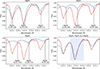 |
Fig. 2. Individual and combined contributions of Mg isotopes to region 1 of HD 18907. The top left panel shows the synthetic spectral feature from 24Mg only (no contribution from 25Mg or 26Mg). The top right panel shows the feature from 25Mg only, and the bottom left panel shows the 26Mg contribution. The bottom right panel with the fitting region in the blue box, presents the combined synthetic spectrum including all three isotopes, providing the best fit solution for this region. |
To minimise potential bias and ensure consistency across the sample, the same initial conditions were used for all stars. These consisted of the approximate solar Mg isotope ratio (De Bièvre & Barnes 1985) and the solar Vmac of Vmac = 8.41 km s−1 (McKenzie et al. 2024a). The initial isotope ratio was set to 24Mg:25Mg:26Mg = 77.69:10.36:11.95 (approximately 2:15:13 in MOOG input), as reported by McKenzie et al. (2024a).
We implement a two-stage fitting approach (coarse and fine) to avoid the solution becoming trapped in a local minimum, which could prevent convergence to the correct isotopic abundances. Using a large initial step allowed the solution to approach the global minimum, and then a finer step refined the isotopic abundances to better represent the observed spectrum. The first iteration used coarse steps (0.5) for the 24Mg inverse abundance (inverse abundance relative to the isotopic abundance for MOOG), followed by a finer search with steps of 0.1 to refine the fit.
This refinement was applied only to 24Mg because it is the dominant isotope and contributes most significantly to the MgH molecular features in the spectrum. Due to its stronger influence on the overall line strength and profile, small changes in 24Mg abundance have a more noticeable effect on the fit quality. In contrast, the contributions from 25Mg and 26Mg are minor and primarily affect the shape of the line profile rather than its depth. Once an optimal value for 24Mg was determined, the sensitivity of the fit to changes in 25Mg and 26Mg was reduced, making a coarse search unnecessary for those isotopes.
Although the isotopic ratios derived from different features within a star did not always agree precisely, they generally clustered around a consistent range. For each iteration, the χ2 values, resulting isotope ratios, and the fit between the observed and synthetic spectra were visually inspected to ensure they made physical sense.
On a per star basis, a spectral region was removed from consideration if any of four conditions were met: the synthetic spectrum did not match the depth of the observed spectrum; the isotope ratios were different by more than 3σ with those from other MgH regions in the same star; the 24Mg ratio differed by more than 25% from other regions; and the 25Mg and 26Mg isotopes were not approximately equal (as these isotopes tend to be produced together in similar amounts (Iliadis 2007)). Additionally, if the core of the molecular feature was well fitted but the wings deviated beyond the fitting region, the line was considered with caution.
After applying these criteria, a final check of the χ2 was performed to ensure the fit was minimised as much as possible. A difference of up to 25% in the 24Mg fraction was considered acceptable in order to retain as many regions as possible; however, up to 25% may cause the final isotopic ratio for each star to diverge from the ‘true’ isotope ratio. Therefore, this condition was applied carefully and only when evaluating a small number of successfully fitted regions. This approach allowed us to derive robust isotopic ratios across the sample, while accounting for blending, continuum placement, and fitting uncertainties.
3.2.1. Calculating Mg isotopic abundances
The isotope pipeline determines a ratio for all three isotopes from a predetermined global magnesium abundance. To convert the isotope ratio into individual isotopic abundances, we first calculate the relative ratios of the three Mg isotopes using the inverse ratio approach,
 (1)
(1)
where ik represents the measured isotope value for isotope k, expressed as an inverse abundance represented as a fraction of the isotope over the total Mg (e.g. i24 = 2 for 24Mg). The term  converts the percentage ratio into a scaled inverse value, which reflects the relative contribution of isotope k in the normalisation process. The denominator sums these scaled inverse abundances over all magnesium isotopes (j ∈ 24, 25, 26), ensuring proper normalisation. The final result is multiplied by 100 to express Rk as a percentage of the total magnesium isotopic composition. This formulation ensures that the three ratios R24, R25, and R26 sum to 100%.
Once the isotope ratios are determined, the individual isotopic abundances for each star are calculated using,
![Mathematical equation: $$ \begin{aligned}{[\text{ Mg}_i/\text{ H}]} = {[\text{ Mg}/\text{ H}]} + \log _{10}\left( \frac{f_i^{*}}{f_i^{\odot }} \right), \end{aligned} $$](/articles/aa/full_html/2026/04/aa57759-25/aa57759-25-eq5.gif) (2)
(2)
where fi* is the fraction of magnesium in isotope i in the star, and fi⊙ is the corresponding fraction in the Sun and [Mg/H] is the global abundance of Mg relative to solar. The same equation is used to propagate the uncertainty.
3.2.2. Uncertainty estimation
Uncertainties in the isotopic abundances were estimated using the Hessian matrix, which captures the gradients of the χ2 surface around the best-fit solution. The matrix was constructed by evaluating the second derivatives of Vmac, and the inverse abundances of 24Mg, 25Mg, and 26Mg. To compute these derivatives, each parameter was incrementally shifted up and down, and the resulting change in χ2 was used to assess the local curvature. Once the Hessian was assembled, its inverse was taken to obtain the covariance matrix, with the square root of the diagonal elements providing the uncertainties.
This method is sensitive to the choice of step size: if the shifts are too large or too small, the matrix can become numerically unstable, leading to inflated uncertainties (Cowan 1998). The most stable configuration was found to be: Vmac = 0.0001, i24 = 0.05, i25 = 0.1, and i26 = 0.1. These values produced consistent and stable uncertainty estimates across all fitted regions.
To convert uncertainties in inverse isotope ratios to actual isotope ratios, we applied the transformation described in Equations (4)–(6), which define the propagation of uncertainty through the inverse ratio formulation.
In addition, uncertainties in the stellar parameters and abundances were computed using iSpec, which applies a non-linear least-squares fitting algorithm (Levenberg–Marquardt) (Blanco-Cuaresma et al. 2014). iSpec automatically computes a covariance matrix during fitting, providing a fast and reliable estimate of parameter uncertainties.
The calculation of uncertainties in the magnesium isotope ratios follows from the inverse ratio formulation used in MOOG. These uncertainties are derived from the Hessian matrix and propagated through the ratio transformation.
The inverse ratio term is defined as,
 (3)
(3)
The uncertainty for each isotope is calculated as,
 (4)
(4)
where ik is the MOOG-derived ratio for isotope k, and σik is its uncertainty from the Hessian matrix of each isotope.
The uncertainty in the total inverse sum (σS) is then,
 (5)
(5)
where S is  .
.
The normalised isotope ratios are computed as,
as described in Equation 1.
Finally, the uncertainty in each ratio is propagated using,
 (6)
(6)
This formulation ensures that uncertainties in the fitted inverse abundances are accurately reflected in the final isotopic ratios, maintaining consistency with the MOOG fitting framework.
3.3. MgH lines in FGK spectra
Figure 3 shows the 10 MgH regions described in Section 3.1, colour-coded by temperature. It illustrates how the MgH features vary across stars of different temperatures: in the hottest star (lighter colours), HD 156098 (Teff = 6273 K; van Leeuwen et al. 2022), the features are either very weak or have vanished entirely, whereas in the coolest star (darker colours), HD 11695 (Teff = 3362 K; Jofré et al. 2015), they are much stronger. On the basis of this, a temperature cut-off was identified, above which the isotope pipeline cannot reliably measure magnesium isotopes using the devised methods. This limit is approximately ∼5400 K, meaning that for nearly all stars hotter than this threshold (primarily G and F type stars) these MgH regions are not viable for determining the Mg isotope abundances using our method. The value of ≈5800 ± 300 K, that we calculated in Section 1 is higher than the observational limit determined in this study. Our dataset includes stars, both above and below this temperature range, for which reliable Mg isotope measurements could not be obtained. This suggests that additional factors may influence detectability, such as log g, where higher gravity promotes molecular formation, and metallicity or Mg abundance can increase the depth of the spectral features (Gray 2005).
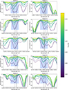 |
Fig. 3. Regions 1 through 10 showing the MgH lines and the fitting region (blue shaded rectangle) for all stars colour coded by effective temperature. Vertical lines mark the positions of the three magnesium isotopes: dot–dash for 24Mg, dashed for 25Mg, and solid for 26Mg. |
4. Analysis and discussion
4.1. Analysis pipeline verification
This study involved a multi-stage analysis with several iterations and refinements. At each stage, and whenever a new star was added to the sample, we reviewed the pipeline and applied the insights gained, leading to the removal of some regions after assessing their performance across all stars. To assess the reliability of the final version of our isotope analysis pipeline, we compared our results for three stars with published magnesium isotope measurements: τ Ceti (HD 10700), α Centauri B (HD 128621), and δ Eridani (HD 23249). Isotopic ratios were determined using a χ2 minimisation approach across multiple regions (Table 2), followed by visual inspection of the observed and synthetic spectra. The median weighted averages across all regions were then computed to produce the final isotopic ratios.
In Table 4, we compare the magnesium isotope ratios derived in this study with the values reported in the literature for three reference stars, as well as for stars with similar stellar parameters. Our result for τ Ceti is consistent with the range of literature values with all three isotopes within uncertainty of at least one of the reference values. Deviations are seen in α Centauri B and δ Eri, with differences of up to 13% (of total abundance) for 24Mg and 11% for 26Mg. These differences may arise from our use of a larger number of spectral regions, which provides a broader sampling of isotopic features. Additionally, extracting isotopic ratios for the two dwarf reference stars is challenging, as they lie near the upper Teff limit of the pipeline. Additional literature values were included for comparison, featuring three K-type stars, one G-type star, and one giant star with similar stellar parameters to our targets. The comparison stars are similarly distributed in magnesium isotope parameter space, making them suitable analogues for assessing the consistency and reliability of our measurements.
Mg isotope ratios found in this study compared to the literature.
Overall, agreement with the literature is reasonable (see Table 4), particularly considering that earlier studies relied on manual fitting techniques and smaller number of regions. Previous studies either did not specify which spectral regions were used or focused solely on Regions 1–3 (Gay & Lambert 2000), whereas this work includes Regions 1, 3, 5, 6, 8, 9, and 10. Region 2 and 4 were excluded due to contamination by strong atomic lines in the nearby continuum. The inclusion of additional regions and the use of a χ2-based fitting procedure likely contributed to the robustness of the derived isotopic ratios. However, direct comparison with the literature is limited by the lack of methodological detail in previous studies, particularly regarding their fitting procedures and continuum treatment. As such, the reliability of our results is best assessed through internal consistency checks and the quality of the fits across multiple regions.
4.2. Region quality check
Figure 4 shows the isotopic fraction of each magnesium isotope as a function of region wavelength. Each point corresponds to the central wavelength of a region, and the vertical error bars indicate the range of isotopic fraction across the sample. Regions 1, 2 and 3 were used primarily in previous studies (Gay & Lambert 2000; Yong et al. 2003, 2004); however, region 2 was excluded in this work due to poor performance. Regions 8 and 10 both have large standard deviations, reflecting significant variation between stars with different magnesium abundances. Regions 1, 5, 6 and 9 show a similar amount of scatter, suggesting they are good for measuring isotope ratios. In contrast, regions 2, 3, 4 and 7 have very little scatter, meaning they are less sensitive to differences in the metallicity, log g and Teff of the stars. It is likely the largest factor in this variation is Teff as discussed in Section 3.3. For the ISAM, we recommend using regions 1, 5, 6, 8, 3, 9 and 10 for deriving robust isotopic ratios.
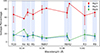 |
Fig. 4. Mean isotopic percentage as a function of region wavelength for 24Mg (red), 25Mg (blue), and 26Mg (green). Error bars indicate the standard deviation of the ISAM for each region. |
4.3. Magnesium isotopes
The isotopic ratios determined for the eight stars in this study are presented in Table 5. The results are consistent with various literature sources, as shown in Table 4.
Isotope ratios for the ISAM.
The pipeline failed to produce a consistent isotopic ratio for β Ara, a K3Ib-II bright giant (Jofré et al. 2015; Iliadis 2007). Both the χ2 values and visual inspection showed poor agreement with the observed spectrum, likely indicating that β Ara lies in a region of parameter space where the pipeline cannot identify any regions that meet the criteria outlined in Section 3.2. β Ara has [M/H] ≈ − 0.07, which is near solar metallicity. This is significantly higher than the metal poor giants seen in McKenzie et al. (2024b) and Thygesen et al. (2016) which were globular cluster stars of the same spectral type (typically [M/H]< − 1). Increased line blending at near solar metallicity could contribute to the poor fit. Further analysis of a broader sample of bright giants is needed to determine whether this limitation applies across the entire region of parameter space. Therefore, β Ara was excluded from further analysis in this study.
The most metal poor star in the sample is ψ Phe ([Fe/H] = −1.24 (Jofré et al. 2015)) and also the coolest (Teff ≈ 3362 K). The pipeline finds 24Mg contributing ∼81% of the total Mg, with excellent agreement showing a standard deviation of 5.5 across regions 2–9. While no literature values are available for this star, the derived ratio is consistent with results from other giants in this study and in the literature (McKenzie et al. 2024b). In Table 4 we show III-52 which has a Teff ≈ 4100 K, log g ≈ 0.51 and [Fe/H] = −1.7 which has a similar distribution of Mg isotopes.
This study found that most of the dwarf stars have a slightly lower 24Mg fraction than the solar value (78.99 (De Bièvre & Barnes 1985)), with a mean of 69.9 and standard deviation of 5.3. There is some variation with 24Mg being slightly lower than other similar spectral type stars in the literature. Variation in 24Mg is most noticeable for α CenB and ϵ For (see Tables 6 and 4).
Magnesium isotope abundances found in this work.
For ψ Phe and δ Eri, multiple isotopic solutions with similar χ2 and acceptable visual fits were possible. The pipeline prioritised solutions that were self-consistent across the sample, with 24Mg contributing most strongly and 25, 26Mg appearing in roughly equal amounts.
4.4. Abundances
Magnesium isotopes provide information on the chemical history of a star. The r process and s processes occur during the late stages of stellar evolution, ultimately enriching the ISM with heavy elements. The stars observed in this study formed from material that had already been enriched by at least one previous generation of stars. Europium (Eu) and barium (Ba) are commonly used tracers of the r and s processes, respectively (Vangioni & Olive 2019). To investigate whether magnesium isotopes found in this study reflect the understanding of element nucleosynthesis in the literature, we compared the relative abundances for each Mg isotope with Eu and Ba to look for possible correlations.
Tables 7 and 6 present the abundances of Eu, Ba, and Mg for the ISAM using the atomic lines in Table 3. For Eu and Ba, the reference values available from the Hypatia catalogue (Hinkel et al. 2014) show good agreement (within 1σ) with our measurements, despite the relatively large uncertainties in our abundance of Eu. The Mg abundances are all within 2–3σ of the literature values (Jofré et al. 2015) (see Section 3.2 for further details).
Eu and Ba abundances from this work compared to the literature.
4.5. r and s process comparison
The GBS are good reference stars, but they are not necessarily representative of a stellar population. In the following, we explore correlations between magnesium isotope abundances and neutron capture elements. This is typically done with a larger sample in a defined stellar population.
The 24Mg isoptope is produced primarily during the α process, with a small contribution from the r process (Iliadis 2007; Vangioni & Olive 2019), which occurs in high-mass stars. Therefore, we expect to see some correlation with europium, which is produced predominantly in the r process following the α process (Guiglion et al. 2018; Sneden et al. 2014). The 25, 26Mg isotopes are mainly produced in hot-bottom burning that precedes the s process, with minor contributions from the r process (Iliadis 2007; Vangioni & Olive 2019). We therefore expect some correlation with barium, which is mostly produced in the s process (Guiglion et al. 2018; Sneden et al. 2014), and a much weaker correlation with europium.
To find if there is any correlation between elemental abundance and isotopic abundance, comparisons between each were made using a Pearson r correlation coefficient algorithm. The calculated p-value was used to confirm or refute any visual trends. The Pearson r test uses the null hypothesis, which is the default assumption that there is no effect or correlation between two samples. The p-value describes the likelihood of a correlation between, in this case, two data sets. A small p-value (≤0.05) indicates that the observed correlation would be rare if the null hypothesis of no correlation were true, providing evidence for a real association. In contrast, a large p-value (> 0.05) indicates weak evidence against the null hypothesis, meaning that the observed results could plausibly arise by random chance (Cowan 1998).
In Figure 5 we show the relationships between the ‘pure’ r and s process elements with the three isotopes of Mg. The left six panels show comparisons with [X/Fe] and the right show comparisons with [X/H].
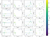 |
Fig. 5. A set of 16 plots showing comparisons of abundances of europium and barium with the isotopic magnesium abundance coloured by Teff. The left eight panels show [24Mg/Fe], [25Mg/Fe], [26Mg/Fe] and the right eight panels show [24Mg/H], [25Mg/H] and [26Mg/H]. |
The comparison of [X/H] with the three magnesium isotopes and europium show a strong correlation (r = 0.795–0.86) that were statistically significant (p < 0.05). The strong correlation between 24Mg and Eu (r = 0.842, p = 0.0087) is consistent with theoretical expectations, as 24Mg is predominantly produced by hydrostatic α capture in massive stars, a process that precedes the r process responsible for Eu production. There appears to be an upper limit in the [Eu/H]–Mg trend, where [Eu/H] stops increasing around ∼0.2 despite continued increase in global Mg and 24Mg. This plateau is less evident for 25Mg and 26Mg. 25Mg and 26Mg also show strong positive correlations with Eu (r = 0.86, p = 0.0061; r = 0.813, p = 0.0141). These isotopes can be produced both by the r process and by the AGB (Karakas & Lattanzio 2003; Vangioni & Olive 2019). However, the uncertainties associated with 25Mg and 26Mg measurements are substantially larger than those for 24Mg, which reduces confidence in the observed correlations.
In contrast to the strong correlations observed with [Eu/H], we find little evidence of correlation between [Mg/H] and [Ba/H]. A moderate correlation can be seen between 24Mg and Ba (r = 0.629, p = 0.095). This is not statistically significant and is unexpected, as Ba and 24Mg are predominantly synthesised in different stellar environments (Karakas & Lattanzio 2003; Vangioni & Olive 2019). However, we see no correlation between Ba and 25Mg and 26Mg, despite expectations that all three are predominantly produced in similar astrophysical environments. This discrepancy may be due to the small sample size, differences in the specific subprocesses within the s process (strong and weak s process (Karakas & Lattanzio 2003; Vangioni & Olive 2019)), or the larger measurement uncertainties associated with the weaker and more blended spectral features of 25Mg and 26Mg. If this result reflects a genuine astrophysical trend, it may suggest that only a small amount of 25Mg and 26Mg is produced during the strong s process.
In Figure 5 we found that the coolest star in the sample ψ Phe, may be an outlier with the most uncertain parameters and so finding good abundances are very difficult. In this case we removed it from the sample to assess how the correlations differ for [X/H]. In every case we find significant increases in the significance levels for all three isotopes with the largest increase being with 25Mg. For all isotopes we find a strong correlation p > 0.75 and r < 0.045. With removal of this outlier we are seeing what we initially expected when comparing to Ba for the heavy isotopes, 25Mg and 26Mg, which is a strong correlation at high significance. This indicates that our results support current theories of nucleosynthetic production sites. For Eu we find that the correlation decreases, where 26Mg is now weakly significant, however 24Mg and 25Mg are still statistically significant.
Direct comparison of [Eu/H] and [Ba/H] against the global [Mg/H] abundance shows a significant correlation. For Mg vs Eu there is a strong positive correlation (r = 0.84, p = 0.009). This suggests that the total Mg is enhanced when Eu is enhanced. Broadly speaking this makes sense because they are both enriched by massive stars and released during Type II Supernovae. Specifically, the largest contributing isotope 24Mg is produced during hydrostatic α-capture in stellar interiors, in a process preceding explosive r process events which Eu is synthesised. For Ba vs. Mg, there is no statistically significant correlation (r = 0.586, p = 0.127). This lack of correlation is expected, as Ba and Mg are primarily produced in different astrophysical environments (Karakas & Lattanzio 2003; Vangioni & Olive 2019). However, some scatter in the data may arise due to galactic chemical evolution (GCE).
Making a comparison to [X/H] may also include effects due to metallicity. To remove any such, the comparisons were repeated with [X/Fe] (see second set of panels in Figure 5). There is some change in how Ba, Eu and Mg interact. A moderate correlation is seen for Mg and Ba (r = 0.618, p = 0.103) and strong significance for Mg and Eu (r = 0.772, p = 0.025). For [Eu/Fe] vs [24Mg/Fe] a strong and statistically significant correlation is seen. For [Eu/Fe] vs [25Mg/Fe] and [26Mg/Fe] we see the same strong correlations (r = 0.849, p = 0.007; r = 0.848, p = 0.007). A second outlier is prominent which weakens the presence of any correlation between Eu and 25Mg. For the comparisons of [Ba/Fe] to Mg and its isotopes, strong correlations are found which are dominated by the two cooler stars. Removal of these data points gives a strong negative correlation in all cases. We can conclude that the [X/Fe] show there is an effect due to metallicity but the final conclusion remains the same, we need more data to be convinced of any real correlations.
4.6. Abundance vs parameters
In Figure 6 we show the relationship between Eu, Ba and Mg against the stellar parameters of Teff and log g. When comparing the neutron capture elements of Ba and Eu to the stellar parameters there is little correlation (r = 0.50, p = 0.20). The same can be said with the Mg to the stellar parameters (Teff: r = −0.03, p = 0.93, log g:r = −0.08, p = 0.86). There is a near significant trend for Ba vs Teff and Ba vs log g. For Ba vs Teff a r = −0.67 and p = 0.066 show a fairly convincing negative correlation with a near significant p-value. This indicates that there may be a correlation but more data is needed to confirm the result. For Ba vs log g a r = −0.65 and p = 0.081 there is also a fairly strong negative correlation with a near significant p-value. These both indicate that higher Teff and lower surface gravity might show more Ba but it is possible that this is an observational or systematic effect. There is no significant correlation between the Ba and Eu abundances which is expected since they are generated in different environments (Vangioni & Olive 2019). There is no correlation between Mg and Teff or log g, suggesting that these abundances are robust to stellar parameter bias. With removal of metallicity bias the same robust results are seen.
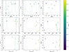 |
Fig. 6. Abundances of europium, barium, and magnesium compared with stellar parameters to examine possible trends coloured by Teff. |
5. Conclusion
We have developed an analysis pipeline for determining magnesium isotopic ratios in stars across a range of spectral types. Validation with reference stars demonstrates good agreement with literature values, confirming the reliability of the method within its effective temperature limits. Our analysis shows that 24Mg consistently dominates the isotopic composition, with 25Mg and 26Mg contributing roughly equal fractions. Examination of individual MgH regions identified Regions 1, 3, 5, 6, 8, 9, and 10 as providing the most reliable isotopic information, while other regions are less sensitive due to limited variation across stars. Elemental abundances of Mg, Eu and Ba are consistent with previous studies, supporting the accuracy of isotopic determinations (Jofré et al. 2015; Hinkel et al. 2014).
Comparison of magnesium isotopes with the r process element Eu and the s process element Ba (Guiglion et al. 2018; Sneden et al. 2014) reveals strong correlations with [Eu/H] but weak or absent correlations with [Ba/H]. A comparison removing outliers resulted in stronger correlations for [Ba/H] with all isotopes. The removal of the outlier resulted in findings that are more consistent with theoretical expectations, as the majority of 24Mg is released by the same process as Eu and 25Mg, and 26Mg are produced through processes releasing s process elements (Vangioni & Olive 2019; Karakas & Lattanzio 2003). With removal of the effect of metallicity similar results were found. The absence of strong dependence on stellar parameters further supports the robustness of the derived abundances and isotopic ratios. Overall, these results validate the reliability of the analysis pipeline and provide a foundation for future studies of magnesium isotopes across diverse stellar populations, contributing to our understanding of chemical evolution in the Galaxy.
Acknowledgments
I would like to thank Kyle Boucher, Peter Cottrell, Michael Elston, Heather Sinclair-Wentworth, and Zachary Lane, for helping me check my arguments. This research has made us of the Python 3 packages, numpy (Harris et al. 2020), pandas (The pandas development team 2020), and matplotlib (Hunter 2007).
References
- Barbuy, B. 1985, A&A, 151, 189 [NASA ADS] [Google Scholar]
- Barbuy, B. 1987, A&A, 172, 251 [NASA ADS] [Google Scholar]
- Blanco-Cuaresma, S., Soubiran, C., Jofré, P., & Heiter, U. 2013, arXiv e-prints [arXiv:1312.4545] [Google Scholar]
- Blanco-Cuaresma, S., Soubiran, C., Heiter, U., & Jofré, P. 2014, A&A, 569, A111 [CrossRef] [EDP Sciences] [Google Scholar]
- Buder, S., Sharma, S., Kos, J., et al. 2021, MNRAS, 506, 150 [NASA ADS] [CrossRef] [Google Scholar]
- Cowan, G. 1998, Statistical Data Analysis (Oxford University Press) [Google Scholar]
- De Bièvre, P., & Barnes, I. L. 1985, Int. J. Mass Spectrom. Ion Processes, 65, 211 [Google Scholar]
- Gay, P. L., & Lambert, D. L. 2000, ApJ, 533, 260 [Google Scholar]
- Gilmore, G., Randich, S., Worley, C. C., et al. 2022, A&A, 666, A120 [NASA ADS] [CrossRef] [EDP Sciences] [Google Scholar]
- Golovin, A., Reffert, S., Just, A., et al. 2023, A&A, 670, A19 [NASA ADS] [CrossRef] [EDP Sciences] [Google Scholar]
- Gray, D. F. 2005, The Observation and Analysis of Stellar Photospheres, 3rd edn. (Cambridge: Cambridge University Press) [Google Scholar]
- Grevesse, N., Asplund, M., & Sauval, A. J. 2007, Space Sci. Rev., 130, 105 [Google Scholar]
- Guiglion, G., Laverny, P. d., Recio-Blanco, A., & Prantzos, N. 2018, A&A, 619, A143 [NASA ADS] [CrossRef] [EDP Sciences] [Google Scholar]
- Harris, C. R., Millman, K. J., Walt, S. J. v. d., et al. 2020, Nature, 585, 357 [NASA ADS] [CrossRef] [Google Scholar]
- Hearnshaw, J. B. 1986, ApSS, 118, 79 [Google Scholar]
- Hearnshaw, J. B., Barnes, S. I., Kershaw, G. M., et al. 2002, Exp. Astron., 13, 59 [Google Scholar]
- Heiter, U., Jofré, P., Gustafsson, B., et al. 2015, A&A, 582, A49 [NASA ADS] [CrossRef] [EDP Sciences] [Google Scholar]
- Heiter, U., Lind, K., Bergemann, M., et al. 2021, A&A, 645, A106 [EDP Sciences] [Google Scholar]
- Hinkel, N. R., Timmes, F. X., Young, P. A., Pagano, M. D., & Turnbull, M. C. 2014, AJ, 148, 54 [NASA ADS] [CrossRef] [Google Scholar]
- Hunter, J. D. 2007, Comput. Sci. Eng., 9, 90 [NASA ADS] [CrossRef] [Google Scholar]
- Iliadis, C. 2007, Nuclear Physics of Stars (Wenheim, Germany: Wiley-VCH Verlag) [Google Scholar]
- Jofré, P., Heiter, U., Soubiran, C., et al. 2015, A&A, 582, A81 [Google Scholar]
- Karakas, A. I., & Lattanzio, J. C. 2003, arXiv e-prints [arXiv:astro-ph/0305011] [Google Scholar]
- Kobayashi, C., Karakas, A. I., & Lugaro, M. 2020, ApJ, 900, 179 [Google Scholar]
- McKenzie, M., Monty, S., Yong, D., et al. 2024a, MNRAS, 534, L35 [Google Scholar]
- McKenzie, M., Yong, D., Karakas, A. I., et al. 2024b, MNRAS, 527, 7940 [Google Scholar]
- McWilliam, A., & Lambert, D. L. 1985, BAAS, 17, 841 [Google Scholar]
- McWilliam, A., & Lambert, D. L. 1988, MNRAS, 230, 573 [NASA ADS] [CrossRef] [Google Scholar]
- Meléndez, J., & Cohen, J. G. 2009, ApJ, 699, 2017 [Google Scholar]
- Pavlenko, Y. V., Harris, G. J., Tennyson, J., et al. 2008, MNRAS, 386, 1338 [NASA ADS] [CrossRef] [Google Scholar]
- Shayesteh, A., Henderson, R. D. E., Le Roy, R. J., & Bernath, P. F. 2007, J. Phys. Chem. A, 111, 12495 [CrossRef] [Google Scholar]
- Sneden, C., Bean, J., Ivans, I., Lucatello, S., & Sobeck, J. 2012, Astrophysics Source Code Library [record ascl:1202.009] [Google Scholar]
- Sneden, C., Lucatello, S., Ram, R. S., Brooke, J. S. A., & Bernath, P. 2014, ApJS, 214, 26 [Google Scholar]
- Soubiran, C., Creevey, O. L., Lagarde, N., et al. 2024, A&A, 682, A145 [NASA ADS] [CrossRef] [EDP Sciences] [Google Scholar]
- The pandas development team 2020, https://doi.org/10.5281/zenodo.3509134 [Google Scholar]
- Thygesen, A. O., Sbordone, L., Ludwig, H.-G., et al. 2016, A&A, 588, A66 [NASA ADS] [CrossRef] [EDP Sciences] [Google Scholar]
- Thygesen, A. O., Kirby, E. N., Gallagher, A. J., et al. 2017, ApJ, 843, 144 [CrossRef] [Google Scholar]
- van Leeuwen, F., de Bruijne, J., Babusiaux, C., et al. 2022, Gaia DR3 documentation, Tech. rep. [Google Scholar]
- Vangioni, E., & Olive, K. A. 2019, MNRAS, 484, 3561 [NASA ADS] [CrossRef] [Google Scholar]
- Yong, D., Lambert, D. L., & Ivans, I. I. 2003, ApJ, 599, 1357 [Google Scholar]
- Yong, D., Lambert, D. L., & Allende Prieto, C. 2004, ApJ, 603, 697 [Google Scholar]
- Yong, D., Aoki, W., & Lambert, D. L. 2006, ApJ, 638, 1018 [Google Scholar]
All Tables
All Figures
|
Fig. 1. Kiel diagram showing the distribution of ISAM stars in temperature space (circled), coloured by metallicity. The background points are the stars from GBS V3 (Soubiran et al. 2024) to show the main sequence more clearly. |
| In the text | |
|
Fig. 2. Individual and combined contributions of Mg isotopes to region 1 of HD 18907. The top left panel shows the synthetic spectral feature from 24Mg only (no contribution from 25Mg or 26Mg). The top right panel shows the feature from 25Mg only, and the bottom left panel shows the 26Mg contribution. The bottom right panel with the fitting region in the blue box, presents the combined synthetic spectrum including all three isotopes, providing the best fit solution for this region. |
| In the text | |
|
Fig. 3. Regions 1 through 10 showing the MgH lines and the fitting region (blue shaded rectangle) for all stars colour coded by effective temperature. Vertical lines mark the positions of the three magnesium isotopes: dot–dash for 24Mg, dashed for 25Mg, and solid for 26Mg. |
| In the text | |
|
Fig. 4. Mean isotopic percentage as a function of region wavelength for 24Mg (red), 25Mg (blue), and 26Mg (green). Error bars indicate the standard deviation of the ISAM for each region. |
| In the text | |
|
Fig. 5. A set of 16 plots showing comparisons of abundances of europium and barium with the isotopic magnesium abundance coloured by Teff. The left eight panels show [24Mg/Fe], [25Mg/Fe], [26Mg/Fe] and the right eight panels show [24Mg/H], [25Mg/H] and [26Mg/H]. |
| In the text | |
|
Fig. 6. Abundances of europium, barium, and magnesium compared with stellar parameters to examine possible trends coloured by Teff. |
| In the text | |
Current usage metrics show cumulative count of Article Views (full-text article views including HTML views, PDF and ePub downloads, according to the available data) and Abstracts Views on Vision4Press platform.
Data correspond to usage on the plateform after 2015. The current usage metrics is available 48-96 hours after online publication and is updated daily on week days.
Initial download of the metrics may take a while.