| Issue |
A&A
Volume 708, April 2026
|
|
|---|---|---|
| Article Number | A381 | |
| Number of page(s) | 14 | |
| Section | Extragalactic astronomy | |
| DOI | https://doi.org/10.1051/0004-6361/202557172 | |
| Published online | 28 April 2026 | |
Multi-wavelength behaviour of the radio galaxy SBS 1343+537: γ-ray flaring activity discovered by Fermi-LAT and coordinated Swift and SRT observations
1
Istituto Nazionale di Fisica Nucleare Roma Tor Vergata, via della Ricerca Scientifica, 00133, Roma, Italy
2
ASI – Space Science Data Center, via del Politecnico, 00133, Roma, Italy
3
Dipartimento di Fisica, Sapienza Università di Roma, P.le A. Moro, 00185, Roma, Italy
4
Università di Trento, via Sommarive 14, 38123, Trento, Italy
5
Dipartimento di Fisica “M. Merlin”, Università e Politecnico di Bari, via Amendola 173, 70126, Bari, Italy
6
Istituto Nazionale di Fisica Nucleare Bari, via Giovanni Amendola 173, 70126, Bari, Italy
7
INAF-Osservatorio Astronomico di Cagliari, via della Scienza, 09047, Cuccuru Angius, Selargius, Italy
8
Space Science Division, Naval Research Laboratory, Washington, DC, 20375, USA
9
Department of Fundamental Physics and IUFFyM, University of Salamanca, Plaza de la Merced S/N, E-37008, Salamanca, Spain
10
ASI – Sardinia Deep Space Antenna, Casa Cantoniera di Pranu Sanguni, 09040, San Basilio, Italy
11
INAF – Istituto di Radio Astronomia, Via P. Gobetti 101, I-40129, Bologna, Italy
12
Istituto Nazionale di Fisica Nucleare Trieste, via Valerio, 34127, Trieste, Italy
13
Università di Roma Tor Vergata, Dipartimento di Fisica, via della Ricerca Scientifica, 00133, Roma, Italy
14
Department of Astronomy, University of Geneva, Chemin Pegasi 51, 1290, Versoix, Switzerland
15
INAF – Osservatorio Astronomico di Roma, viale del Parco Mellini, 00136, Monte Porzio Catone, Italy
★ Corresponding authors: This email address is being protected from spambots. You need JavaScript enabled to view it.
; This email address is being protected from spambots. You need JavaScript enabled to view it.
Received:
9
September
2025
Accepted:
14
February
2026
Abstract
The SBS 1343+537 radio galaxy has a kiloparsec-scale radio jet, and complex kiloparsec-scale morphology. Although its classification is still uncertain, in literature it is indicated as a possible Fanaroff-Riley type I (FR-I) object with extended wings of emission, and core blazar-like properties. It was recently spatially associated with the GeV γ-ray source 4FGL J1346.5+5330, which detected by the Large Area Telescope (LAT), on board the Fermi Gamma-Ray Space Telescope. In June 2024, the Fermi Large Area Telescope (Fermi-LAT) observed enhanced γ-ray activity from SBS 1343+537. The event was followed up by the Neil Gehrels Swift Observatory satellite (Swift) and Sardinia Radio Telescope (SRT) observations. Here, we present multi-frequency data (radio, optical, Ultra Violet (UV), X-ray, and γ-ray) collected during this observing campaign. Our results confirm the detection of a short-lived γ-ray flare, consistent with a power-law spectrum. We report a stable X-ray flux, minor activity in the UV band, and a flux density increase in the radio 20 GHz band, which might indicate a mild spectral index inversion. The broadband spectral energy distribution (SED) modelling confirms a typical blazar-like emission in the core of this source, dominated by one-zone Synchrotron Self-Compton (SSC) and external Compton (EC) leptonic processes.
Key words: astroparticle physics
© The Authors 2026
 Open Access article, published by EDP Sciences, under the terms of the Creative Commons Attribution License (https://creativecommons.org/licenses/by/4.0), which permits unrestricted use, distribution, and reproduction in any medium, provided the original work is properly cited.
This article is published in open access under the Subscribe to Open model. This email address is being protected from spambots. You need JavaScript enabled to view it. to support open access publication.
1. Introduction
Active galactic nuclei (AGNs) are extremely bright core regions of a type of galaxy, where the intense luminosity is powered by the accretion of matter onto the supermassive black hole (SMBH) at the centres of their host galaxies. Through this process, a large amount of energy is emitted across the entire electromagnetic spectrum, from radio waves to γ-rays, outshining the combined light of all the stars in their galaxy, with a large-amplitude variability of the emitted flux over timescales ranging from years to mere minutes (Abdollahi et al. 2024; Padovani et al. 2017). There are two AGNs classes: radio-quiet (∼90%), and radio-loud (∼10%). Radio-loud AGNs, such as radio galaxies, BL Lacertae Objects (BL Lacs), and radio-loud quasars (including blazars), are characterised by powerful radio emission, often associated with relativistic jets extending over kiloparsec-scales. In contrast, radio-quiet AGNs, including Seyfert galaxies and radio-quiet quasars, exhibit much weaker radio output, and the typically lack prominent jet structures (Radcliffe et al. 2021; Peterson 1997; Krolik 1999).
AGNs can also be classified according to their optical and UV spectral properties and the orientation of their relativistic jets with respect to the observer. According to the unified model (Urry & Padovani 1995), the wide variety of observed AGNs types mainly reflects differences in viewing angle and obscuration, rather than intrinsic physical distinctions. When the jet axis is closely aligned with the line of sight, relativistic beaming amplifies the observed emission, producing the class of blazars that includes BL Lac objects and flat-spectrum radio quasars. At larger viewing angles, the boosted emission is reduced and the same systems are observed as radio galaxies, which display extended jet and lobe structures. In addition, AGNs are spectroscopically divided into two categories based on the visibility of their emission-line region: Type-1 and Type-2 AGNs. Type-1 AGNs show both broad and narrow emission lines arising from regions close to the central black hole, while for Type-2 AGNs these broad line regions (BLRs) are hidden by the dusty torus, leaving only narrow lines visible. This orientation-based framework successfully connects quasars, radio galaxies, and blazars as manifestations of the same underlying phenomenon viewed from different directions (Urry & Padovani 1995).
Radio galaxies are often considered to be the parent population of blazars. In the latter the jet aligns closely with our line of sight, while in radio galaxies, the jets are oriented towards a larger viewing angle.
This difference in jet orientation strongly affects the observed emission due to Doppler boosting: jets pointing towards the observer appear significantly brighter and more variable because of bulk relativistic beaming effects, whereas misaligned jets suffer reduced boosting and appear fainter (Urry & Padovani 1995). Radio galaxies have jets and double lobes and are morphologically categorised into two types: FR-I type, in which the peak brightness occurs closer to the core, and Fanaroff-Riley type II (FR-II), in which it is found near the edges of the lobes, in prominent hotspots (Fanaroff & Riley 1974; Chen et al. 2023). FR-I and FR-II radio galaxies also differ in luminosity. In particular, FR-II are brighter than FR-I, and the break value is Lbreak ∼ 1026 W/Hz at 178 MHz (Fanaroff & Riley 1974). FR-I are considered to be the misaligned parent population of BL Lac (Urry et al. 1991).
In addition to their morphological classification (FR-I and FR-II), radio galaxies can also be divided spectroscopically into High Excitation Radio-Galaxies (HERG) and Low Excitation Radio-galaxies (LERG; Hine & Longair 1979) galaxies. This distinction reflects fundamental differences in the accretion mode and host-galaxy environment. HERG are typically powered by radiatively efficient accretion of cold gas, often associated with mergers or cooling flows, producing strong optical emission lines. LERG, on the other hand, are generally radiatively inefficient, fuelled by hot gas from the halo or intracluster medium, and show weak or absent optical lines. In the local Universe, HERG are usually found in younger, star-forming galaxies, while LERG tend to reside in massive, quiescent ellipticals, often in rich environments (Chilufya et al. 2025).
SBS 1343+537 is a radio-loud AGN with the coordinates RA = 206.438980 deg, Dec= + 53.547858 deg (J2000; Petrov & Taylor 2011), and redshift z = 0.1356 (Ahumada et al. 2020), also known as TXS 1344+537, and 4FGL J1346.5+5330 in the Fermi Large Area Telescope Fourth Source Catalog Data Release 4 (4FGL-DR4; Ballet et al. 2024).
The classification of SBS 1343+537 is still considered uncertain. The observed complex radio morphology suggests possible jet reorientation or precession. Radio lobes likely lie near the sky plane, while a precessing jet could explain the blazar variability, and the High Energy (HE) emission (E> 10 GeV) from the so-called, blazar-zone region of the object (Pajdosz-Śmierciak et al. 2022). The total flux density at 144 MHz is above 1.3 Jy, with a luminosity of L ∼ 6.33 × 1025 W/Hz, which is a value at the boundary between FR-I, and FR-II radio galaxies (Pajdosz-Śmierciak et al. 2022). From the Sloan Digital Sky Survey- Data Release 19 (SDSS-DR19)1r-band magnitude (r = 17.01, in the AB magnitude system Oke & Gunn 1983), the radio power, L1.4 ≃ 1.4 × 1025 W Hz−1, places SBS 1343+537 below the Ledlow-Owen dividing line, which is consistent with a FR-I classification (Ledlow & Owen 1996). Jets in some radio galaxies indeed show, indeed, significant deviations from their initial direction, leading to the formation of mirror-symmetric (C-shape) and inversion-symmetric (S- or Z-shape) structures (Rudnick & Owen 1976; O’Dea & Baum 2023).
The kpc-scale radio morphology of SBS 1343+537 is characterised by a double-sided morphology, exhibiting an inversely symmetric geometry (so S-shaped; Sanchez-Saavedra et al. 1990), with a compact radio core, a prominent S-shaped radio jet on both sides, and distinct radio hotspots. Up to 30 kpc from the centre, there is no hotspot in the eastern direction. This rare morphology makes the SBS 1343+537 particularly intriguing for detailed analyses, as extended jets and lobes of this type are rarely observed in high-energy extragalactic sources, and could be produced by non-trivial astrophysical mechanisms. The extended lobes appear to lie close to the plane of the sky, and their configuration may result from a slowly precessing jet (Pajdosz-Śmierciak et al. 2022).
Among the compact radio components in SBS 1343+537, there is a diffuse FR-I-like structure, which is also S-shaped and extends over 370 kpc. These structural elements have been observed by the LOw-Frequency ARray (LOFAR; Shimwell et al. 2017), the Faint Images of the Radio Sky at Twenty-cm (FIRST; Becker et al. 1995), and the Aperitif Data Release 1 (DR1; Pajdosz-Śmierciak et al. 2022). The complex and large-scale morphology of this radio galaxy hosts a blazar-like core, where relativistic jet activity is viewed from a smaller angle of sight (Fig. 1). The National radio astronomy observatory and Very large array Sky Survey (NVSS; Condon et al. 1998) map reveals a slight extension, while high-resolution Very Large Array Sky Survey (VLASS; Lacy et al. 2020; Paliya et al. 2024) data confirm a nodal structure in one of the radio jets. At 54 MHz, the source shows a compact core with extended emission (Pajdosz-Śmierciak et al. 2022).
 |
Fig. 1. (a) Radio properties visible on LOFAR 144 MHz contour radio image of SBS 1343+537 overlaid on the greyscale Faint Images of the Radio Sky at Twenty-cm (FIRST) data. Contours greyscale starts from the 3σ level (0.24, 0.75, 0.66, 0.30, 0.60, 0.85) mJy beam−1. Negative 3σ contours are marked with a dashed line. LOFAR Two-meter Sky Survey (LoTSS) beam of 6 × 6 arcsec is shown in the corner. The red cross shows the reference radio/optical position of SBS 1343+537 (Pajdosz-Śmierciak et al. 2022). (b) Image at 1.359 GHz with visible extended emission by Apertif DR1 at Westerbork Synthesis Radio Telescope (WSRT; Kutkin et al. 2022). Contours start from the 3σ level, with the first positive contour at 0.15 mJy beam−1, and are scaled by a factor of |

On a parsec-scale, the nuclear radio jet of SBS 1343+537 is oriented southeast, aligned with the kiloparsec-scale outflow (Helmboldt et al. 2007), and exhibits a complex structure that may indicate jet reorientation or precession. Such behaviour could also account for the observed blazar-like variability, and HE γ-ray emission (Pajdosz-Śmierciak et al. 2022).
According to Pajdosz-Śmierciak et al. (2022), the study of SBS 1343+537 could help clarify the evolutionary mechanisms of AGN and expand our understanding of the morphological diversity within the blazar population. Consequently, they encouraged multi-wavelength observations and modelling to shed light on physical properties such as the magnetic-field strength and the synchrotron age of their extended structures.
The LAT (Atwood et al. 2009), on board the Fermi Gamma Ray Space Telescope, has detected nearly 4500 AGNs and candidate AGNs (Ajello et al. 2022) emitting in γ-rays, including blazars, radio galaxies (Abdo et al. 2009), and narrow-line Seyfert 1 galaxies (D’Ammando et al. 2015), suggesting the presence of highly relativistic jets in these classes of sources.
On June 23, 2024 (MJD 60484), the Fermi-LAT observed, for the first time, enhanced γ-ray activity from SBS 1343+537 (Ciprini et al. ATel,). Following this Fermi-LAT discovery, multiple Target of Opportunity (ToO) observations were requested of Swift (Gehrels et al. 2004) in the optical, UV and X-ray bands (Giacchino et al. 2024), and of the SRT in the GHz radio band.
Here, we investigated the spectral and temporal behaviour of the beamed emission from the relativistic jet of SBS 1343+537. Specifically, in Section 2 we report the remarkable γ-ray activity by the Fermi-LAT in June, 2024, with data analysis during the flare, together with the ∼17 years of the Fermi-LAT mission survey. In Sections 3 and 4, we describe the analysis of Swift, and SRT data respectively. In Section 5, we describe how we performed a modelling of the radio-to-gamma-ray SED of SBS 1343+537. In Section 6, we summarise our conclusions.
2. Fermi-LAT observations
As reported in ATel#16671, a first outlook of Fermi-LAT to SBS 1343+537 on June 23, 2024 (MJD 60484), yielded an average daily γ-ray flux (E > 100 MeV) of ⟨Φ⟩γ = (2.4±0.9) × 10−7 photons cm−2 s−1 (statistical uncertainty only; Ciprini et al. ATel,). This value is almost 30 times higher than the one in the 4FGL-DR4 catalogue: Φ4FGL ∼ 8 × 10⁻⁹ photons cm−2 s−1. The corresponding photon spectral index was Γ = 2.3 ± 0.3, which is consistent within 1σ with the value in the 4FGL-DR4 of Γ4FGL = 2.678 ± 0.081 (Ballet et al. 2024). These preliminary results were already reported by Casaburo et al. (2025).
2.1. Analysis of Fermi-LAT data
Our Fermi-LAT data analysis was performed using Fermipy v. 2.2.0, an open-source Python framework (Wood et al. 2017), and Fermitools v. 2.2.02, a tool suite for the Fermi-LAT, and Fermi Gamma-ray Burst Monitor (Fermi-GBM; Meegan et al. 2009). We considered two different time intervals. The first focused on ten days between June 20, 2024, and June 30, 2024 (MJD 60481-60491), to include the entire event with the highest γ-ray flux level ever observed from the source, detected by Fermi-LAT on June 23, 2024. The second interval is the full survey of Fermi-LAT from August 04, 2008 at 15:43:37 Coordinated Universal Time (UTC) and to July 06, 2025 at 02:21:59 UTC (MJD 54682.65-60862.10), including the complete period of the Swift and SRT campaigns from optical-to-X-ray, and radio, respectively. The analysis made use of Pass 8 events (Atwood et al. 2013) and all the available photons (front and back) in the [0.1 GeV;300 GeV] energy range. This accounts for the Fermi-LAT energy dispersion effects, by enabling the energy dispersion correction within the binned likelihood framework. This correction3, applied following the Pass 8 Instrumental Response Functions (IRFs), is particularly important below 300 MeV to reduce systematic uncertainties in the spectral fits. In order to reduce the contamination from the Earth limb, cuts on photons arriving with zenith angles of θz > 90 deg for energies of E < 1 GeV, otherwise greater than 105 deg, were applied. The defined Region of Interest (ROI) is 10 deg × 10 deg around our target, with a pixel size of 0.1 deg, and eight evenly spaced logarithmic energy bins. P8R3 SOURCE V3 IRFs were used, along with the Galactic diffuse model gll_iem_v07.fits, and the isotropic diffuse model iso_P8R3SOURCE_V3_v1.txt. The used likelihood spectral fit model includes all sources in the 4FGL-DR4 catalogue located at a maximum distance of 20 deg from the target position. A summary of set parameters is reported in the appendix A. In the spectral analysis, we allowed the isotropic and diffuse backgrounds to vary freely. In addition we allowed spectral parameters of sources within 5 deg of our target to vary freely, and the normalization parameter of all the sources with a test statistic (TS) value TS > 10.
The TS is defined as follows4 (Lehmann & Romano 2006):
![Mathematical equation: $$ \begin{aligned} TS = -2 \log \left( \frac{\mathcal{L} _{\max ,0}}{\mathcal{L} _{\max ,1}} \right) = 2 \left[ \log \mathcal{L} _{\max ,1} - \log \mathcal{L} _{\max ,0} \right] \end{aligned} $$](/articles/aa/full_html/2026/04/aa57172-25/aa57172-25-eq2.gif) (1)
(1)
where ℒmax, 0 is the maximum likelihood value for the null hypothesis H0 (i.e. the background-only model without the source), and ℒmax, 1 is the maximum likelihood value for the alternative hypothesis H1 (i.e. the model including the source).
Given that extended-source modelling in Fermi-LAT data is typically only considered for angular extensions greater than 0.05 deg, and that the target source SBS 1343+537 has a measured extension of only 0.006 deg (Jarrett et al. 2000), considering this as a point-like source in the analysis is justified.
In Fig. 2, the SEDs of the two periods are reported applying a TS condition to set upper limits (ULs). Results clearly indicate that the flux during the flaring event is significantly greater than the one derived from all Fermi-LAT observations, highlighting a noteworthy increase in activity. We also notice a cut-off at E ∼ 104 MeV.
 |
Fig. 2. SED fits of SBS 1343+537 using log parabola, and power-law functions, for the flaring event (blue) and Fermi-LAT full period (green). The UL is reported when TS < 4. |
Both the γ-ray SED curves were fitted using a power law and a log-parabola model.
The power-law function is given by Abdollahi et al. (2023):
 (2)
(2)
where N0 is the normalisation factor, Γ is the spectral index, and Eb is the energy scale.
The log-parabola function is given by Abdollahi et al. (2023):
 (3)
(3)
where Φ0 is the flux density at E0, α is the slope index, β is the curvature, and E0 is the scale parameter.
The scale parameter of the power law, resulting from the analysis is Eb ∼ 620.848 MeV, which is in agreement with the value reported in the 4FGL-DR4 catalogue (Ballet et al. 2024), and it has been used as scale parameter E0 for the log-parabola fitting. The fitting results are summarised in Table 1. This table shows the variation in spectral states derived from the analysis of the two periods, and compares the power-law indexes, and log-parabola spectral parameters with the corresponding values listed in 4FGL-DR4. During the flare period, the photon index, Γ, decreased to 2.368 ± 0.023, compared to 2.678 ± 0.081 reported in the 4FGL-DR4 (Ballet et al. 2024), suggesting a harder spectrum. Similarly, the α parameter of the log-parabola model fit also decreased, while the β remained largely consistent across both periods and close to zero, confirming the minimal curvature in the spectral shape. The comparison between the spectral parameters from the ∼17-year survey and those reported in the 4FGL-DR4 catalogue shows agreement within 2σ, supporting the stability of the γ-ray spectrum outside the flaring states.
Averaged spectral parameters for the two periods (flare event, and Fermi-LAT full period).
According to Abdollahi et al. (2022), the γ-ray sources are modelled with a curved spectral form if the TS satisfies the following condition:
![Mathematical equation: $$ \begin{aligned} TS_{\rm curv} = 2\left[\log {\mathcal{L} _{\rm curv}}-\log {\mathcal{L} _{\rm PL}}\right]>4 \end{aligned} $$](/articles/aa/full_html/2026/04/aa57172-25/aa57172-25-eq7.gif) (4)
(4)
which corresponds to a Confidence Level (CL) value of 2σ. Here ℒcurv and ℒPL are the likelihood values obtained by fitting the source spectrum with a curved model and a simple power law, respectively. In our analysis, we used a log-parabola model for the curved spectrum. The comparison between the power-law and log parabola models is possible because they are both nested models. Results for both periods exhibit a TScurv value of ∼0, indicating that the log-parabola model is not preferred over the power law model, which is consistent with the results reported in the 4FGL-DR4 catalogue (Ballet et al. 2024). The energy flux (E> 100 MeV), obtained by the spectral fitting, is given in Table 2. As anticipated in the quicklook analysis of ATel#16671 (Ciprini et al. ATel,), the flux increase is more than one order of magnitude.
Energy flux, in the 100 MeV to 300 GeV range obtained by spectral fitting.
In Fig. 3, we show the light curve for the full ∼17 years of Fermi-LAT observations. Because of the weakness of the source, we had to apply the adaptive binning method, with starting bins of 90 days (Lott et al. 2012)5. This procedure was critical as it dynamically adjusted bin sizes to optimise the significance of the detection. It is possible to have a higher temporal resolution during intense flux states, while preserving statistical reliability during fainter, quiet, epochs. The flare period was really very short and it is represented by the thin red line in Fig. 3. Then, even if the flux was ∼3.5 × 10⁻¹¹ erg cm−2 s−1 (Table 2) during the considered flare period, when applying the adaptive binning the broader points do not see the flux of the flare period. Consequently, the flaring period does not correspond to the peak of activity of the source during the full period observed by Fermi-LAT. The apparent flux enhancements (‘bumps’) visible in the light curve are produced by the adaptive binning procedure and limited photon statistics.
 |
Fig. 3. γ-ray (E> 100 MeV) flux light curve of SBS 1343+537 during the full period of Fermi-LAT. The red line highlights the flare period. Each bin size was adjusted to ensure a minimum significance of TS ≥ 10. |
We performed a flux variability analysis using the data from the light curve to investigate the temporal behaviour of the source, and assess its level of variability over the full Fermi-LAT observation period. The flux variability was calculated as a normalised excess variance (Nandra et al. 1997; Abdo et al. 2010b,a; Schleicher et al. 2019):
 (5)
(5)
where σ2 is the variance of the flux, ⟨δ2⟩ is the mean squared uncertainty of the flux, and ⟨F⟩ is the mean flux. This method allowed us to measure the intrinsic variability of the source while accounting for measurement uncertainties, providing valuable insight into the source’s dynamic activity during the full observational period. The mean flux was found to be ⟨F⟩ = 3.88 × 10⁻¹² erg cm−2 s−1, with a variance of 2.18 × 10⁻¹⁴ erg2 cm−4 s−2. These values yielded a flux variability fraction of Fvar = 0.13, indicating a non-negligible, but small, level of intrinsic γ-ray variability of SBS 1343+537.
In addition to the overall flux variability, to quantify the temporal variations of the flux, we computed the slope, k, between each pair of subsequent time-series data points (i.e. the rate of change in flux), considering the entire Fermi-LAT observation period:
 (6)
(6)
where △F is the variation in flux between two consecutive observations, and △t is the corresponding time interval. This allowed us to provide a more detailed insight into the temporal rate of change of the flux (Fig. 4). The corresponding time values were taken as the midpoints between adjacent time bins, reflecting the average time over which each slope was evaluated.
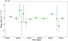 |
Fig. 4. Flux variability analysis of SBS 1343+537, showing rate of change of the γ-ray flux (slope) as a function of mid-time for each time interval. The plot illustrates variations in flux, with error bars representing the uncertainty in the slope and time. |
Due to the weakness of the source it was not possible to perform an analysis of the daily spectral variability in relation to the flux.
We also searched for HE photon emission, with energies exceeding 10 GeV emitted by SBS 1343+537. To assess the likelihood that these photons originated from our source, we used the gtsrcprob tool6 to compute the association probability for each HE photon. Then, we selected events with a source-association probability greater than 95%, resulting in a sample of 11 photons (Table 3).
HE photons with energies of E > 10 GeV.
Three of these HE photons were detected on May 22, 2024 (MJD 60452.3), June 8, 2024 (MJD 60469.0), and June 22, 2024 (MJD 60483.6), respectively: i.e. in the days immediately preceding the large flare. In particular, the highest energy event among them (photon energy of 21.17 GeV) was detected the day before. This could support a harder-when brighter trend during the flare.
3. XRT and UVOT observations
After the powerful γ-ray activity of SBS 1343+537, observed on June 23, 2024 (MJD 60484) by Fermi-LAT, we requested two ToO observations of Swift on June 24 (MJD 60485) and July 10, 2024 (MJD 60501). The source was observed by Swift on 2024 June 25 (MJD 60486), and 29 (MJD 60490), and on July 8 (MJD 60499), 10 (MJD 60501), 12 (MJD 60503), and 16 (MJD 60507).
The Swift/X-Ray Telescope (XRT) data (Burrows et al. 2005) were acquired in photon counting mode, while UltraVio let/OpticalTelescope (UVOT) data (Roming et al. 2005) were acquired in imaging mode. The first observation was carried out in four photometric filters, and the remaining five observations in all six optical/UV photometric filters: i.e. the optical U, V and B, and the UV W1, W2 and M2 whose central wavelength ranges from 1928 Å to 5468 Å (Poole et al. 2008). Then, we reduced the data taken by the Swift/XRT and the Swift/UVOT instruments during the six observations. The exposure times are given in Table B.1. Notice that UVOT data were not available for July 12, 2024 (MJD 60503). The XRT data analysis was performed using the ASI-Space Science Data Center (ASI-SSDC) XRT interactive analysis tool7 developed by the ASI-SSDC team8. In turn, this interactive tool executes the xrtpipeline v. 3.7.09 and various other tasks for data reduction, all included in XRTDAS v. 3.7.0 software package developed by ASI-SSDC and released by NASA High Energy Astrophysics Archive Research Center (NASA-HEASARC)10 within the HeaSoft v. 6.31.1 package and the XSPEC v. 12.13.1e package (Arnaud 1996) for the spectral analysis (also included in the HEASoft package). The latter was performed in the [0.4 keV−10 keV] Swift/XRT range, with a binning of eight intervals. The XSPEC uses a phabs*powerlaw model to fit the spectrum. In this model, phabs includes the Galactic line-of-sight absorption. The hydrogen column density was fixed to NH = 1.19 × 1020 cm−2 (HI4PI Collaboration 2016). X-ray fluxes were extracted in the soft [0.4 keV−2 keV], hard [keV−10 keV] and full [0.4 keV−10 keV] bands. The temporal evolution of the X-ray flux for all the three considered energy bands is given in Fig. 5. From this plot, we notice that the hard, and soft X-ray components exhibit a similar trend, with the hard flux being consistently higher than the soft. We observed that the hard-to-soft flux ratio exhibits relative stability, indicating no significant spectral evolution. The overall trend in the emission also suggests a stable pattern. The stability in the X-ray band is confirmed by considering the quantity (Taylor 1997):
 (7)
(7)
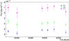 |
Fig. 5. X-ray-flux light curves of SBS 1343+537 from XRT data in the soft (blue), hard (green) and full (magenta) energy bands. |
As results we obtain Nσ < 1 for the three bands (i.e. data are compatible at a 1σ uncertainty level).
The UVOT data analysis was performed executing the ASI-SSDC UVOT archival images analysis pipeline (initially developed from 2006–2007), based on the official UVOT software included in the HEASoft package (version 6.26.1)11. A source position estimation was executed to verify and improve the source centroid with respect to the Swift attitude. The source aperture photometry was run to extract source counts in a standard aperture (5″ radius), and the background in annular aperture with radii of 26″ and 35″, then converting the extracted magnitude to de-reddened optical/UV flux densities through the application of conversion factors included in the CALibration 390 DataBase (CALDB; Poole et al. 2008). An extinction E(B-V) value of 0.0094 (Schlafly & Finkbeiner 2011) was applied for de-reddening together with a mean interstellar extinction law (Fitzpatrick 1999).
In Fig. 6, we report the UVOT light curves for each photometric filter. Similarly to the XRT data, we checked if UVOT data show variability, considering the number of σ (Eq. (7)). We obtain Nσ < 3 for the B, U, M2 and V bands; while we obtain Nσ > 3 only for the W1 and W2 filters, respectively Nσ = 3.53 and Nσ = 3.05, which indicate a possible variability near the significance minimal threshold.
 |
Fig. 6. Optical and UV flux light curves of SBS 1343+537 from UVOT data using the V (blue), B (green), U (magenta), W1 (orange), M2 (red) and W2 (yellow) photometric filters. |
4. SRT observations
4.1. SRT ToO observations
We requested a ToO on SBS 1343+537 with the SRT 64 m (Prandoni et al. 2017) on July 15, 2024 (MJD 60506), at 4.8 GHz and 20.6 GHz. Then, we carried out seve additional observing sessions, up to September 12, 2024 (MJD 60565) of 2.5 hours each on a weekly cadence in order to follow the evolution of the radio flux density at GHz(cm) frequencies and the spectral index. The observations with the C-low receiver (4.8 GHz) were performed with the total-power backend, with the Local Oscillator (LO) of 4600 MHz and a bandwidth of 250 MHz, which corresponds to the cleanest band of the receiver, while the observations with the K-band receiver were carried out with Sardara (Melis et al. 2018) using the LO of 19 900 MHz, an effective bandwidth of 1250 MHz and 1024 channels. For both frequencies, we alternated On-The-Flight (OTF) cross-scans centred on the target and on the flux of the two radio galaxies, 3C 286, and 3C 295, which were used as calibrators and were located at a similar azimuthal elevation at the time of the observations.
4.2. SRT regular observations
A preliminary analysis of the SRT ToO observations, seemed to indicate a flaring activity of the source, likely linked to the γ-ray activity observed by Fermi-LAT on June 23, 2024 (MJD 60484). Consequently, in December, 2024, we proposed to carry out a regular, bi-weekly, monitoring with the SRT, during the first semester of 2025. The aim of these observations was to complete the study of the single-dish flux variability in the radio band, in terms of flux density and spectral index. The proposal was accepted granting a total of 13 epochs of 2.5 h per session from January 30, 2025 (MJD 60705) to June 20, 2025 (MJD 60846).
4.3. Analysis of SRT data
A data analysis was performed with the single-dish imager (SDI) software. This tool is designed to perform continuum and spectropolarimetric imaging, optimised for OTF scan mapping and suitable for all SRT receivers/backends (Egron et al. 2017b,a; Marongiu et al. 2020). The calibration procedure included the corrections for the frequency-dependent gain curves, plus compensations for the pointing offset measured on each scan. Additional opacity and atmospheric corrections were added in the case of K-band data. Through the shape of the cross-scans, which have a Gaussian shape and a width consistent with the beam width both at 4.8 GHz and 20.6 GHz, we were able to verify that the source is point-like at both frequencies. Considering the extreme source size at 150 MHz with very prominent wings larger than the beam size at 20.6 GHz, we conclude that the emission associated with the extended regions is negligible compared to the emission from the core in the K band. At 4.8 GHz, the beam size is larger than the total angular extent of the source reported in the literature; therefore, possible extended emission cannot be resolved and may still contribute to the total flux density. Given the sensitivity of SRT at 20.6 GHz, however, this contribution may be negligible as well. A detailed separation of compact and extended components would require dedicated high-resolution observations and a significantly more in-depth analysis, which is beyond the scope of the present work. In the following, we therefore consider the total flux density and account for any possible contribution from extended emission in the interpretation of the results. The SRT Half-Power Beam 460 Width (HPBW), corresponding to the Full Width at Half Maximum (FWHM) of the antenna beam, is approximately 3.8′−3.9′ at 4.8 GHz and 0.9′−1.0′ at 20.6 GHz.
The resulting light curve and evolution of the spectral index α (with Sν ∝ να) are presented in Figure 7, and the associated data are provided in Table C.1. Additional opacity and atmospheric corrections were added in the case of K-band data. Following the method described in Giroletti & Righini (2020), the flux density is measured by fitting a Gaussian profile to a number of cross-scans. Considering the width of the Gaussian profiles, which is consistent with the beam width both at 4.8 GHz and 20.6 GHz, we were able to verify that the source is point-like at both frequencies. Note that it was not possible to observe in the K band on September 12, 2024 (MJD 60565) and on April 22 (MJD 6078), May 10 (MJD 60805), and June 20, 2025 (MJD 60846) due to the rainy conditions. Additionally, the measurements in the C band on January 30 (MJD 60705) and March 25, 2025 (MJD 60759) were discarded due to high Radio Frequency Interference (RFI).
 |
Fig. 7. Upper panel: Radio light curve of SBS 1343+537 obtained at 4.8 GHz and 20.6 GHz with SRT, from July 15, 2024 (MJD 60506) to June 20, 2025 (MJD 60846). Lower panel: Evolution of the spectral index α of SBS 1343+537. |
In the literature, few observations can be found for SBS 1343+537 at radio frequencies. The source is reported to have a flux density of ∼420 mJy at 1.4 GHz from the NVSS survey (White & Becker 1992; Condon et al. 1998) which, with its ∼45″ beam, includes both compact and extended emission components. At 4.85 GHz, a flux density of ∼240 mJy was measured in the Green Bank 6 cm (GB6) survey, obtained with a larger, ∼3.5′, beam that also encompasses possible diffuse emission (Gregory & Condon 1991). Inspecting data from Table C.1, we notice that, at 4.8 GHz, they are consistent, within the error bars, with a constant, weighted, average flux density of (244±2) mJy. Archival radio flux densities retrieved from the NASA Extragalactic Database (NED) database (Chen et al. 2022) were used to construct the broadband SED, including data points at 4850 MHz, 1400 MHz, 365 MHz, 74 MHz, and 34 MHz, obtained with different instruments and at different epochs. Keeping in mind the difficulty in drawing conclusions from an SED constructed using data points obtained in different epochs and in different observing modes, we want nevertheless to highlight some interesting features. Firstly, the historical and SRT 4.85 GHz data have very similar values. Considering the very small variability shown by our observations on timescales of months, this might indicate that the source, at this frequency, has a nearly constant flux density, on both short and long timescales. Also the historical measurements at 1.4 GHz, which span a time interval of more than 20 years, seem to show very mild (close to none) variability. Lastly, the archival 4850 MHz, 1400 MHz, 365 MHz, 74 MHz, and 34 MHz, data points appear aligned along a power-law model with slope, estimated by the fit, −0.5755 ± 0.0087. For comparison, we also fitted the flare data and obtained a slope of −0.023 ± 0.017 (Fig. 8a).
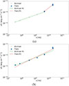 |
Fig. 8. Fit to the archival and flare radio SEDs. (a) Comparison between flare data and archival low-frequency ones. (b) Comparison between radio data using archival low-frequency ones and archival or flare data at frequencies between 4.8 GHz and 22 GHz. |
The points reported above regarding the archival data could indicate that the flux density at 20.6 GHz is affected by significant variability, which mostly dissipated before arriving at 5 GHz; this shows a spectral evolution similar to the one displayed by several blazars including the type 4 sources reported by Angelakis et al. (2012). Note that these sources are described by the authors as showing a steady, steep, low-frequency spectrum consistent with a power-law model with a slope (e.g., ∼0.5), similar to the one we find for the historical SED of SBS 1343+537. We also compared the radio data using the low-frequency ones and archival and flare data at frequencies between 4.8 GHz and 22 GHz. The fit results are α = 0.505 ± 0.039 and α = 0.416 ± 0.037, respectively for archival and flare data, showing the harder spectrum in the last case. At 20.6 GHz, our SRT observations show an increase of the flux density of approximately 14% within 40 days, from July 15 (MJD 60506.9) to August 22, 2024 (MJD 60544.8), when it reaches its peak. After this date, the measured 20.6 GHz flux density starts decreasing, suggesting a possible inversion of the spectral index observable since September 06, 2024 (MJD 60559.8); this is shown in the lower panel of Fig. 7. Since the emission from extended regions would contribute a constant value to the 5 GHz flux densities measured with SRT, isolating the emission from the central region would shift the spectral index towards more inverted values; however, the modulation of the spectral index shown in Fig. 7 (lower panel) would be the same. New measurements from regular observations acquired since January 30, 2025 (MJD 60705) show that the K band flux density persisted in its decreasing trend until March 10, 2025 (MJD 60744), confirming that we effectively sampled a flare with excellent precision (with an uncertainty of just a few days). These new data seem to confirm a spectral trend consistent with the evolution of the flare in the K band, showing a marked steepening of the spectrum after the initial hardening. The fact that only one flare has been observed in the K band during 2024 and 2025, and that it closely follows the γ-ray event, supports the hypothesis that the radio flare is associated with the γ-ray one. On the other hand, in the C band (4.8 GHz), there is no significant trace of variability. This is likely due to the energy dissipation of the flare before reaching lower radio frequencies or to the synchrotron self-absorption that has more significant effects at lower radio frequencies.
5. Multi-frequency SED
The estimated fluxes in the radio, UV, X-ray, and γ-ray bands from the flare observed in June 2024, along with archival data were used to build the full-band SED. Archival data were retrieved through the SED-builder tool12 hosted at the ASI-SSDC. This tool allows the users to search data in the catalogues, as for example the NED and the 4FGL-DR3 (Abdollahi et al. 2022), and to list their own data. In our case, archival multi-frequency data date back to the early 1990s. The archival SED data (grey data points) and those of the June 2024 flare (blue data points) are compared in Fig. 9.
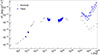 |
Fig. 9. Full band SED of SBS 1343+537 built using multi-epoch past archives (grey data points) dating back the 1990s, and the June 2024 flare epoch (blue data points). The references corresponding to each archival data point are available within the NED database from which the archival SED was generated. |
We notice that the radio, UV, and X-ray data collected by our ToO and multi-frequency observing campaign after the γ-ray flare, are still compatible with archival data. In contrast, the γ-ray data from the flare epoch are about one to two orders of magnitude higher than the archival ones, possibly indicating shock-energised jet components, knots and blobs, magnetic-field increase, and particle acceleration processes, as well as possible increase of the bulk relativistic beaming.
The broadband multi-frequency SED of SBS 1343+537 (both the archival non-simultaneous data and the simultaneous Fermi-LAT, Swift/XRT, Swift/UVOT, and SRT data from our multi-frequency observing campaign shown in Fig. 9) were modelled using the JetSet v. 1.3.1 tool (Tramacere et al. 2009, 2011; Tramacere 2020). This is an open-source framework written in C/Python, designed to simulate the radiative and acceleration processes occurring in beamed relativistic jets of extragalactic, and Galactic objects, and also in unbeamed objects, enabling the fitting of SEDs data to numerical models. This tool includes radiative processes, such as SSC, and the interaction between the former and the Cosmic Microwave Background (CMB). The broadband SED is modelled with a single-zone (blob) leptonic mechanism, where the low-energy emission component arises from synchrotron radiation produced by a population of freshly accelerated electrons, and the HE emission component is predominantly generated through SSC and EC processes. The jet has conical geometry, with a semi-opening angle, θopen. The emitting blob has a spherical geometry with a radius of R, a tangled magnetic field of B; it is moving with a bulk relativistic Lorentz factor, Γ, along the jet axis, with a viewing angle of θ with respect to the line of sight. The radius, R, of the blob is implemented as a functionally dependent parameter in JetSet:
 (8)
(8)
where RH is the distance from the SMBH, and θopen is the jet opening angle.
The electron population is characterised by a broken power-law energy distribution, depending on the Lorentz factor, according to:
 (9)
(9)
where γmin, γbreak, and γmax are, respectively, the minimum, break, and maximum Lorentz factors, p1 is the spectral index below the break; p is the spectral index above the break, and N is the number density of the emitters. The normalisation factor, K, is such that:
 (10)
(10)
In addition to the SSC emission, we also took into account the presence of external radiative fields emitted by the dusty torus (DT), the BLR, and an accretion disc contributing to the EC channel.
The disc was modelled as a single temperature blackbody, with the disc luminosity LDisc, and temperature, TDisc, treated as free parameters during the fitting process of the archival data. The resulting values were set to fit the flare ones.
The radii of the BLR and DT were determined based on the disc luminosity according to Kaspi et al. (2007) and Cleary et al. (2007) and were implemented as functionally dependent parameters in JetSet:
 (11)
(11)
 (12)
(12)
 (13)
(13)
The covering factors of the DT and BLR were fixed to the standard τDT = 0.1 and τBLR = 0.1 (Smith 1981; Ghisellini & Tavecchio 2015). Following the approach of Otero-Santos et al. (2025), we also took into account a component to model the extended jet radio emission, that is, the emission below the synchrotron self-absorption (SSA) frequency of the blob. This emission was modelled as a power law with an index of αradio starting from the frequency  and with an exponential cut-off at
  . This represents an extended jet scenario, where the spectral window between
  and
and  reflects the integrated optically thin synchrotron radiation emitted by successive layers of aged electrons, whose distance from the central blazar zone increases with cooling time. The lower frequency segment, below
  , captures the portion where synchrotron self-absorption dominates. Although this component is constructed from a phenomenological standpoint, the derived value of
  may still offer insights into the magnetic-field configuration, particularly under assumptions such as that of a conical jet geometry. The
  based on the two radio data points with the lowest frequencies at
  and
and  was fixed at 107 Hz, that is, without loss of generality, below the lowest frequency radio data points. We thus left the cut frequency
  as a free parameter to model the archival data. The resulting value was set to model the flare data.
We then performed a model fitting using the JetSet ModelMinimizer module with an iminuit minimisation (Dembinski et al. 2020). The fits are shown in Fig. 10a (archival data) and Fig. 10b (flare data). Due to the lack of flare data in the millimeter-to-optical frequency range, available archival data (∼1011 Hz to ∼1012 Hz) were used to constrain the model within this spectral window. The resulting parameters describing each model are reported in Table D.1. Notice that, for the modelling with JetSet, flux densities at same frequencies were averaged to reduce redundancy and improve the stability of the fit.
 |
Fig. 10. SEDs of SBS 1343+537 modelled by JetSet. (a) Archival data, non-simultaneous SED data, and data-model residuals. (b) The flare-epoch (our multi-frequency campaign) using Fermi-LAT, Swift/XRT, Swift/UVOT, SRT data, and data-model residuals is shown. |
Both the two SEDs exhibit the double-bump shape, indicating non-thermal processes in the relativistic jet. This shape is consistent with a dominant blazar zone responsible for the HE emission of SBS 1343+537.
A quantitative comparison between the archival and flaring SEDs allowed us to explicitly characterise the evolution of both the synchrotron and the dominant inverse Compton (IC) components. During the flaring state, the synchrotron peak frequency shifts from log10(νsyn) = 13.36 − 13.60 Hz, corresponding to Δlog10ν ≃ 0.24 (a factor of ≃1.75), while the synchrotron peak flux increases from log10(νFν) = − 11.83 erg cm−2 s−1 to –11.75 erg cm−2 s−1, i.e. by Δlog10(νFν)≃0.09 (a factor of ≃1.2). In the HE band, the IC emission is dominated by EC scattering off DT photons (ECDT). The ECDT peak frequency shifts from log10(νEC, DT) = 21.27 − 21.58 Hz, corresponding to Δlog10ν ≃ 0.30 (a factor of ≃2.0), while the corresponding peak flux increases from log10(νFν) = − 11.08 erg cm−2 s−1 to –10.68 erg cm−2 s−1, i.e. by Δlog10(νFν)≃0.40 (a factor of ≃2.5). This suggests that the flare cannot be explained by changes in Doppler beaming alone, nor by variations in the magnetic field alone. For the synchrotron emission, we obtain asyn ≃ 0.35, which is well below both expectations, indicating that the flare cannot be explained by a pure beaming-driven scenario. The fact that the flaring state is best explained by variations of multiple physical parameters is further supported by the differences observed between the best-fit model parameters describing the archival and flaring SEDs.
At low frequencies (from radio to UV), we notice the synchrotron radiation component (dashed magenta line) due to the relativistic electrons moving in the magnetic field of the jet. At these frequencies, the peak is placed at approximately 1014–1015 Hz, making this an intermediate-peaked blazar, overwhelmed by the thermal emission from the host galaxy (dashed orange line). Regarding the radio zone, the radio fit accounting for flare data (Fig. 10b) is steeper than archival ones (10a). It can be because the extended structure is not fully taken into account because of the lack of lower frequency radio data regarding the flare period. The host galaxy contribution, dominant from Infra-Red (IR) to optical bands, was modelled as a blackbody emission, highlighting the role of the massive elliptical galaxy hosting the AGN in SBS 1343+537.
At higher energies, we modelled a dominant EC component, involving seed photons from external sources such as the DT, the BLR, and the accretion disk. These seed photons for the IC scattering contribute to the observed high γ-ray energy SED on June 23, 2024 (MJD 60484), suggesting that interactions between the jet and the surrounding photon fields play a crucial role in the flare activity of this peculiar FR-I radio galaxy with a dominant blazar-zone at high energies. These external photon populations introduce distinct subcomponents in the model, in particular in the soft X-ray to γ-ray range, indicating that multiple seed photon populations can contribute to the IC emission. The synchrotron component is also enhanced in the flaring state, implying a higher energy injection in the electron population, likely due to an increase in acceleration efficiency or a change in the jet’s physical conditions, which occur in the jet-shock scenario. Sudden and transient changes in the jet’s physical conditions (increased energisation of electrons, bulk Doppler boosting, or magnetic- field intensity) are the most likely, rather than a long-term evolution of the thermal seed components.
Comparing the two states, the flaring episode is characterised by enhanced emission and spectral shifts, particularly in the γ-ray domain, with a more substantial role for EC mechanisms, likely involving both the DT and the BLR. Such flaring activity discovered by the Fermi-LAT is therefore driven by increased efficiency in the interaction with the external radiation fields, beyond particle acceleration.
Lastly, by defining the magnetic-energy density  , and the electron energy density ue:
 (14)
(14)
where mec2 is the rest energy of the electron, and using the parameters of the flare period from Table D.1, we computed the ratio between the magnetic-energy density, and the electron one (Singh et al. 2020), resulting in uB/ue ≃ 0.4, and pointing to a particle-dominated radiative emission.
6. Conclusions
The SBS 1343+537 is a radio-loud AGN that exhibits an intriguing FR-I radio morphology alongside likely prominent blazar features. It stands out as one of the closest sources identified in recent LOw-Frequency ARray (LOFAR) observations of seven blazar candidates with rare radio morphologies (Pajdosz-Śmierciak et al. 2022). This object is characterised by two-sided jets embedded within a multi-directional, extended, lobe-like structure. In particular, its radio-band geometry displays an inversely symmetrical S-shaped morphology (Battaner et al. 1990).
The peculiar S-shaped radio jet morphology of SBS 1343+537 can be caused by Magneto Hydro Dynamics (MHD) instabilities or jet precession, and can accrete disturbances or shocks, which propagate within its structured jet and lead to this discovered γ-ray flare on June 23, 2024. On this day, the Fermi-LAT observed enhanced γ-ray flux ∼30 times higher than the one reported in the 4FGL-DR4 catalogue (Abdollahi et al. 2022) from SBS 1343+537. We then performed a dedicated multi-wavelength observing campaigns, and analysed Fermi-LAT, Swift (UVOT, and XRT), SRT data.
In the Fermi-LAT analysis, we considered the flare period and the full ∼17-year period up to July 06, 2025. The comparison of the flaring-state SED with the SED built on the entire Fermi-LAT all-sky survey period clearly show the higher flux, with the flare SED consistent with a power-law model and no curvature. This is in agreement with what was reported in the 4FGL-DR4 catalogue (Ballet et al. 2024). The light curve shows that the flaring event was concentrated within a short time interval of a few days, while the flux variability has low level of fluctuations with a variability fraction of Fvar = 0.13. A possible hardening during the flare activity is corroborated by the emission of three HE photons (E> 10 GeV) during the days before the observed peak of the flaring activity.
X-ray observations in the soft, hard, and full bands, show similar trends with the hard flux being consistently higher, and no significant spectral evolution occurring. The UVOT observations in six photometric filters (V, B, U, W1, M2, and W2) are characterised by no variability except for the W1 and W2 bands.
The SRT radio data point out an approximately constant weighted average flux density of (242±2) mJy at 4.8 GHz. The comparison with historical data, between 34 MHz and 4.85 GHz, also suggest minimal variability on longer timescales, and a steep radio spectrum at low radio frequencies. In contrast, at 20.6 GHz a flux density increase from (206±12) mJy to (256±13) mJy was observed within a 40-day period (from July 15 (MJD 60506.9) to August 22, 2024 (MJD 60544.8)), followed by a decrease, suggesting a possible radio-spectral index inversion. This behaviour suggests a potential flaring activity propagating from higher radio frequencies, possibly connected to the γ-ray flare, as confirmed by further SRT observations performed from January 30, 2025 (MJD 60705), to June 20, 2025 (MJD 60846).
Flaring and archival SED data were modelled with one-zone SSC, and EC leptonic model mechanisms (the latter due to DT and BLR), characterising the dominant blazar-like nature of the source. The contribution of the host-galaxy at a frequency ∼1014 Hz to 1015 Hz is also evident. This unique γ-ray flare in June, 2024 of SBS 1343+537 suggests a more efficient particle-acceleration process during this epoch, which is possibly linked to changes in the jet’s magnetic field or the injection of fresh energetic electrons.
Objects such as SBS 1343+537 could be of some interest for Ultra High Energy (UHE) neutrinos, as analyses of IceCube (Aartsen et al. 2017) data widely suggest that the candidate for the bulk of extragalactic PeV neutrino emissions is a population of radio galaxies. FR-I radio galaxies are good candidates (Murase & Waxman 2016), especially during sporadic but intense γ-ray flares, as this discovered by the Fermi-LAT in SBS 1343+537.
Finally, while intriguing, our Fermi-LAT data, and the other radio, UV, and X-ray flux data collected during our multi-frequency observing campaign dedicated to this stand-alone γ-ray flare of SBS 1343+537, do not allow us to propose any precession hypothesis on the intrinsic origin of this S-configuration in the radio maps. Jet precession, nutation, and wobbling can enhance jet curvature and brightness (Graham et al. 2015) and may be related to a possible central, gravitationally bound system of a binary SMBHs. The binary SMBH scenario has been proposed, for example, for a bright Very High Energy (VHE) γ-ray BL Lac object monitored by Fermi-LAT and based on a periodicity analysis (Abdollahi et al. 2024). Similar morphologies are observed in several S-shaped radio galaxies, such as PKS 2300–18, whose jet precession or reorientation has been interpreted as evidence of binary SMBH systems (Misra et al. 2024).
While we do not aim to provide a conclusive result on jet-precession-model or AGN evolution, our observation of a clear radio flare at 20 GHz (temporally associated with γ-ray activity) and the absence of variability at a lower radio frequency (5 GHz) can be consistent with a scenario in which the emission originates in compact regions of the jet, and dissipates before propagating to larger scales. Future observations of SBS 1343+537 will be important to further refine the emission properties and to shed some light on the spectral-temporal variability behaviour of this FR-I/blazar source and on the relations with, and origin of, its radio morphology.
Acknowledgments
The Fermi-LAT Collaboration acknowledges generous ongoing support from a number of agencies and institutes that have supported both the development and the operation of the LAT as well as scientific data analysis. These include the National Aeronautics and Space Administration (NASA) and the Department of Energy in the United States, the Commissariat à l’Energie Atomique (CEA) and the Centre National de la Recherche Scientifique (CNRS)/Institut National de Physique Nucléaire et de Physique des Particules (IN2P3) in France, the Agenzia Spaziale Italiana (ASI) and the Istituto Nazionale di Fisica Nucleare (INFN) in Italy, the Ministry of Education, Culture, Sports, Science and Technology (MEXT), High High Energy Accelerator Research Organiza tion (KEK) and Japan Aerospace eXploration Agency (JAXA) in Japan, and the K. A. Wallenberg Foundation, the Swedish Research Council (SRC) and the Swedish National Space Board (SNSB) in Sweden. Additional support for science analysis during the operations phase is gratefully acknowledged from the Istituto Nazionale di AstroFisica (INAF) in Italy and the Centre National d’Études Spatiales (CNES) in France. This work performed in part under DOE Contract DE-AC02-76SF00515. INFN and ASI personnel in ASI-SSDC performed in part under ASI-INFN Agreements No. 2021-43-HH.0. This research has made use of archival data, software, and/or online services provided by the ASI-SSDC operated by ASI. This research has made use of the Swift data analysis softwares developed under the responsibility of the ASI-SSDC. This research has made use of the NED, which is operated by the Jet Propulsion Labora tory (JPL), under contract with NASA. The SRT is funded by the italian Ministry of University and Research (MUR), the ASI, and the Autonomous Region of Sardinia (RAS) and is operated as INAF. F.C. acknowledges the Fermi Summer School 2025 for suggestions to perform the Fermi-LAT analysis. F.C. also acknowledges Filippo D’Ammando, David J. Thompson and Janeth Valverde for providing internal review comments. C. C. T. C. acknowledges financial support by NASA DPR S-15633-Y. F.G. acknowledges financial support by Junta de Castilla y León project SA101P24.
References
- Aartsen, M., Ackermann, M., Adams, J., et al. 2017, JINST, 12, P03012 [CrossRef] [Google Scholar]
- Abdo, A. A., Ackermann, M., Ajello, M., et al. 2009, ApJ, 707, 55 [NASA ADS] [CrossRef] [Google Scholar]
- Abdo, A. A., Ackermann, M., Ajello, M., et al. 2010a, ApJS, 188, 405 [NASA ADS] [CrossRef] [Google Scholar]
- Abdo, A. A., Ackermann, M., Ajello, M., et al. 2010b, ApJ, 722, 520 [NASA ADS] [CrossRef] [Google Scholar]
- Abdollahi, S., Acero, F., Baldini, L., et al. 2022, ApJS, 260, 53 [NASA ADS] [CrossRef] [Google Scholar]
- Abdollahi, S., Ajello, M., Baldini, L., et al. 2023, ApJS, 265, 31 [NASA ADS] [CrossRef] [Google Scholar]
- Abdollahi, S., Baldini, L., Barbiellini, G., et al. 2024, ApJ, 976, 203 [Google Scholar]
- Ahumada, R., Prieto, C. A., Almeida, A., et al. 2020, ApJS, 249, 3 [Google Scholar]
- Ajello, M., Baldini, L., Ballet, J., et al. 2022, ApJS, 263, 24 [NASA ADS] [CrossRef] [Google Scholar]
- Angelakis, E., Fuhrmann, L., Nestoras, I., et al. 2012, J. Phys.: Conf. Ser., 372, 012007 [Google Scholar]
- Arnaud, K. A. 1996, ASP Conf. Ser., 101, 17 [Google Scholar]
- Atwood, W. B., Abdo, A. A., Ackermann, M., et al. 2009, ApJ, 697, 1071 [CrossRef] [Google Scholar]
- Atwood, W., Albert, A., Baldini, L., et al. 2013, arXiv e-prints [arXiv:1303.3514] [Google Scholar]
- Ballet, J., Bruel, P., Burnett, T. H., Lott, B., & Fermi LAT collaboration, T. 2024, arXiv e-prints [arXiv:2307.12546] [Google Scholar]
- Battaner, E., Florido, E., & Sanchez-Saavedra, M. L. 1990, A&A, 236, 1 [NASA ADS] [Google Scholar]
- Becker, R. H., White, R. L., & Helfand, D. J. 1995, ApJ, 450, 559 [Google Scholar]
- Burrows, D. N., Hill, J. E., Nousek, J. A., et al. 2005, Space Sci. Rev., 120, 165 [Google Scholar]
- Casaburo, F., Ciprini, S., Gasparrini, D., & Giacchino, F. 2025, Particles, 8, 17 [Google Scholar]
- Chen, T. X., Schmitz, M., Mazzarella, J. M., et al. 2022, ApJS, 260, 5 [Google Scholar]
- Chen, Y., Gu, Q., Fan, J., et al. 2023, ApJS, 265, 60 [Google Scholar]
- Chilufya, J., Hardcastle, M. J., Pierce, J. C. S., et al. 2025, MNRAS, 539, 463 [Google Scholar]
- Ciprini, S., Casaburo, F., Giacchino, F., Cheung, C., & Fermi Large Area Telescope Collaboration. 2024, ATel, 16671, 1 [Google Scholar]
- Cleary, K., Lawrence, C. R., Marshall, J. A., Hao, L., & Meier, D. 2007, ApJ, 660, 117 [CrossRef] [Google Scholar]
- Condon, J. J., Cotton, W. D., Greisen, E. W., et al. 1998, AJ, 115, 1693 [Google Scholar]
- D’Ammando, F., Orienti, M., Larsson, J., & Giroletti, M. 2015, MNRAS, 452, 520 [Google Scholar]
- Dembinski, H., Ongmongkolkul, P., Deil, C., et al. 2020, https://doi.org/10.5281/zenodo.3949207 [Google Scholar]
- Egron, E., Pellizzoni, A., Giroletti, M., et al. 2017a, MNRAS, 471, 2703 [Google Scholar]
- Egron, E., Pellizzoni, A., Iacolina, M. N., et al. 2017b, MNRAS, 470, 1329 [NASA ADS] [CrossRef] [Google Scholar]
- Fanaroff, B. L., & Riley, J. M. 1974, MNRAS, 167, 31P [Google Scholar]
- Giacchino, F., Casaburo, F., Ciprini, S., Fermi Large Area Telescope Collaboration,& Verrecchia, F. 2024, ATel, 16699, 1 [Google Scholar]
- Fitzpatrick, E. L. 1999, PASP, 111, 63 [Google Scholar]
- Gehrels, N., Chincarini, G., Giommi, P., et al. 2004, ApJ, 611, 1005 [Google Scholar]
- Ghisellini, G., & Tavecchio, F. 2015, MNRAS, 448, 1060 [NASA ADS] [CrossRef] [Google Scholar]
- Giroletti, M., & Righini, S. 2020, MNRAS, 492, 2807 [CrossRef] [Google Scholar]
- Graham, M. J., Djorgovski, S. G., Stern, D., et al. 2015, Nature, 518, 74 [Google Scholar]
- Gregory, P. C., & Condon, J. J. 1991, ApJS, 75, 1011 [Google Scholar]
- Helmboldt, J. F., Taylor, G. B., Tremblay, S., et al. 2007, ApJ, 658, 203 [NASA ADS] [CrossRef] [Google Scholar]
- HI4PI Collaboration (Ben Bekhti, N., et al.) 2016, A&A, 594, A116 [NASA ADS] [CrossRef] [EDP Sciences] [Google Scholar]
- Hine, R. G., & Longair, M. S. 1979, MNRAS, 188, 111 [NASA ADS] [Google Scholar]
- Jarrett, T. H., Chester, T., Cutri, R., et al. 2000, AJ, 119, 2498 [Google Scholar]
- Kaspi, S., Brandt, W. N., Maoz, D., et al. 2007, ApJ, 659, 997 [NASA ADS] [CrossRef] [Google Scholar]
- Krolik, J. H. 1999, Active Galactic Nuclei: From the Central Black Hole to the Galactic Environment (Princeton University Press), 60 [Google Scholar]
- Kutkin, A. M., Oosterloo, T. A., Morganti, R., et al. 2022, A&A, 667, A39 [NASA ADS] [CrossRef] [EDP Sciences] [Google Scholar]
- Lacy, M., Baum, S. A., Chandler, C. J., et al. 2020, PASP, 132, 035001 [Google Scholar]
- Ledlow, M. J., & Owen, F. N. 1996, ApJ, 112, 9 [Google Scholar]
- Lehmann, E., & Romano, J. 2006, in Testing Statistical Hypotheses, (New York: Springer), Springer Texts in Statistics [Google Scholar]
- Lott, B., Escande, L., Larsson, S., & Ballet, J. 2012, A&A, 544, A6 [NASA ADS] [CrossRef] [EDP Sciences] [Google Scholar]
- Marongiu, M., Pellizzoni, A., Egron, E., et al. 2020, Exp. Astron., 49, 159 [NASA ADS] [CrossRef] [Google Scholar]
- Meegan, C., Lichti, G., Bhat, P. N., et al. 2009, ApJ, 702, 791 [Google Scholar]
- Melis, A., Concu, R., Trois, A., et al. 2018, J. Astron. Instrum., 7, 1850004 [NASA ADS] [CrossRef] [Google Scholar]
- Misra, A., Jamrozy, M., Weżgowiec, M., & Kozieł-Wierzbowska, D. 2024, MNRAS, 536, 2025 [Google Scholar]
- Murase, K., & Waxman, E. 2016, Phys. Rev. D, 94, 103006 [NASA ADS] [CrossRef] [Google Scholar]
- Nandra, K., George, I. M., Mushotzky, R. F., Turner, T. J., & Yaqoob, T. 1997, ApJ, 476, 70 [Google Scholar]
- O’Dea, C. P., & Baum, S. A. 2023, Galaxies, 11, 67 [CrossRef] [Google Scholar]
- Oke, J. B., & Gunn, J. E. 1983, ApJ, 266, 713 [NASA ADS] [CrossRef] [Google Scholar]
- Otero-Santos, J., Raiteri, C. M., Tramacere, A., et al. 2025, A&A, 693, A196 [NASA ADS] [CrossRef] [EDP Sciences] [Google Scholar]
- Padovani, P., Alexander, D. M., Assef, R. J., et al. 2017, A&ARv, 25, 2 [Google Scholar]
- Pajdosz-Śmierciak, U., Śmierciak, B., & Jamrozy, M. 2022, MNRAS, 514, 2122 [Google Scholar]
- Paliya, V. S., Saikia, D. J., Domínguez, A., & Stalin, C. S. 2024, ApJ, 976, 120 [Google Scholar]
- Peterson, B. M. 1997, An Introduction to Active Galactic Nuclei (Cambridge University Press) [Google Scholar]
- Petrov, L., & Taylor, G. B. 2011, AJ, 142, 89 [Google Scholar]
- Poole, T. S., Breeveld, A. A., Page, M. J., et al. 2008, MNRAS, 383, 627 [Google Scholar]
- Prandoni, I., Murgia, M., Tarchi, A., et al. 2017, A&A, 608, A40 [NASA ADS] [CrossRef] [EDP Sciences] [Google Scholar]
- Radcliffe, J. F., Barthel, P. D., Garrett, M. A., et al. 2021, A&A, 649, L9 [NASA ADS] [CrossRef] [EDP Sciences] [Google Scholar]
- Roming, P. W. A., Kennedy, T. E., Mason, K. O., et al. 2005, Space Sci. Rev., 120, 95 [Google Scholar]
- Rudnick, L., & Owen, F. N. 1976, ApJ, 203, L107 [NASA ADS] [CrossRef] [Google Scholar]
- Sanchez-Saavedra, M. L., Battaner, E., & Florido, E. 1990, Astrophys. Space Sci., 171, 239 [Google Scholar]
- Schlafly, E. F., & Finkbeiner, D. P. 2011, ApJ, 737, 103 [Google Scholar]
- Schleicher, B., Arbet-Engels, A., Baack, D., et al. 2019, Galaxies, 7, 62 [NASA ADS] [CrossRef] [Google Scholar]
- Shimwell, T. W., Röttgering, H. J. A., Best, P. N., et al. 2017, A&A, 598, A104 [NASA ADS] [CrossRef] [EDP Sciences] [Google Scholar]
- Singh, K. K., Meintjes, P. J., & Ramamonjisoa, F. A. 2020, Astrophys. Space Sci., 365, 33 [Google Scholar]
- Smith, M. G., Carswell, R. F., Whelan, J. A. J., et al. 1981, MNRAS, 195, 437 [Google Scholar]
- Taylor, J. 1997, An Introduction to Error Analysis: The Study of Uncertainties in Physical Measurements – Second Edition (University Science Book) [Google Scholar]
- Tramacere, A. 2020, Astrophysics Source Code Library [record ascl:2009.001] [Google Scholar]
- Tramacere, A., Giommi, P., Perri, M., Verrecchia, F., & Tosti, G. 2009, A&A, 501, 879 [NASA ADS] [CrossRef] [EDP Sciences] [Google Scholar]
- Tramacere, A., Massaro, E., & Taylor, A. M. 2011, ApJ, 739, 66 [Google Scholar]
- Urry, C. M., & Padovani, P. 1995, PASP, 107, 803 [NASA ADS] [CrossRef] [Google Scholar]
- Urry, C. M., Padovani, P., & Stickel, M. 1991, ApJ, 382, 501 [Google Scholar]
- White, R. L., & Becker, R. H. 1992, ApJS, 79, 331 [NASA ADS] [CrossRef] [Google Scholar]
- Wood, M., Caputo, R., Charles, E., et al. 2017, arXiv e-prints [arXiv:1707.09551] [Google Scholar]
Appendix A: Fermi-LAT tables
Set parameters in Fermipy.
Appendix B: Swift tables
Exposure times of XRT (TXRT) and UVOT (TUVOT) observations.
Appendix C: SRT tables
Flux density Sν measurements at 4.8 GHz and 20.6 GHz with SRT.
Appendix D: Multifrequency SED
Posterior parameters for the broadband SEDs of SBS 1343+537.
All Tables
Averaged spectral parameters for the two periods (flare event, and Fermi-LAT full period).
All Figures
|
Fig. 1. (a) Radio properties visible on LOFAR 144 MHz contour radio image of SBS 1343+537 overlaid on the greyscale Faint Images of the Radio Sky at Twenty-cm (FIRST) data. Contours greyscale starts from the 3σ level (0.24, 0.75, 0.66, 0.30, 0.60, 0.85) mJy beam−1. Negative 3σ contours are marked with a dashed line. LOFAR Two-meter Sky Survey (LoTSS) beam of 6 × 6 arcsec is shown in the corner. The red cross shows the reference radio/optical position of SBS 1343+537 (Pajdosz-Śmierciak et al. 2022). (b) Image at 1.359 GHz with visible extended emission by Apertif DR1 at Westerbork Synthesis Radio Telescope (WSRT; Kutkin et al. 2022). Contours start from the 3σ level, with the first positive contour at 0.15 mJy beam−1, and are scaled by a factor of |
| In the text | |
|
Fig. 2. SED fits of SBS 1343+537 using log parabola, and power-law functions, for the flaring event (blue) and Fermi-LAT full period (green). The UL is reported when TS < 4. |
| In the text | |
|
Fig. 3. γ-ray (E> 100 MeV) flux light curve of SBS 1343+537 during the full period of Fermi-LAT. The red line highlights the flare period. Each bin size was adjusted to ensure a minimum significance of TS ≥ 10. |
| In the text | |
|
Fig. 4. Flux variability analysis of SBS 1343+537, showing rate of change of the γ-ray flux (slope) as a function of mid-time for each time interval. The plot illustrates variations in flux, with error bars representing the uncertainty in the slope and time. |
| In the text | |
|
Fig. 5. X-ray-flux light curves of SBS 1343+537 from XRT data in the soft (blue), hard (green) and full (magenta) energy bands. |
| In the text | |
|
Fig. 6. Optical and UV flux light curves of SBS 1343+537 from UVOT data using the V (blue), B (green), U (magenta), W1 (orange), M2 (red) and W2 (yellow) photometric filters. |
| In the text | |
|
Fig. 7. Upper panel: Radio light curve of SBS 1343+537 obtained at 4.8 GHz and 20.6 GHz with SRT, from July 15, 2024 (MJD 60506) to June 20, 2025 (MJD 60846). Lower panel: Evolution of the spectral index α of SBS 1343+537. |
| In the text | |
|
Fig. 8. Fit to the archival and flare radio SEDs. (a) Comparison between flare data and archival low-frequency ones. (b) Comparison between radio data using archival low-frequency ones and archival or flare data at frequencies between 4.8 GHz and 22 GHz. |
| In the text | |
|
Fig. 9. Full band SED of SBS 1343+537 built using multi-epoch past archives (grey data points) dating back the 1990s, and the June 2024 flare epoch (blue data points). The references corresponding to each archival data point are available within the NED database from which the archival SED was generated. |
| In the text | |
|
Fig. 10. SEDs of SBS 1343+537 modelled by JetSet. (a) Archival data, non-simultaneous SED data, and data-model residuals. (b) The flare-epoch (our multi-frequency campaign) using Fermi-LAT, Swift/XRT, Swift/UVOT, SRT data, and data-model residuals is shown. |
| In the text | |
Current usage metrics show cumulative count of Article Views (full-text article views including HTML views, PDF and ePub downloads, according to the available data) and Abstracts Views on Vision4Press platform.
Data correspond to usage on the plateform after 2015. The current usage metrics is available 48-96 hours after online publication and is updated daily on week days.
Initial download of the metrics may take a while.