| Issue |
A&A
Volume 708, April 2026
|
|
|---|---|---|
| Article Number | A140 | |
| Number of page(s) | 15 | |
| Section | Planets, planetary systems, and small bodies | |
| DOI | https://doi.org/10.1051/0004-6361/202556518 | |
| Published online | 03 April 2026 | |
Pick-up-generated ion cyclotron waves around Io
1
Space Research Insitute, Austrian Academy of Sciences,
Graz,
Austria
2
Department of Earth, Planetary and Space Sciences, UCLA,
Los Angeles,
CA,
USA
3
Dept. of Climate and Space Sciences and Engineering, University of Michigan,
Ann Arbor,
MI,
USA
4
Laboratory for Atmospheric and Space Physics, University of Colorado,
Boulder,
CO,
USA
5
Max Planck Institute for Solar System Research,
Göttingen,
Germany
6
Geophysics, Stanford Universtity,
Palo Alto,
CA,
USA
7
Division of Space and Plasma Physics, KTH,
Stockholm,
Sweden
8
Institute of Physics, University Graz,
Graz,
Austria
★ Corresponding author: This email address is being protected from spambots. You need JavaScript enabled to view it.
Received:
21
July
2025
Accepted:
25
January
2026
Abstract
Context. Io, the innermost Galilean moon of Jupiter, is the main source of plasma in the Jovian magnetosphere. The neutral gas coming from the moon will get ionized through ultra-violet radiation and electron impacts. The newly created ions then get picked up by the Jovian magnetic field and start gyrating, thereby creating a ring-beam distribution in velocity space. This type of distribution is unstable with respect to the generation of ion cyclotron waves.
Aims. The aim of this study is to characterize the escaping gas from Io’s atmosphere into the Jovian magnetosphere.
Methods. The Galileo magnetometer data have been investigated for the five Io flybys that have magnetometer data available. The ion cyclotron waves can be measured with magnetometers and through spectral analysis the specific pick-up ions can be determined. Assuming that the energy of the ions in the ring-beam distribution is fully transferred to the cyclotron waves, the pick-up ion densities can be estimated for all these species.
Results. We found evidence of sulfur-bearing ions SO3+, SO2+, SO+, and S+, as well as either H2S+ or 34S+ (which have the same mass-to-charge ratio and cannot be discerned), and for non-sulfur-bearing ions: 35Cl+, 37Cl+, K+, and Si+. We also present a first plausible detection of Io-genic phosphorous through the detection of P+ cyclotron waves.
Conclusions. The main pick-up densities are related to SO2+ and SO+, varying with distance from Io between ∼108 and ∼106 m−3, with the other ions exhibiting a similar variation, but their pick-up densities are lower by an order of magnitude.
Key words: plasmas / planets and satellites: magnetic fields / planets and satellites: individual: Jupiter / planets and satellites: individual: Io
© The Authors 2026
 Open Access article, published by EDP Sciences, under the terms of the Creative Commons Attribution License (https://creativecommons.org/licenses/by/4.0), which permits unrestricted use, distribution, and reproduction in any medium, provided the original work is properly cited.
This article is published in open access under the Subscribe to Open model. This email address is being protected from spambots. You need JavaScript enabled to view it. to support open access publication.
1 Introduction
Ion cyclotron waves (ICWs) are generated by a temperature anisotropy in a plasma, where the temperature perpendicular (of motion to the background magnetic field) is higher than the parallel temperature (Gary 1991). One way of obtaining such an anisotropy is through ion pick-up in a plasma, where neutrals are ionized, usually through photoionization, electron impact ionization, or charge exchange. Next, they are picked up by the background magnetic field, where they start gyrating around the field through the Lorentz force created by the magnetic field. The velocities of the picked-up ions in the flow direction respond to the convective electric field of the magnetoplasma flow (in the new ion’s frame). Depending on the angle α between the magnetic field direction and the plasma flow, this will result in a ring (α = 90◦) or a beam (α = 0◦) distribution in velocity space (for further details, see, e.g., Brinca 1991, Huddleston et al. 2000, and Delva et al. 2011). Typically, α has an intermediate value and a ring-beam distribution is created, which is unstable to different instabilities. The freshly created ions will also experience an E × B-drift. Depending on the plasma-β (the ratio of plasma pressure to magnetic pressure, Ppl/PB = nplkBTpl/(B2/2µ0)), this can produce mirror modes (i.e., zero-frequency “waves” in the plasma frame) characterized by magnetic and plasma density variations in anti-phase (Hasegawa 1969; Gary et al. 1993; Southwood & Kivelson 1993) for high-β; alternatively, it can produce ICWs (transverse waves) for low-β plasmas. Here, the values for high and low are relative, as they both refer to β > 1.
The intensity of ion cyclotron waves (ICWs) arising from pick-up ions depends both on the rate at which ions of a given species are introduced into the plasma and on the density and distribution of ions of the same mass per unit charge in the background plasma. As the latter measurements are not systematically available, the discussion that follows assumes that for all species, the background distribution supports the growth of ICWs. The freshly picked-up ions are injected into the Jovian magnetospheric plasma, specifically into the Io plasma torus (Kupo et al. 1976; Bagenal 1994; Schneider & Trauger 1995). The wave growth can take place when there is a bump-on-tail particle distribution function, which is usually created by ion pick-up in a thermal plasma. However, when the background plasma contains a significant thermal component of the pick-up species or a species with the same mass-to-charge ratio, then the freshly generated cyclotron waves can interact with these particles. This wave–particle interaction (similarly to Landau damping) will stifle the wave growth (Gary 1992; Huddleston et al. 1998, 2000; Blanco-Cano et al. 2001b). Using the dispersion solver Waves in Homogeneous Anisotropic Multi-component Plasmas (WHAMP; Rönnmark 1982), Blanco-Cano et al. (2001b) showed that the wave growth of  , SO+, and S+ cyclotron waves is dependent on the specific densities in the ring-beam distributions, using a realistic Io torus thermal background plasma containing O+, S++, S+, and H+. No thermal background densities for
  and SO+ were used as they assumed the dissociation rate of the ions excludes a significant thermal distribution (see also Huddleston et al. 1998). The wave dispersion analysis of the ICWs around Io showed that the density of the ring-beam distribution of S+ has to be ≥10% of the thermal background density of S+.
Waves created by ion pick-up around a moon or planet can be characterized in the spacecraft frame by their frequency and polarization. An ion of mass mi and charge qi in a background magnetic field strength B0 will have a gyrofrequency of
 (1)
(1)
The magnetic field, B, is assumed to pass by the moon or planet with a certain velocity, v, and is not likely to be perpendicular to the velocity, 0◦ ≤ α ≤ 90◦. This means that pick-up ions will have a drift velocity v∥ along the field. A resonance with the ambient wave-spectrum in the plasma can occur with waves of frequency ω and wave vector, k, with a frequency of ω′ = ω − k · v∥ in the pick-up particle’s frame (Brinca 1991). This condition is expressed as
 (2)
(2)
Here, we only consider the fundamental mode of resonance with n = 1. The resonance will mainly occur with the right-hand mode in the plasma frame (as mostly the pick-up ions are positively charged), described by the “–” sign. Assuming that the velocities of the spacecraft and the ionizing neutrals are negligible with respect to the pick-up velocity, then in the spacecraft frame the waves will be observed Doppler-shifted as
 (3)
(3)
implying that the spacecraft will record oscillations at
 (4)
(4)
with left-hand polarization. This specific process is known as the anomalous Doppler effect (Mazelle & Neubauer 1993; Delva et al. 2008). Numerical studies with such tools as WHAMP have shown that the observed wave power is usually at a frequency slightly below the local gyrofrequency, with the frequency shift depending on the composition of the background plasma. A spectral analysis of magnetometer data can reveal the presence of multiple pick-up ions depending on their prominence in the plasma (Volwerk et al. 2001; Volwerk & Khurana 2010); however, ICWs do not distinguish between ions with the same mass-to-charge ratio.
Pick-up ion cyclotron waves have been observed at various locations in the solar system: at Venus (Delva et al. 2008, 2015); Mercury (Schmid et al. 2021, 2022, 2025; Weichbold et al. 2025); Mars (Russell et al. 1990; Brain et al. 2002), Jupiter’s Galilean satellites (Warnecke et al. 1997; Huddleston et al. 1998; Russell et al. 1998; Volwerk et al. 2001), and in the Kronian system (Smith & Tsurutani 1983; Leisner et al. 2006; Chou & Cheng 2017; Long et al. 2022; Radulescu et al. 2025). Data from the magnetometer on the Galileo spacecraft (Kivelson et al. 1992) revealed the presence of SO2 and SO coming from Io and a slew of sputtered ions around Europa such as Na, O2 and both positively and negatively charged Cl (Volwerk et al. 2001).
Cao et al. (2025) studied the combination of Galileo and Juno flybys of Io. The Juno flybys of Io occurred at closest-approach distances much further downstream than the Galileo flybys: ≥ 1500 km. The Juno magnetometer data (Connerney et al. 2017) are, however, of much higher cadence than the Galileo data: 32 Hz. Thus, in principle, it would be possible to measure the pick-up of O+ and species with a smaller mass-to-charge ratio than that cited above, whose cyclotron frequencies lie beyond the Nyquist frequency of the Galileo magnetometer.
In the context of cometary plasma physics, Huddleston & Johnstone (1992) discussed how the pick-up ions at comet Halley contain “free energy” that can be converted into wave energy through scattering of the ring-distribution ions into a bi-spherical shell distribution. The free energy can be expressed as
![Mathematical equation: ${E_{{\rm{free}}}} = {1 \over 4}{\rm{\Phi }}{m_i}{N_{{\rm{pu}}}}{V_{\rm{A}}}{V_{{\rm{inj}}}}\left[ {{{(1 + \cos (\alpha ))}^2} + {{(1 - \cos (\alpha ))}^2}} \right],$](/articles/aa/full_html/2026/04/aa56518-25/aa56518-25-eq10.png) (5)
(5)
where  is the Alfvén velocity, Vinj is the injection and pick-up velocity, taken to be the differential velocity between corotation and Io’s orbital velocity, and α = ∠(vinj, B). Assuming complete scattering of the ring distribution, Φ = 1, the energy in the waves is equal to the free energy.
To obtain the energy in the waves, the peaks in the power spectra of the magnetometer data were integrated over an appropriate frequency range around the gyrofrequency. This range is determined by taking into account that the wave frequency can be up to 20% lower than the local gyrofrequency and that the field magnitude over the interval is not constant; for the latter, the standard deviation of B is used, as also described in Delva et al. (2008) and our Sect. 2.3. This energy, Ewave, can then be equated to the free energy of the ring distribution, Efree. However, numerical simulations have shown that the efficiency of converting particle to wave power is likely around Φ ≈ 0.3 (Cowee et al. 2007). Equation (5), with Φ = 1 and Efree = Ewave, can be inverted to obtain a lower limit for the pick-up density, Npu.
In this paper, we introduce the data analysis in Sect. 2 for the I0 flyby. We show the pick-up density Npu determination for the five Io flybys that have available magnetometer data in Sect. 3. We discuss our results in Sect. 5 and give our conclusions in Sect. 6.
2 Data analysis
In this work, we used Galileo magnetometer data (Kivelson et al. 1992) for the five Galileo flybys of Io for which the data were available (i.e., for two flybys, the recordings had been lost). The moon flybys during the Galileo mission were labeled with the first letter of the target moon; in this case, I for Io, followed by the number of the orbit of Galileo around Jupiter, where I0 is the Io flyby during the Jupiter orbit insertion. The data are characterized by a resolution of ∼4 Hz for the I0 flyby, with 3 Hz for the I24, I27, I31, and I32 flybys. The times and locations in both SIII and in Io coordinates are provided in Table 1.
To perform the spectral analysis, the data were transformed to a mean field-aligned (MFA) coordinate system. The mean field is determined by low-pass filtering the data, using a Butterworth filter, for periods longer than three minutes. This implies that the mean field direction is time-dependent. Onto this time-dependent mean field, we defined two perpendicular directions: if the mean field is B = (Bx, By, Bz), the parallel unit vector will be b = B/|B| = (bx, by, bz); then, the first normal to the field is  and the second normal is obtained via n2 = n1 × b, which are all time-dependent. The data were then transformed from their original coordinate system to this mean-field system.
The MFA data are used to create a cross-spectral matrix that characterizes the various wave properties. The cross-spectral matrix, ℳ, was obtained by the dyadic product of the Fourier-transferred magnetic field, ℱ (B), and its complex conjugate via
 (6)
(6)
The diagonal parts of the matrix, ℳ, provide the spectral power density, while the off-diagonal terms contain information on the propagation direction, ellipticity, and degree of polarization for the waves (Fowler et al. 1967; Means 1972; Arthur et al. 1976; Samson & Olson 1980). The cross-spectral matrix for the MFA data was calculated in sliding windows of 512 data points (∼2 min) and a shift of 30 data points.
This approach differs from a previously published spectral analysis carried out by Russell et al. (1998, which differs, in turn, from that of Kivelson et al. 1996 and that of Warnecke et al. 1997). In that work, the data were studied in a spherical coordinate system (BR, Bθ, Bϕ) that was not field-aligned. Jupiter’s mean field near Io lies mainly in the Bθ direction, which shows compressional variations, whereas BR and Bϕ are mainly expected to display transverse variations in the field. The restrictions on the identification of ICWs in the current paper (see below) are more stringent that in earlier publications. Therefore, the results in the current paper will slightly differ from previous results, as discussed in Sect. 3.7.
Details of the Io flybys.
2.1 Five flybys
Figure 1 shows the geometry of these five flybys in the IΦO1 XY and YZ plane for I0, I24, I27, I31, and I32. For convenience, we use X, Y, and Z for the purposes of this paper, without the subscript IΦO. The intervals for which high-resolution data were available are shown as solid curves.
To describe the data analysis, we use the I0 flyby as an example in the next subsection; these results can directly be compared to earlier studies (e.g., Russell et al. 1998), whereas the ion composition along the I0 flyby will be further addressed in Sect. 3.
 |
Fig. 1 Five Io flybys used in this study for which magnetometer data are available. The orbits are shown as dotted lines projected onto the IΦO YX-plane (top) and YZ-plane (bottom). The solid intervals show the region over which high-resolution magnetometer data are available. The two dashed black lines at YIΦO = ±1 show the geometrical wake downstream of Io. |
 |
Fig. 2 Overview of the I0 flyby. The spectrograms show the perpendicular power density, polarization, ellipticity, and polar angle. The white lines show the cyclotron frequency of S+ (dotted), SO+ (dashed) |


2.2 I0 flyby
The results for the I0 flyby are shown in Fig. 2. Here, we show the spectral power density for the transverse waves, percentage of polarization, the ellipticity, and polar angle (i.e., propagation direction with respect to the background field). Anticipating the presence of sulfur-bearing neutrals that can become ionized, the cyclotron frequencies for  ,
,  , SO+, and S+ ions are overlaid in white (dash-dot, solid, dashed, and dotted) lines. The cyclotron frequency of O+ is shown with a magenta solid line and lies mainly beyond the Nyquist frequency for all flybys except I0 (fNy,I0 = 2 Hz and fNy,other = 1.5 Hz).
We concentrate on four areas in the dynamic spectra, indicated by boxes (orange, red, purple, and magenta) to clarify how the data were handled:
Orange: on the anti-Jovian side of Io, there is a strong signal above the solid line showing the
 frequency in the “Power Bperp” panel. Associated with this peak in the spectrum, the polarization shows a value ≥90%, the ellipticity is near –1, and the polar angle is ≤10◦. The large orange box in Fig. 3 shows a 1 minute interval of the MFA data, in which the panels with the transverse field components B⊥,1 and B⊥,2 clearly show signals in quadrature, which are characteristic of ICWs. This is also displayed by the hodogram of these MFA components in the bottom panel in the box. Furthermore, a cross-correlation of these components was performed. If they had been in quadrature, the time shift between the signals should be one-fourth of the wave period. The time shift was 0.75 s and the wave frequency was ∼0.34 Hz (or a period of 2.94 s), which leads to a time shift of 0.75/2.94 ≈ 0.26 wave periods. The power-spectrum shows a clear strong peak at the
  frequency. This signal represents the cyclotron waves discussed in prior works by Warnecke et al. (1997), Huddleston et al. (1998), and Russell et al. (1998, 1999).
Purple: within the geometrical wake of Io (i.e., −1 ≤ Y ≤ 1), there is low-frequency power, but with only slight polarization and an ellipticity near 0 (i.e., it is linearly polarized). The total magnetic field data in the large purple box shows that during this interval mirror modes are present (Russell et al. 1999; Huddleston et al. 1999). Using a magnetic field only technique to determine the presence of mirror modes by Lucek et al. (1999), the deep dips in the total magnetic field can be identified as mirror modes. The criteria first state that: ∆B/B > 0.15; after a minimum variance analysis (Sonnerup & Scheible 1998), the criteria then state that the maximum and minimum variance direction should be ≤20◦ and 70◦ to the background magnetic field, respectively, and the rotation of the magnetic field over the structure should be less than 10◦. These structures do not always appear as fine oscillatory structures, but often as singular structures as well, such as the one seen at 1745:30 UT (i.e., rather resembling linear magnetic holes). In the latter part of the interval 1747–1748:30 UT, the mirror modes display more of an oscillatory nature.
Red: on the sub-Jovian side of Io, there is a strong peak near the dash-dotted
 cyclotron frequency line. As in the orange box, all characteristics are those of ICWs. Again, in the red box in Fig. 3, we show 1 minute of MFA data. The transverse components of the field are in quadrature. This is also displayed by the hodogram of these MFA components in the bottom panel in the box. Furthermore, a cross-correlation of these components was performed and resulted in a time shift of 0.75 s and a wave frequency of ∼0.28 Hz (or a period of 3.57 s), which leads to a time shift of 0.75/3.57 ≈ 0.21 wave periods. The correlation is influenced by a beat-frequency, causing the discrepancy, which is also visible in the hodogram. The power spectrum shows a strong peak at the
  cyclotron frequency. These waves have not been identified previously in the literature.
Magenta: the O+ cyclotron frequency is plotted as a magenta dotted line. There is very little wave power along this line; it is only where the field strength starts to decrease, that there is a weak power at a level of PS D⊥ ≈ 1 × 10² nT2/Hz, but not in accordance with the restrictions that we have put onto the detection of the ICW (see Sect. 2.3). This agrees well with the non-detection by Warnecke et al. (1997), who assumed that the picked-up O+ distribution is less unstable for ICW generation. Crary & Bagenal (2000) attribute the non-detection to a low O+ production rate around Io.
 |
Fig. 3 Details about the orange, red, and purple boxes in Fig. 2. The orange box shows an interval with |


2.3 Automatic detection of ICWs and their energy
To automatically identify ICWs in the data, we note that the waves will not be exactly at the ion cyclotron frequency, but usually slightly below (Delva et al. 2008). Therefore, we used the local average magnetic field (fc) in the shifting window and the standard deviation of the field (∆fc) in that window to obtain a frequency range in which the spectral peak should appear. Thus, we used a frequency window of
![Mathematical equation: ${W_{{\rm{freq}}}} = \left[ {W\left( 1 \right),W\left( 2 \right)} \right] = \left[ {0.9\left( {{f_{\rm{c}}} - \Delta {f_{\rm{c}}}} \right),{f_{\rm{c}}} + \Delta {f_{\rm{c}}}} \right],$](/articles/aa/full_html/2026/04/aa56518-25/aa56518-25-eq26.png) (7)
(7)
where the ±∆ fc describes the statistical error in the resonant frequency (Delva et al. 2008). We note that, compared to Delva et al. (2008) and based on visual checks, we changed the lower boundary of the interval to 0.9 (instead of 0.8) because that result offers a better fit to the spectral peaks, as shown in Fig. 3. However, a peak in this frequency band (Wfreq) is not sufficient to identify IC waves. Therefore, there are more restrictions put onto the properties of the waves (as described by, e.g., Schmid et al. 2022):
Power ratio P⊥/P∥ > 5;
Ellipticity < −0.5;
Degree of polarization >0.7.
These restrictions lead to a set of windows in which ICWs are present for each interesting ion species. After this determination, we can estimate the pick-up ion density, using the technique presented by Huddleston & Johnstone (1992) and described above: for  ,
,  , SO+, and S+. From the integrated power spectral density (PSD; in nT2/Hz) in the frequency window, Wfreq, of Eq. (7) and expressed as
 (8)
(8)
we can calculate the energy in the waves as
 (9)
(9)
and set it equal to Efree in Eq. (5).
 |
Fig. 4 Five Io flybys in local time around Jupiter. The orbits of Galileo are shown as solid lines that start at the circle and end at the asterisk. |
3 All five flybys
We performed the spectral analysis based on data from all the Io flybys for which the magnetometer data were available: I0, I24, I27, I31, and I32.
It is clear that the flybys pass close to different parts of Io’s surface (Fig. 1), although they all essentially remain within −1 ≲ Z ≲ 1. Also the System III west-longitude differs strongly, indicating that Io is in different locations within the plasma torus. Jupiter’s dipole tilt of 9.6◦ towards Sys III Wlon 202◦ (Connerney et al. 1981) places Io in the center of the plasma torus at Wlon 112◦ and 292◦. The longitudinal distance, ∆ϕ, of the flybys to the center of the plasma torus is given in Table 1. Also, two of the flybys, I0 and I32, are in the so-called “active sector,” as defined by Vasyliunas (1975): 170◦ ≤ λIII ≤ 300◦. In addition, the local times at which the flybys occurred differ as shown graphically in Fig. 4. These differences will have Io in different background plasma conditions, which might contribute to different pick-up rates determined from the ICWs.
The results of spectral analysis for I24/27/31/32 are shown in Fig. 5, where only the PSDs for the transverse waves are shown. Again, as a guide, the local cyclotron frequencies for  ,
,  , SO+ and S+ ions are overlaid in white (with dash-dot, solid, dashed, and dotted) lines. There is increased spectral power near several of the cyclotron frequencies in the four panels.
Calculations of the pick-up ion density (see Eq. (5)), with the assumption of full efficiency, Φ = 1, are shown in Fig. 6, for  ,
,  , SO+, and S+ in each panel. The derived pick-up density is a lower limit. Thus, the pick-up density is color-coded along the orbit of the flybys (with dotted lines showing the full flyby in the same colors as in Fig. 1). Then, we can discuss the pick-up per species.
Figure 4 shows that apart from I0, all flybys moved from upstream to downstream relative to Io. Figure 6 shows that upstream (X < −1), there is very little pick-up, it is only for X > 0 that a significant pick-up is initiated. It should also be noted that these flybys all pass Io from the night side to the day side and that Io’s atmosphere tends to collapse on the night-side.
Buratti et al. (1995) observed with Voyager 2 that on the night side of Io regions are much bluer than when they are observed with solar illumination. The color ratios change by ∼30%. Their explanation for this effect is that atmospheric SO2 condenses to frost on the nightside. Walker et al. (2012) simulated the sublimation driven atmosphere of Io, using the best parameters for the Bond albedo and thermal inertia for the SO2 frost and non-frost regions, obtained through Hubble Space Telescope observations. They found that the SO2 column density decreases by a factor of 20 when Io is in eclipse. Tsang et al. (2016) came to the conclusion that Io’s SO2 atmosphere collapses by a factor of 5 when the moon enters into Jovian eclipse.
Simonelli et al. (1998) searched for SO2 frost on the day and night sides of Io, using the Galileo Solid State Imaging (SSI) camera (Klaasen et al. 1997). They did not observe major differences, attributing the lack of frost deposits on the nightside to the tenuous patchy nature of Io’s SO2 atmosphere and the associated unlikelihood of producing optically thick nighttime frost layers.
Also, the presence of a sub-Jovian/anti-Jovian asymmetry of the column density was reported, where the column density on the anti-Jovian side is ∼45% higher than that on the sub-Jovian side (Walker et al. 2012). This hemispheric asymmetry has also been observed by other studies using both infrared and ultraviolet observations, with an estimated column density ten times higher at the anti-Jovian side of Io (Spencer et al. 2005; Tsang et al. 2013). This asymmetry may appear in the I0 flyby, which passed Io along an applicable orbit, and this is discussed further below. All ions were aptly measured along all flybys, but since the I0 flyby was mainly oriented in the Y-direction and all others mainly along the X-directions, we split the discussion of the results below.
 |
Fig. 5 Spectral analysis of the I24, I27, I31, and I32 Io flybys. The local cyclotron frequencies for |


3.1 
During the I0 flyby, the ICWs are present in regions where high-resolution data are available, at Y ≈ −7. The deduced pick-up density increases inbound up to Y ≈ −1.5, before the spacecraft enters the geometrical wake. After the spacecraft exits the geometrical wake pick-up reappears between Y ≈ 1.3 and Y ≈ 3.8, then decreases again. This result is different from that of Russell et al. (1998), who reported ICWs only on the anti-Jovian side and right-handed polarized waves on the sub-Jovian side between Y ≈ 4 and Y ≈ 5. We also investigated 40 minutes before the start of the data in Fig. 2 (not shown). We note that the ICW activity here is starting at about 1710 UT, in agreement with Russell et al. (1998).
For the other four flybys, there is no signature on the upstream side (X < 0) of Io. On the downstream side (near the geometrical wake boundaries), there is a high pick-up density for I32, but not for I27; thus, the  pick-up is first observed further downstream for I31. This could result from the difference in latitude between the two flybys. (however, see also the discussion of SO+ pick-up in the next subsection). During the I32 flyby, a pick-up is observed up to a distance of ∼13 RIo from the moon, whereas for I27 the detection ends at a smaller downstream distance, which is notably where the high-resolution magnetometer data end.
The I31 flyby, passing over the north pole of Io and into the geometrical wake shows evidence of sporadic pick-up. Such a signature was not observed during the wake crossing in the I0 flyby. The signatures on I31 start at X ≈ 2.5, further downstream than I0. It could be that the plasma parameters (specifically, the plasma-β) in the wake region changed and allowed the ring distribution to drive the IC instability, instead of the mirror mode instability.
Interestingly, the I24 flyby, the only one that passed close to Io in the southern hemisphere, shows very little pick-up, but the high-resolution data ended quite close to Io. The derived pick-up density for all flybys is shown in Fig. 6.
 |
Fig. 6 Estimated pick-up ion densities in the IΦO YX and YZ planes. |
 |
Fig. 7 Estimated pick-up densities for |


3.2 SO+
For this species, the ion pick-up properties are similar to those of  , with different (mostly higher) values for the pick-up density. Overall, the SO+ pick-up density is larger than for
  , as shown by the colors along the flyby orbits in Fig. 7. One remarkable difference is the extended detection of SO+ on the upstream side of Io during the I32 flyby. This does not occur for any other species (apart from a possible localized signature of potassium, see below).
The localized signature of  pick-up during the I24 flyby (mentioned above) is more extended for SO+ and the pick-up density is higher. Compared to the other flybys, the region of ICW activity is rather limited. However, as it is clear that activity extends along the downstream part of the high-resolution data for all flybys and this limited extent is a sampling effect, as stated above.
3.3 S+
The intensity of S+ ICWs during the flybys is greatly reduced, compared to  and SO+ emissions. No such waves were present on passes I24 and I32. On I0, a short burst occurred during ingress and for I31 emissions related to this ion appeared well down the geometrical wake at distances X > 5. Only during the I27 flyby were ICWs present at levels comparable to those of
  and SO+.
The non-detection of S+ during the I24 flyby is different from the results by Russell & Kivelson (2001), who observed a signature in the interval 0444–0448 UT. Our stronger criteria for the determination of ICWs did not allow for the recognition of these waves.
The production of S+ cyclotron waves is difficult because of the thermal background of S+-ions in the plasma torus, which hampers the growth of these waves (Gary et al. 2012; Huddleston et al. 2000). For the flybys which show pick-up in Fig. 7 we determine the longitudinal distance to the center of the Io plasma torus (see also Table 1), which results in: I0 – 20◦, I27 – 31◦, I31 – 47◦, and I32 – 38◦. I0 has a different flyby geometry, but shows the lowest pick-up density and is closest to the torus center. Further downstream, near X = 5 the derived pick-up density for I32 is lowest, followed by I27 and finally I31. This agrees well with the increase in longitudinal distance from the center of the Io plasma torus, assuming quenching of wave growth by the thermal background plasma.
3.4 
 ICWs appear in locations that differ from ICWs related to
  and SO+. There is no detection along I24 and I27, only a slight detection along I31 and I32. On I0, there is less on ingress, but on egress, just outside the geometrical wake, there is a strong signal, even stronger than that observed for
  .
.
3.5 Dominant pick-up ion
We use the estimates of the pick-up densities to determine which pick-up ion dominates the signals. Usually, it is assumed that  is the main pick-up ion (Russell et al. 1998; Huddleston et al. 1998; Russell et al. 2003b). We calculated the ratios of the pick-up densities with respect to
  as a function of X (see Fig. 8).
Figure 8 A shows that the ratio NSO/NSO2 is mainly greater than 1, with a few exceptions. For I0, within |XIΦO| < 1 the ratio is mainly less than 1. Also, for close distances from Io (XIΦO < 3), this ratio is less than 1 on I32.
The SO+ pick-up can, in principle, come from various sources: for example, direct electron impact ionization of SO from Io’s atmosphere, from dissociative electron impact ionization of SO2 or from charge exchange with S+ (Dols et al. 2012; Dols 2025):
 (10)
(10)
 (11)
(11)
![Mathematical equation: ${\rm{S}}{{\rm{O}}_2} + {e^ - } \to {\rm{SO}} + {{\rm{O}}^ + } + 2{e^ - }{\rm{[followed by Eq}}{\rm{. (10)],}}$](/articles/aa/full_html/2026/04/aa56518-25/aa56518-25-eq54.png) (12)
(12)
 (13)
(13)
Thus, SO+ can produced by reactions on SO2, without the presence of a global SO atmosphere. Numerical simulations of the Io interaction by Dols (2025) show that in the wake of Io, where ionization is produced by field-aligned electron beams, SO+ density is higher than the  density only when a global SO atmosphere is present. In this case, half of the SO+ density is produced by the direct ionization of the SO atmosphere (Eqs. (10) and (13)) and half is produced by processes on SO2 (Eq. (11)).
Observationally, the global coverage of the SO daylight atmosphere is still not clearly determined as SO varies in eclipse such as SO2 (de Pater et al. 2020), supporting a global coverage. However, it is also directly detected above an active volcano (de Kleer et al. 2019; de Pater et al. 2023), supporting patchy coverage.
As our analysis of ICWs detection in the downstream region shows a larger pick-up density of SO+ than  , based on numerical simulations of Dols (2025), our results may indicate the presence of a global SO atmosphere. 8 B shows that NS/NSO2 is greater than 1 for I27 and I31, but less than 1 for I0 and I32. For S+, there are approximately 1.5 orders of magnitude difference between the different flybys; this could possibly be explained by the location of Io in the plasma torus and the composition of the background plasma (see Sect. 5).
Figure 8C shows the ratio of  with respect to
  is less than 1 for the three flybys that show evidence of ICWs for this ion: I0, I31 and I32. This means that
  is not the main pick-up ion during the five Io flybys by Galileo, in contrast to past assumptions (Warnecke et al. 1997; Huddleston et al. 1998; Russell et al. 1998); however, this does not mean that SO2 is not the main neutral component coming from the moon. Possible dissociation of this molecule will give rise to enhanced pick-up of SO+ and S+.
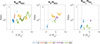 |
Fig. 8 Ratios of the estimated pick-up densities of SO+, S+, and |


3.6 Other species
Up to this point, we have concentrated on sulfur-bearing atoms and molecules coming from Io. The sampling rate of the magnetometer constrains the ion mass that can be detect to species heavier than O+ (i.e., mpu > 16 u). Russell & Kivelson (2001) have shown evidence of, for instance, chlorine (Cl, 35 and 37 u), also found around Europa by Volwerk et al. (2001). It is well known that near Io there is also sodium (Na; 23 u), potassium (K; 39 u; Trafton et al. 1974; Summers et al. 1983; Thomas 1996), and possibly chlorine (Cl; 35 u and 37 u) and hydrogensulfide (H2S; 34 u; Russell & Kivelson 2001). Na et al. (1998) proposed a list of heavy neutral species that may be present in Io’s atmosphere, which could be detected with ground-based observations between 320 and 440 nm. The list includes Na and Si. Moses et al. (2002) discussed the photo-chemistry in Io’s atmosphere for alkalis and chlorine, listing Na and K, which are also discussed by Redwing et al. (2022).
The spectral analysis of the magnetometer data does indeed reveal additional ion species. Based on the mentioned “other” species above, we searched for ICW power for 35Cl+, 37Cl+, H2S+/34S+, K+, and Si+. The results are shown in Fig. 10, except for Na+, which did not produce any wave signature and with the addition of a species of mass ∼31 u, which we identified as plausibly P+.
From the line spectra in Fig. 9, it is clear that the peaks for the lighter ion species are closer together in frequency. In order to obtain the spectral power in each peak, the limits of the frequency window have been changed to
![Mathematical equation: ${W_{{\rm{freq,others}}}} = [W(1),W(2)] = \left[ {0.97\left( {{f_{\rm{c}}} - {\rm{\Delta }}{f_{\rm{c}}}} \right),{f_{\rm{c}}} + {\rm{\Delta }}{f_{\rm{c}}}} \right].$](/articles/aa/full_html/2026/04/aa56518-25/aa56518-25-eq63.png) (14)
(14)
There is a large range of pick-up rates for the different species and the different flybys. The different colors that dominate the plots for the various flybys show also that not every species is detected during each flyby. We note that some ion species are close in mass (e.g., 35Cl+ and H2S+) are only 1 u apart. It could well be that some wave power may bleed over because of the frequency window that is used (Eq. (14)), but the spectral resolution does distinguish between these ions (see the discussion in Sect. 3.9). In Fig. 9, two line spectra are shown from the I27 and I31 flybys. The colored vertical lines show the cyclotron frequencies of the “other” species (see legend for the ion species). This plot shows that indeed 35Cl+ and H2S+/34S+ can be distinguished, but comparing the two panels shows that not every species shows activity. In I27, there is a peak just below the 35Cl+ frequency and in I31 a peak at the H2S+/34S+ frequency. Panels A and E of Fig. 10 show similarities in the curves; however, with 35Cl+ at lower Npu values and a steeper fall-off than for H2S+/34S+. The ratio of these two ions, NH2S/NCl (not shown) is not constant and slowly increases with increasing X from ∼2.5 to ∼4.5 for I27.
Two different isotopes of chlorine (35 and 37 u) are present. The locations of the emissions along the corotating flow differ quite strongly. This is partly is because of the orbits; I0 and I24 do not extend far down tail as mentioned earlier. Emissions attributed to the two isotopes in the I27 flyby drop-off faster for 37Cl+ than for I32 and this isotope appears further downstream. Also, there seems to be more 37Cl+ during the I24 flyby. I31 shows similar pick-up densities for both isotopes.
Potassium, (K, mass 39 u), is observed on all flybys except I24. I0 shows ICW power within 0 ≤ X ≤ 1, the strongest power is near Y ≈ 2.8 and a weaker patch of emissions occurs within −5.6 ≤ Y ≤ 4. For the other flybys the deduced pick-up density decreases slowly. On I31, pick-up signatures appear only quite far downstream of Io. Dihydrogensulfide (H2S, mass 34 u) or 34S is mainly present during the I27 flyby and a small patch is present during the I31 flyby. Potassium (Fig. 10 panel B) is concentrated around Io for I24, but for I27/31/32 emissions are only present downstream. The limited region of emission for I24 most likely represents the end of the high-resolution data. Silicon (mass 28 u) is basically present only during the I27 flyby. There is ICW power at a frequency corresponding to a mass of 31 u, which we identified as phosphorus.
Interestingly, it is only during the I27 flyby that we can see an extended curve of emissions for all ions from X ≈ 1.5 to X ≈ 7.5, where the curves end at the end of the high-resolution magnetometer data. The I32 flyby shows that up to X ≈ 8 there is a pick-up ion density for K+, however, other ion species show up only sporadically.
As the I0 flyby had a quite different geometry than those of the other flybys, the species detected along the Y-direction is shown in Fig. 11. The sulfur-bearing species are plotted in black lines, and appear on both the anti-Jovian and the sub-Jovian sides of Io. The “other” species are mainly observed between −6 ≤ Y ≤ −4, with a small patch for K+ and 37Cl+ near Y ≈ −3.
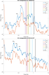 |
Fig. 9 Two line spectra for the I27 and I31 flybys. Shown are the perpendicular (blue) and parallel (red) power spectra. The colored vertical lines indicate the “other” species (see legend). |
 |
Fig. 10 Estimated pick-up densities for 35Cl+, 37Cl+, K+, P+, H2S+, or 34S+ and Si+ as a function of XIΦO (same format as Fig. 7). |
3.7 Comparison with earlier detections
As mentioned before, pick-up ions, mainly the sulfur-bearing ions (but also chlorine) have previously been identified through ICWs. However, the identification of potassium, silicon, and phosphorus via ICWs are a first. Below, we give an overview of papers dealing with ICWs near Io and what species were identified in these studies.
Kivelson et al. (1996) discussed the presence of ICWs on I0’s ingress (before entering the geometrical wake) and egress (after exiting the geometrical wake), where they show peak frequencies varying between the SO+ and
 frequencies. They did not find any signatures of O+ and S+.
Huddleston et al. (1997) performed spectral analysis on data from the I0 flyby and found that the strongest signal came from
 . Calculating the warm-plasma dispersion relation, they found that the heaviest pick-up ions are most likely to generate an unstable ring distribution and thereby allow for the growth of ICWs.
Warnecke et al. (1997) also studied the I0 flyby and found ICWs near the
 gyrofrequency and occasionally near the SO+ gyrofrequency.
Russell et al. (1998) studied a longer interval along the I0 flyby (1707–1801 UT) and determined, for 7 min intervals, the peak ICW frequency and from that derived the respective mass of the pick-up ions. This mass varied from 51 ≤ mpu ≤ 67 on ingress to 41 ≤ mpu ≤ 73 on egress (see their Table 1). They noticed the asymmetry in the wave signatures inbound and outbound from Io, arguing for a strong
 pick-up on the dayside.
Russell & Kivelson (2001) studied the flybys I0, I24, I25 (for which the spacecraft had a “safing event” and data recording did not start until after closest approach), and I27 for the presence of pick-up ions. For the I27 flyby, they found evidence of already known ions as well as others: H2S+, 35Cl+, and 37Cl+.
Blanco-Cano et al. (2001b) performed wave dispersion analysis on the magnetometer data of the I0, I24, I27, and I31 flybys. In the data, they found the presence of
 and SO+, as well as S+ and H2S+, where SO+ had the strongest amplitude for all flybys. From the dispersion analysis, they found that ring distributions can generate IC wave growth, propagating along the field, but oblique propagation wave growth is also significant. The dominant mode is determined by features of the thermal background plasma in which the ions are picked up.
Blanco-Cano et al. (2001a) discuss the I0 flyby and find that
 ICWs propagate along the field, whereas SO+ and S+ propagate at an angle to the background magnetic field and are elliptically polarized.
Russell et al. (2003b) first discussed the I32 flyby and compared the ICW activity for all Io flybys. They observed that the ICWs mainly appear downstream of the moon, on either side (i.e., both on the anti- and sub-Jovian side) of Io’s orbit. The variability in the observed wave power for the different flybys were not related to the variable distance of Galileo to the moon, nor by the solar phase angle. The variations were most-likely produced by “varying styles and amplitudes of volcanic activity.”
Russell et al. (2003a) observed low-frequency cyclotron waves below the
 -frequency during the I31 flyby, which traversed the wake region of Io. The authors related these low frequencies to ion pick-up in the low field region downstream of Io that travel along the field lines to the spacecraft, but these waves also have a strong compressional component. They also observed higher-frequency waves, but these were not attributed to specific pick-up ions.
Cao et al. (2025) presented a study of the cyclotron wave amplitude around Io, using the five Galileo flybys. They found similar wave power in their dynamic spectra as in this current paper. However, they only discussed
 and SO+. Their conclusion is that the wave amplitudes decrease with increasing distance from Io. This finding is based on taking all measured amplitudes of all flybys and determining the median value along the corotational flow.
Cao et al. (2025) also discuss the wave power in the dynamic spectra from the (distant) Juno flybys of Io. The closest approaches during the Juno flybys PJ57 and PJ58 are approximately ten times further from Io than the Galileo flybys. They find that the spectral peaks seem to lie above the expected cyclotron frequency, but no explanation is given for this. Interestingly, the authors mainly concentrate on
 ICWs and did not use the higher Nyquist frequency to look for O+ ICWs or for species with smaller mass-to-charge ratio.
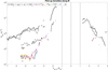 |
Fig. 11 Estimated pick-up densities for all ion species (see legend) as a function of YIΦO for the I0 flyby. |
3.8 Comparison with simulation results
Dols et al. (2012) and Dols (2025) simulated the five I0 flybys to study the asymmetry of Io’s outer atmosphere, using a code that “couples an MHD model of the flow and magnetic perturbations around the moon with a multispecies chemistry model that includes the physical chemistry of the main species.” Dols et al. (2024) improved the chemistry and also added processes arising from the field-aligned electron beams: Their results show a wake dominated by SO+ produced by the field-aligned electron beams (see their Fig. 15d).
For the I0 flyby they show the mixing ratio for  , SO+, S+, S2+, S3+, O+, and O2+ in their Fig. 22. They show that near Io
  is the dominant ion, but outside of |Y| > 2 other ions contribute to the plasma. However, SO+ is never more abundant than
  .
.
For the purposes of comparison with Dols et al. (2012) and Dols (2025), we show a plot with the pick-up densities along the I0 flyby along Y in Fig. 11. As mentioned above, we cannot obtain pick-up densities for O+. We can see that for |Y| < 2 the pick-up density of  dominates; further out, SO+ and K+ are dominant for a short interval during ingress, while
  , SO+, S+, and K+ dominate for short intervals during egress.
The variation in the pick-up density at either side of the moon is quite different. Looking at the  and SO+ curves, as a function of Y, we can make an estimate of the pick-up density gradient for |Y| > 2. For the anti-Jovian side, we find that ∆Npu/∆Y ≈ 5.2 × 10⁵ #/RIo; whereas on the sub-Jovian side ∆Npu/∆Y ≈ 9.7 × 10⁵ #/RIo. Thus, the pick-up density on the sub-Jovian side falls off twice as fast as on the anti-Jovian side. This agrees well with the reported 45% higher column density at the anti-Jovian side than at the sub-Jovian side (Walker et al. 2012), as discussed above.
3.9 Uncertainties in density determination
We used the Galileo magnetometer data to search for ICWs of various ion species through spectral analysis. From the determined PSD we calculate the total power in the waves around the specific cyclotron frequency. With the assumption that the pickup ions completely transfer their energy to the waves (Φ = 1), we obtained a lower limit for the pick-up density.
In Fig. 12, we show a zoom-in of the line spectrum of I27 in Fig. 9, and have included the windows, Wfreq,others, for the different ion species in dashed vertical lines. This figure shows the possible bleeding of power from one peak into another. This means that from this point of view, the lower limit of the pick-up ion densities we determined through Φ = 1 is also an upper limit with respect to the spectral power in the spectral peaks. We note that not at all marked ion cyclotron frequencies an actual ICW event is found, as there are more conditions to the identification of ICWs as described in Sect. 2.3. The limitations to the determination of the pick-up ion densities, set by the actual unknown efficiency factor Φ and by the tuning of the integration window around the specific ion cyclotron frequencies, should be kept in mind when using this spectral technique.
 |
Fig. 12 Zoom-in on the line spectrum of I27 in Fig. 9. The solid vertical lines show the cyclotron frequencies and the dashed vertical lines show the window over which the spectral power in the peak is calculated. |
4 Further limitations of the technique
This species-identification method, based on ICWs, is dependent on the mass-to-charge ratio of the picked-up ions which determines their cyclotron frequency, as expressed in Eq. (1). This means that ions with the same mass-to-charge ratio cannot be identified, a limitation that is often found for many separate plasma instruments (see, e.g., Haggerty et al. 2017; Roussos et al. 2022).
Ions with small differences in mass can be separated in the spectral analysis, but we cannot exclude the possibility that because of the chosen frequency window size when integrating the wave power from the PSD, there can be some leakage of spectral power from species with approximately the same mass-to-charge ratio. Visual inspection of the window size should always be performed.
Another limitation is the available data rate of the magnetometer and the associated Nyquist frequency. As shown in this paper, the three (or four for I0) vectors per second resolution prohibits the detection of O+ ICWs. In newer missions, the data rate is often higher and, thus, lighter ions (from oxygen downwards) can be identified; for example, in the Juno magnetometer data.
The presence of other ions with a temperature anisotropy can lead to wave growth suppression. As an example, in the Earth’s magnetosheath the “regular” conditions for the proton cyclotron instability can be fulfilled, as measured, for example, by the AMTPE/CCE (Anderson & Fuselier 1993; Anderson et al. 1994). However, through the presence of a tenuous He++ component, the threshold temperature anisotropy is changed (Gary et al. 1994; Fuselier et al. 1994). Therefore, in specific studies, it may be useful to apply a wave dispersion solver, as in the case of “Bo” (Xie 2019). This would allow us to check whether growth rates are suppressed in a multicomponent plasma and whether the pick-up densities might be underestimated.
5 Discussion
We used the previously applied method of determining pickup ions through magnetometer measurements of ion cyclotron waves (Huddleston et al. 1998; Volwerk et al. 2001; Schmid et al. 2022, 2025). For a review of this method around various planets and comets, we refer to Lammer et al. (2025). As in previous studies, we assumed that the background plasma has a distribution close to a Maxwellian and that pick-up ions create a “bump in tail” that is unstable to wave growth (see, e.g., Melrose 1986 and Treumann & Baumjohann 2018, both Sect. 4.1). This assumption is more likely to be correct for the dominant ion species, but we adopted it for all ions. The pickup ions, which create a ring-beam distribution in velocity space, will resonate with the appropriate waves in the background turbulent wave spectrum (see Eq. (2)) and ion cyclotron waves will start to grow.
The presence of a thermal background of ions with the same mass-to-charge ratio will hamper wave growth through cyclotron Landau damping (Gary 1992). This means that to obtain wave growth sufficient pick-up needs to take place. The main thermal ions in the Io plasma torus are O+, O++, S+, S++, and S+++, which are created out of the dissociative ionization of the SO2 and SO originating from Io’s atmosphere (Bagenal 1994; Delamere & Bagenal 2003). Blanco-Cano et al. (2001a) did not consider a thermal background of  and SO+ because they assume a fast dissociation of these ions. Delamere & Bagenal (2003) also did not have a background density of these ions in their torus model. Growth of waves originating from the pick-up of S+ and O+ will be impeded by the background plasma. Blanco-Cano et al. (2001b) performed dispersion calculations and found that; for example, the density of the ring-beam pick-up ions of S+ should be ≥ 10% of the thermal background density of S+ to get significant wave growth.
For all five Io flybys by the Galileo spacecraft for which magnetometer data were available, we performed spectral analysis to determine the presence of ICWs from the sulfur-bearing species:  ,
,  , SO+, and S+. These can be well separated in spectral analysis. With the assumption that free energy in the ring-beam distribution (Eq. (5)) is fully transferred to the ICWs (Φ = 1), we obtained a lower limit for the pick-up ion densities, because the efficiency could be as low as Φ = 0.3 (Cowee et al. 2007); however, this might be dependent on the pick-up ion species. Cowee et al. (2007) investigated the growth of H2O+ ICWs at comets and predicts Φ = 0.25 for
  at Io. As expected, the determined pick-up densities decrease with increasing distance from Io, mainly in the region outside of Io’s orbit and downstream of the moon. The inferred pick-up densities for the different species and the different flybys vary between ∼105 and ∼108 m−3.
As in the case of Europa (Volwerk et al. 2001), species that contain no sulfur are also ionized near Io and picked-up by the Jovian magnetic field. We found evidence of 35Cl+, 37Cl+, K+, H2S+/34S+, Si+, and, possibly, P+ (at least a mass ∼31 u ion). Interestingly, there seems to be no signature of Na+, even though there is a large sodium cloud around Io. The lack of signatures is probably caused by a thermal background of Na+ (Wilson et al. 2002; Bagenal & Dols 2020). Some additional species are not picked-up on all flybys, as shown in Fig. 10. The I27 flyby shows that there is pick-up of all “other” ions along a very extended path, which is in stark contrast to the other flybys (Fig. 10).
The results obtained in this paper are in general agreement with earlier studies of ion cyclotron waves (Warnecke et al. 1997; Huddleston et al. 1998; Russell et al. 1998, 1999; Huddleston et al. 1999; Russell & Kivelson 2001), altough these studies mainly concentrated on the sulfur-bearing ions. However, our results do not completely in agreement with previous studies, specifically at the locations where the ICWs of the sulfur-bearing ions are found. This happens because of the strict identification constraints we set onto the data analysis, as given in Sect. 2.3.
Because of the different System III longitudes of the different flybys, Io is embedded in different background plasmas inside the plasma torus. Also, the Jovian local times were quite different (Table 1) and our results show that this all together makes a great difference in the pick-up densities around Io. These vary by up to an order of magnitude, but apparently not for the dominant pick-up of SO+, which shows values that agree well between the different flybys.
If the discovered element, with mass 31, is indeed phosphorus, an essential element for life as we know it and for the habitability of planets in general (e.g., Cockell et al. 2011; Westheimer 1987), our discovery may have important implications for the neighboring icy moons Europa, Ganymede, and Callisto. On planetary bodies beyond Earth, P has so far only been observed in the environment of Saturn’s moon Enceladus, where it originates from phosphates in the moon’s sub-surface water ocean (Postberg et al. 2023). On Io, P would be ejected into the moon’s environment from the planet’s interior by volcanoes. Since all four Galilean moons formed by accretion from a protoplanetary disk around Jupiter, our detection would suggest, as in the case of Saturn’s moon Enceladus, that P may also be present as orthophosphates (e.g.,  , Hao et al. 2022) in the subsurface water oceans of Europa, Ganymede, and Callisto. Moreover, future studies on the presence of phosphorus in the Jovian system, such as in Io’s environment or the other moons, along with its presence on Saturn’s moon Enceladus, could help us understand how this bio-essential element is distributed and cycled throughout the Solar System.
Recently, Cao et al. (2025) presented a study of the cyclotron wave amplitude around Io, using both the five Galileo flybys and the two Juno flybys of Io. Using very loose criteria for the determination of ICWs (ellipticity smaller than 0, wave vector angle with the background magnetic field less than 70◦), they found similar wave power in their dynamic spectra as in this current paper. However, they only discussed  and SO+ in that work. Their conclusion is that the wave amplitudes decrease with increasing distance from Io. This is based on taking all measured amplitudes of all flybys and determining the median value along the corotational flow. As is clear from the variations in the pick-up densities determined in this current paper, this cannot be done for the reasons mentioned above. The wave power in the dynamic spectra of the Juno flybys seems to lie above the expected cyclotron frequency, but no explanation is given for this in the Cao et al. (2025) study.
Although this paper deals only with the Galileo flybys of Io, a preliminary investigation of the PJ57 Io flyby by Juno has also been performed. It was shown that the measured ICW frequencies were approximately 15% higher than the local ICW frequency determined from the background magnetic field. This can be explained by non-local pick-up and generation of the waves (and thus no anomalous Doppler effect) and then a Doppler shift to higher frequencies as the waves are transported by the plasma flow. Further investigations of the Juno data are underway by A. Große-Schware (personal communication).
6 Conclusions
Ion cyclotron waves can be used to estimate the ion pick-up around Io (or any other moon or planet) based on the assumption of a background plasma distribution that falls smoothly as a function of energy. This is a good tool to complement observations by plasma instruments, albeit with its own limitations, as discussed in Sect. 4.
We have shown that there is a large variety of pick-up ions around Io over a large region downstream of the moon, which means that there is an extensive neutral atmosphere and exosphere. We have identified pick-up signatures, ICWs, of the sulfur-bearing ions  ,
,  , SO+, S+, and H2S+ or 34S+, as well as of the non-sulfur-bearing ions 35Cl+, 37Cl+, K+, Si+, and P+. Although there is an extended sodium cloud around Io, no ICWs were detected at the local Na+ gyrofrequency. This was most likely caused by the large thermal population of Na+ suppressing the wave growth. The first identification of phosphorus in Io’s emissions strengthens the possibilities for habitats in the Jovian system, thereby opening a new window for the current JUICE and Europa Clipper missions to Jupiter.
Acknowledgements
Vincent Dols is supported by the NASA NFDAP 2020-0014 Grant 80NSSC21K0825, the NASA Solar System 999 Workings 2020-0139 Grant 80NSSC22K0109 and also supported at the University of Colorado as 1000 a part of NASA’s Juno mission supported by NASA through contract 699050 with the Southwest 1001 Research Institute. The work by Cyril Simon Wedlund was funded by the Austrian Science Fund (FWF) under grant number 10.55776/P35954. Anatol Große-Schware acknowledges support from the Swedish National Space Agency through grant 2023-00222. The Galileo data are available from NASA’s Planetary Data System (PDS): the magnetometer data at https://doi.org/10.17189/1gfw-1y75.
References
- Anderson, B. J., & Fuselier, S. A. 1993, J. Geophys. Res., 98, 1461 [Google Scholar]
- Anderson, B. J., Fuselier, S. A., Gary, S. P., & Denton, R. E. 1994, J. Geophys. Res., 99, 5877 [NASA ADS] [CrossRef] [Google Scholar]
- Arthur, C., McPherron, R. L., & Means, J. D. 1976, Radio Sci., 11, 833 [Google Scholar]
- Bagenal, F. 1994, J. Geophys. Res., 99, 11043 [NASA ADS] [CrossRef] [Google Scholar]
- Bagenal, F., & Dols, V. 2020, J. Geophys. Res., 125, e2019JA027485 [Google Scholar]
- Blanco-Cano, X., Russell, C. T., Huddleston, D. E., & Strangeway, R. J. 2001a, Planet. Space Sci., 49, 1125 [Google Scholar]
- Blanco-Cano, X., Russell, C. T., & Strangeway, R. J. 2001b, J. Geophys. Res., 106, 26261 [Google Scholar]
- Brain, D. A., Bagenal, F., Acuña, M. H., et al. 2002, J. Geophys. Res., 107, 1076 [Google Scholar]
- Brinca, A. L. 1991, in Cometary Plasma Processes, Geophys. Monogr. Ser., 61, ed. A. D. Johnstone (Washington, DC, USA: AGU), 211 [Google Scholar]
- Buratti, B. J., Mosher, J. A., & Terrile, R. J. 1995, Icarus, 118, 418 [Google Scholar]
- Cao, X., Wang, S., Ni, B., et al. 2025, Geophys. Res. Lett., 52, e2025GL115547 [Google Scholar]
- Chou, M., & Cheng, C. Z. 2017, Earth Planet Space, 69, 122 [Google Scholar]
- Cockell, C. S., Bush, T., Direito, S., et al. 2011, Astrobiology, 165, 89 [Google Scholar]
- Connerney, J. E. P., Acuna, H. M., & Ness, N. F. 1981, J. Geophys. Res., 87, 8370 [Google Scholar]
- Connerney, J. E. P., Benn, M., Bjarno, J. B., et al. 2017, Space Sci. Rev., 213, 39 [Google Scholar]
- Cowee, M. M., Winske, D., Russell, C. T., & Strangeway, R. J. 2007, Geophys. Res. Lett., 34, L02113 [Google Scholar]
- Crary, F. J., & Bagenal, F. 2000, J. Geophys. Res., 105, 25379 [Google Scholar]
- de Kleer, K., de Pater, I., & Ádámkovics, M. 2019, Icarus, 317, 104 [Google Scholar]
- de Pater, I., Luszcz-Cook, S., Roja, P., et al. 2020, Planet. Sci. J., 1, 60 [NASA ADS] [CrossRef] [Google Scholar]
- de Pater, I., Lellouch, E., Strobel, D. F., et al. 2023, J. Geophys. Res., 128, e2023JE007872 [Google Scholar]
- Delamere, P. A., & Bagenal, F. 2003, J. Geophys. Res., 108, 1276 [Google Scholar]
- Delva, M., Mazelle, C., & Bertucci, C. 2011, Space Sci. Rev., 162, 5 [Google Scholar]
- Delva, M., Zhang, T. L., Volwerk, M., Vörös, Z., & Pope, S. A. 2008, Geophys. Res. Lett., 113, E00B06 [CrossRef] [Google Scholar]
- Delva, M., Bertucci, C., Volwerk, M., et al. 2015, J. Geophys. Res., 120, 344 [NASA ADS] [CrossRef] [Google Scholar]
- Dols, V. 2025, J. Geophys. Res., 130, e2025JA033798 [Google Scholar]
- Dols, V., & Johnson, R. E. 2023, Icarus, 392, 115365 [Google Scholar]
- Dols, V., Delamere, P. A., Bagenal, F., Kurth, W. S., & Paterson, W. R. 2012, J. Geophys. Res., 117, E10010 [Google Scholar]
- Dols, V., Paterson, W. R., & Bagenal, F. 2024, J. Geophys. Res., 129, e2023JA031763 [Google Scholar]
- Fowler, R. A., Kotick, B. J., & Elliott, R. D. 1967, J. Geophys. Res., 72, 2871 [NASA ADS] [CrossRef] [Google Scholar]
- Fuselier, S. A., Anderson, B. J., Gary, S. P., & Denton, R. E. 1994, J. Geophys. Res., 99, 14931 [Google Scholar]
- Gary, S. P. 1991, Space Sci. Rev., 56, 373 [NASA ADS] [CrossRef] [Google Scholar]
- Gary, S. P. 1992, J. Geophys. Res., 97, 8519 [NASA ADS] [CrossRef] [Google Scholar]
- Gary, S. P., Fuselier, S. A., & Anderson, B. J. 1993, J. Geophys. Res., 98, 1481 [NASA ADS] [CrossRef] [Google Scholar]
- Gary, S. P., Convery, P. D., Denton, R. E., Fuselier, S. A., & Anderson, B. J. 1994, J. Geophys. Res., 99, 5915 [Google Scholar]
- Gary, S. P., Liu, K., & Chen, L. 2012, J. Geophys. Res., 117, A08201 [Google Scholar]
- Haggerty, D. K., Mauk, B. H., Paranicas, C. P., et al. 2017, Geophys. Res. Lett., 44, 6476 [Google Scholar]
- Hao, J., Glein, C. R., Huang, F., et al. 2022, PNAS, 119, e2201388119 [Google Scholar]
- Hasegawa, A. 1969, Phys. Fluids, 12, 2642 [CrossRef] [Google Scholar]
- Huddleston, D. E., & Johnstone, A. D. 1992, J. Geophys. Res., 97, 12217 [NASA ADS] [CrossRef] [Google Scholar]
- Huddleston, D. E., Strangeway, R. J., Warnecke, J., et al. 1997, Geophys. Res. Lett., 24, 2143 [Google Scholar]
- Huddleston, D. E., Strangeway, R. J., Warnecke, J., Russell, C. T., & Kivelson, M. G. 1998, J. Geophys. Res., 103, 19887 [Google Scholar]
- Huddleston, D. E., Strangway, R. J., Blanco-Cano, X., et al. 1999, J. Geophys. Res., 104, 17479 [Google Scholar]
- Huddleston, D. E., Strangeway, R. J., Blanco-Cano, X., et al. 2000, Adv. Space Sci., 26, 1513 [Google Scholar]
- Kivelson, M. G., Khurana, K. K., Means, J. D., Russell, C. T., & Snare, R. C. 1992, Space Sci. Rev., 60, 357 [Google Scholar]
- Kivelson, M. G., Kurana, K. K., Walker, R. J., et al. 1996, Science, 273, 396 [Google Scholar]
- Klaasen, K., Belton, M., Breneman, H., et al. 1997, Opt. Eng., 38, 3001 [Google Scholar]
- Kupo, I., Mekler, Y., & Eviatar, A. 1976, Astrophys. J. Lett., 205, L51 [Google Scholar]
- Lammer, H., Schmid, D., Volwerk, M., et al. 2025, Front. Astron. Space Sci., 11, 14999346 [Google Scholar]
- Leisner, J. S., Russell, C. T., Dougherty, M. K., et al. 2006, Geophys. Res. Lett., 33, L11101 [Google Scholar]
- Long, M., Cao, X., Gu, X., et al. 2022, Astrophys. J., 932, 56 [Google Scholar]
- Lucek, E. A., Dunlop, M. W., Balogh, A., et al. 1999, Ann. Geophys., 17, 1560 [NASA ADS] [CrossRef] [Google Scholar]
- Mazelle, C., & Neubauer, F. M. 1993, Geophys. Res. Lett., 20, 153 [NASA ADS] [CrossRef] [Google Scholar]
- Means, J. D. 1972, J. Geophys. Res., 77, 5551 [NASA ADS] [CrossRef] [Google Scholar]
- Melrose, D. B. 1986, Instabilities in Space and Laboratory Plasmas (Cambridge, UK: Cambridge University Press) [Google Scholar]
- Moses, J. I., Zolotov, M. Y., & Fegley, B. Jr., 2002, Icarus, 156, 107 [Google Scholar]
- Na, C. Y., Trafton, L. M., Barker, E. S., & Stern, S. A. 1998, Icarus, 131, 449 [Google Scholar]
- Postberg, F., Sekine, Y., Klenner, F., et al. 2023, Nature, 618, 489 [NASA ADS] [CrossRef] [Google Scholar]
- Radulescu, C. R., Coates, A. J., Simon, S., Verscharen, D., & Jones, G. H. 2025, J. Geophys. Res., 130, e2024JA033390 [Google Scholar]
- Redwing, E., de Pater, I., Luszcz-Cook, S., et al. 2022, Planet. Sci. J., 3, 238 [Google Scholar]
- Rönnmark, K. 1982, Rep. Kiruna Geophys. Inst., 179 [Google Scholar]
- Roussos, E., Cohen, C., Kollmann, P., et al. 2022, Sci. Adv., 8, eabm4234 [Google Scholar]
- Russell, C. T., & Kivelson, M. G. 2001, J. Geophys. Res., 106, 33267 [Google Scholar]
- Russell, C. T., Luhmann, J. G., Schwingenschuh, K., & Ye, Y. 1990, Geophys. Res. Lett., 17, 897 [NASA ADS] [CrossRef] [Google Scholar]
- Russell, C. T., Kivelson, M. G., Khurana, K. K., & Huddleston, D. E. 1998, Planet. Space Sci., 47, 143 [Google Scholar]
- Russell, C. T., Huddleston, D. E., Strangeway, R. J., et al. 1999, J. Geophys. Res., 104, 17471 [Google Scholar]
- Russell, C. T., Blanco-Cano, X., & Kivelson, M. G. 2003a, Planet. Space Sci, 51, 233 [Google Scholar]
- Russell, C. T., Blanco-Cano, X., Wang, Y. L., & Kivelson, M. G. 2003b, Planet. Space Sci., 51, 937 [Google Scholar]
- Samson, J. C., & Olson, J. V. 1980, Geophys. J. Int., 88, 115 [Google Scholar]
- Schmid, D., Narita, Y., Plaschke, F., et al. 2021, Geophys. Res. Lett., 48, e2021GL092606 [CrossRef] [Google Scholar]
- Schmid, D., Lammer, H., Plaschke, F., et al. 2022, J. Geophys. Res., 127, e2022JE007462 [Google Scholar]
- Schmid, D., Lammer, H., Berezhnoy, A. A., et al. 2025, Nat. Commun., 16, 6205 [Google Scholar]
- Schneider, N. M., & Trauger, J. T. 1995, Astrophys. J., 450, 450 [Google Scholar]
- Simonelli, D. P., Veverka, J., Senske, D. A., et al. 1998, Icarus, 135, 166 [Google Scholar]
- Smith, E. J., & Tsurutani, B. T. 1983, J. Geophys. Res., 88, 7831 [Google Scholar]
- Sonnerup, B. U. Ö., & Scheible, M. 1998, in Analysis Methods for Multi-Spacecraft Data, eds. G. Paschmann, & P. Daly (Noordwijk: ESA), 185 [Google Scholar]
- Southwood, D. J., & Kivelson, M. G. 1993, J. Geophys. Res., 98, 9181 [NASA ADS] [CrossRef] [Google Scholar]
- Spencer, J. R., Lellouch, E., Richter, M. J., et al. 2005, Icarus, 176, 283 [Google Scholar]
- Summers, M. E., Yung, Y. L., & Haff, P. K. 1983, Nature, 304, 710 [Google Scholar]
- Thomas, N. 1996, Astron. Astrophys., 313, 306 [Google Scholar]
- Trafton, L., Parkinson, T., & Macy, W., Jr. 1974, Astrophys. J., 190, L85 [Google Scholar]
- Treumann, R. A., & Baumjohann, W. 2018, Ann. Geophys., 36, 1015 [NASA ADS] [CrossRef] [Google Scholar]
- Tsang, C. C. C., Spencer, J. R., Lellouch, E., et al. 2013, Icarus, 226, 1177 [Google Scholar]
- Tsang, C. C. C., Spencer, J. R., Lellouche, E., Lopez-Valverde, M. A., & Richter, M. J. 2016, J. Geophys. Res., 121, 1400 [Google Scholar]
- Vasyliunas, V. M. 1975, Geophys. Res. Lett., 2, 87 [Google Scholar]
- Volwerk, M., & Khurana, K. K. 2010, in Pickup ions throughout the heliosphere and beyond, AIP conference proceedings, 1302, eds. J. A. le Roux, V. Florinski, & G. P. Zank (Melville, NY, USA: IAP), 263 [Google Scholar]
- Volwerk, M., Kivelson, M. G., & Khurana, K. K. 2001, J. Geophys. Res., 106, 26033 [Google Scholar]
- Walker, A. C., Moore, C. H., Goldstein, D. V., Varghese, P. L., & Trafton, L. M. 2012, Icarus, 220, 225 [Google Scholar]
- Warnecke, J., Kivelson, M. G., Khurana, K. K., Huddleston, D. E., & Russell, C. T. 1997, Geophys. Res. Lett., 24, 2139 [Google Scholar]
- Weichbold, F., Lammer, H., Schmid, D., et al. 2025, J. Geophys. Res., 130, e2024JE008679 [Google Scholar]
- Westheimer, F. H. 1987, Science, 235, 1173 [Google Scholar]
- Wilson, J. K., Mendillo, M., Baumgardner, J., et al. 2002, Icarus, 157, 476 [Google Scholar]
- Xie, H.-S. 2019, Comp. Phys. Comm., 244, 343 [Google Scholar]
IΦO is defined relative to the location of Io at Galileo’s closest approach, with the X-axis in the direction of corotation, the Z-axis along Jupiter’s rotational axis, and the Y-axis completes the right-handed system pointing roughly towards Jupiter. https://pds-ppi.igpp.ucla.edu/
All Tables
All Figures
|
Fig. 1 Five Io flybys used in this study for which magnetometer data are available. The orbits are shown as dotted lines projected onto the IΦO YX-plane (top) and YZ-plane (bottom). The solid intervals show the region over which high-resolution magnetometer data are available. The two dashed black lines at YIΦO = ±1 show the geometrical wake downstream of Io. |
| In the text | |
|
Fig. 2 Overview of the I0 flyby. The spectrograms show the perpendicular power density, polarization, ellipticity, and polar angle. The white lines show the cyclotron frequency of S+ (dotted), SO+ (dashed) |
| In the text | |
|
Fig. 3 Details about the orange, red, and purple boxes in Fig. 2. The orange box shows an interval with |
| In the text | |
|
Fig. 4 Five Io flybys in local time around Jupiter. The orbits of Galileo are shown as solid lines that start at the circle and end at the asterisk. |
| In the text | |
|
Fig. 5 Spectral analysis of the I24, I27, I31, and I32 Io flybys. The local cyclotron frequencies for |
| In the text | |
|
Fig. 6 Estimated pick-up ion densities in the IΦO YX and YZ planes. |
| In the text | |
|
Fig. 7 Estimated pick-up densities for |
| In the text | |
|
Fig. 8 Ratios of the estimated pick-up densities of SO+, S+, and |
| In the text | |
|
Fig. 9 Two line spectra for the I27 and I31 flybys. Shown are the perpendicular (blue) and parallel (red) power spectra. The colored vertical lines indicate the “other” species (see legend). |
| In the text | |
|
Fig. 10 Estimated pick-up densities for 35Cl+, 37Cl+, K+, P+, H2S+, or 34S+ and Si+ as a function of XIΦO (same format as Fig. 7). |
| In the text | |
|
Fig. 11 Estimated pick-up densities for all ion species (see legend) as a function of YIΦO for the I0 flyby. |
| In the text | |
|
Fig. 12 Zoom-in on the line spectrum of I27 in Fig. 9. The solid vertical lines show the cyclotron frequencies and the dashed vertical lines show the window over which the spectral power in the peak is calculated. |
| In the text | |
Current usage metrics show cumulative count of Article Views (full-text article views including HTML views, PDF and ePub downloads, according to the available data) and Abstracts Views on Vision4Press platform.
Data correspond to usage on the plateform after 2015. The current usage metrics is available 48-96 hours after online publication and is updated daily on week days.
Initial download of the metrics may take a while.