Shedding the envelope: JWST reveals a kiloparsec-scale [O III]-weak Balmer shell around a z = 7.64 quasar

Julien Wolf; Eduardo Bañados; Xiaohui Fan; Antoine Dumont; James E. Davies; David S. N. Rupke; Jinyi Yang; Weizhe Liu; Silvia Belladitta; Aaron Barth; Sarah Bosman; Tiago Costa; Frederick B. Davies; Roberto Decarli; Dominika Ďurovčíková; Anna-Christina Eilers; Hyunsung D. Jun; Yichen Liu; Federica Loiacono; Alessandro Lupi; Chiara Mazzucchelli; Maria Pudoka; Sofía Rojas-Ruiz; Jan-Torge Schindler; Wei Leong Tee; Benny Trakhtenbrot; Fabian Walter; Huanian Zhang

doi:10.1051/0004-6361/202557934

Open Access

Issue		A&A Volume 707, March 2026


Article Number		A299
Number of page(s)		19
Section		Extragalactic astronomy
DOI		https://doi.org/10.1051/0004-6361/202557934
Published online		16 March 2026

A&A, 707, A299 (2026)

Shedding the envelope: JWST reveals a kiloparsec-scale [O III]-weak Balmer shell around a z = 7.64 quasar

Julien Wolf¹^★, Eduardo Bañados¹, Xiaohui Fan², Antoine Dumont¹, James E. Davies¹, David S. N. Rupke³^,4, Jinyi Yang⁵, Weizhe Liu², Silvia Belladitta¹, Aaron Barth⁶, Sarah Bosman¹^,7, Tiago Costa⁸, Frederick B. Davies¹, Roberto Decarli⁹, Dominika Ďurovčíková¹⁰, Anna-Christina Eilers¹⁰, Hyunsung D. Jun¹¹^,12, Yichen Liu², Federica Loiacono⁹, Alessandro Lupi¹³^,14^,8, Chiara Mazzucchelli¹⁵, Maria Pudoka², Sofía Rojas-Ruiz¹⁶, Jan-Torge Schindler¹⁷, Wei Leong Tee², Benny Trakhtenbrot¹⁸, Fabian Walter¹ and Huanian Zhang¹⁹

¹ Max-Planck-Institut für Astronomie, Königstuhl 17, D-69117 Heidelberg, Germany
² Steward Observatory, University of Arizona, 933 N. Cherry Ave, Tucson, AZ 85719, USA
³ Department of Physics, Rhodes College, 2000 North Parkway, Memphis, TN 38112, USA
⁴ Zentrum für Astronomie der Universität Heidelberg, Astronomisches Rechen-Institut, Mönchhofstr 12-14, D-69120 Heidelberg, Germany
⁵ Department of Astronomy, University of Michigan, 1085 S. University Ave., Ann Arbor, MI 48109, USA
⁶ Department of Physics and Astronomy, University of California, Irvine, 4129 Frederick Reines Hall, Irvine, CA 92697-4575, USA
⁷ Institute for Theoretical Physics, Heidelberg University, Philosophenweg 12, D-69120 Heidelberg, Germany
⁸ School of Mathematics, Statistics and Physics, Newcastle University, Newcastle upon Tyne NE1 7RU, UK
⁹ INAF – Osservatorio di Astrofisica e Scienza dello Spazio di Bologna, Via Gobetti 93/3, I-40129 Bologna, Italy
¹⁰ MIT Kavli Institute for Astrophysics and Space Research, 77 Massachusetts Avenue, Cambridge, MA 02139, USA
¹¹ Department of Physics, Northwestern College, 101 7th St SW, Orange City, IA 51041, USA
¹² School of Physics, Korea Institute for Advanced Study, 85 Hoegiro, Dongdaemun-gu, Seoul 02455, Republic of Korea
¹³ Como Lake Center for Astrophysics, DiSAT, Università degli Studi dell’Insubria, Via Valleggio 11, I-22100 Como, Italy
¹⁴ INFN, Sezione Milano-Bicocca, P.za della Scienza 3, I-20126 Milano, Italy
¹⁵ Instituto de Estudios Astrofísicos, Facultad de Ingeniería y Ciencias, Universidad Diego Portales, Avenida Ejercito Libertador 441, Santiago, Chile
¹⁶ Department of Physics and Astronomy, University of California, Los Angeles, 430 Portola Plaza, Los Angeles, CA 90095, USA
¹⁷ Hamburg Observatory, Gojenbergsweg 112, D-21029 Hamburg, Germany
¹⁸ School of Physics and Astronomy, Tel Aviv University, Tel Aviv 69978, Israel
¹⁹ Department of Astronomy, School of Physics, Huazhong University of Science and Technology, Luoyu Road, Wuhan, 430074 Hubei, China

^★ Corresponding author: This email address is being protected from spambots. You need JavaScript enabled to view it.

Received: 1 November 2025
Accepted: 9 January 2026

Abstract

Luminous quasars at the redshift frontier z > 7 serve as stringent probes of super-massive black hole (SMBH) formation and they are thought to undergo much of their growth obscured by dense gas and dust in their host galaxies. Fully characterizing the symbiotic evolution of SMBHs and hosts requires rest-frame optical observations that span spatial scales from the broad-line region (BLR) to the interstellar and circumgalactic medium (ISM and CGM). The James Webb Space Telescope (JWST) now provides the necessary spatially resolved spectroscopy to do so. However, the physical conditions that regulate the interplay between SMBHs and their hosts at the highest redshifts, especially the nature of early feedback phases, remain unclear. We present JWST/NIRSpec integral field unit (IFU) observations of J0313−1806 at z = 7.64, the most distant luminous quasar known. From the rest-frame optical spectrum of the unresolved quasar, we derived a black hole mass of M_BH = (1.63 ± 0.10)×10⁹ M_⊙ based on Hβλ4861 (Hβ) and an Eddington rate of λ = L/L_Edd = 0.80 ± 0.05, consistent with previous Mg IIλ2800-based estimates. J0313–1806 exhibits no detectable [O III] λλ4959, 5007 emission on nuclear scales (3σ upper limit equivalent width of [O III] λ5007 < 1.42 Å). Most remarkably, we did detect an ionized gas shell extending out to ∼1.8 kpc traced by Hβ emission that also lacks any significant [O III] λλ4959, 5007, with a 3σ upper limit on the [O III] λ5007 to Hβ flux ratio of log₁₀(F([O III])/F(Hβ)) = −1.15. Through photoionization modeling, we demonstrate that the extended emission is consistent with a thin, clumpy outflowing shell where [O III] is collisionally de-excited by dense gas. We interpret this structure as a fossil remnant of a recent blowout phase, providing evidence for episodic feedback cycles in one of the earliest quasars. These findings suggest that dense ISM phases may play a crucial role in shaping the spectral properties of quasars across cosmic time.

Key words: galaxies: high-redshift / quasars: supermassive black holes / quasars: individual: J0313-1806

© The Authors 2026

Open Access article, published by EDP Sciences, under the terms of the Creative Commons Attribution License (https://creativecommons.org/licenses/by/4.0), which permits unrestricted use, distribution, and reproduction in any medium, provided the original work is properly cited.

This article is published in open access under the Subscribe to Open model.

Open access funding provided by Max Planck Society.

1. Introduction

In the luminous quasar phase, the powerful panchromatic radiation of an active galactic nucleus (AGN) unambiguously traces the accretion of a supermassive black hole (SMBH) at the centers of galaxies. Through dedicated optical and near-infrared (NIR) surveys, quasars have been discovered at ever increasing redshifts, well within the first gigayear of the Universe (z > 5.6, e.g., Fan et al. 2001; Reed et al. 2015; Wu et al. 2015; Bañados et al. 2016, 2023; Jiang et al. 2016; Matsuoka et al. 2016, 2018a,b, 2019, 2022, 2025; Wang et al. 2017; Gloudemans et al. 2022; Wolf et al. 2024; Ighina et al. 2024; Belladitta et al. 2025). The SMBHs powering these distant quasars populate the extreme end of the black hole mass scale (10⁸ − 10¹⁰ M_⊙, e.g., Onoue et al. 2019; Yang et al. 2021; Farina et al. 2022; Mazzucchelli et al. 2023), thereby providing stringent constraints on the formation and evolution of the very first massive black holes (Inayoshi et al. 2020; Fan et al. 2023). Only a handful of quasars beyond z > 7 have been identified to date (Mortlock et al. 2011; Bañados et al. 2018; Yang et al. 2020; Wang et al. 2021). The scarcity of confirmed sources at the quasar redshift frontier is generally attributed to two main factors: (1) the intrinsic steep decline in the space density of luminous quasars with increasing redshift, as captured by the quasar luminosity function at z > 6 (e.g., Schindler et al. 2023; Matsuoka et al. 2023); and (2) the fact that quasars at z ∼ 7.1 − 7.5 exhibit optical/NIR colours that are nearly indistinguishable from those of Galactic L- and T-dwarfs (e.g., Hewett et al. 2006; Lodieu et al. 2007; Mortlock et al. 2009; Fan et al. 2023; Bañados et al. 2025a).

However, the recent discovery of reionization-era blazars (Belladitta et al. 2020; Ighina et al. 2024; Wolf et al. 2024; Bañados et al. 2025b; Marcotulli et al. 2025) suggests a third possibility for the rarity of z > 7 quasars: many of these objects may be systematically missed in rest-frame UV searches because they are undergoing obscured growth, enshrouded in dense gas and/or dust (e.g., Maiolino & Rieke 1995; Assef et al. 2015; Vito et al. 2019b; Ni et al. 2020; Lambrides et al. 2020; Gilli et al. 2022). The fraction of obscured quasars has been shown to increase with redshift (e.g., Buchner et al. 2015; Liu et al. 2017; Glikman et al. 2018; Lanzuisi et al. 2017; Vito et al. 2018; Iwasawa et al. 2020; Gilli et al. 2022; Peca et al. 2023). Indeed, from the Lyαλ1216 absorption profiles of quasars at z > 7, Davies et al. (2019) inferred extremely low radiative efficiencies (≤0.1%), which may indicate that these quasars remain obscured over nearly the entirety of their growth phases. They constrain the obscured fraction at z > 7 to > 82% at 95% credibility.

This opens an exciting perspective, pointing to the existence of a vast, yet largely unexplored, quasar population at cosmic dawn. Conversely, the few archetypal dust-unobscured, broad-line quasars discovered at z > 7 must have already cleared the line of sight to their nuclei and broad-line regions (BLR), perhaps through powerful feedback associated with the so-called “blowout phase” (e.g., Hopkins et al. 2006; Zakamska et al. 2016; Ishibashi et al. 2018; Lansbury et al. 2020; Vayner et al. 2025). Detecting observational signatures of such a recent blowout in the immediate environments of the highest-redshift quasars (e.g., fossil distributions of expelled dense gas or dust) would offer a robust anchor for embedding these extremely rare sources within a broader evolutionary sequence.

The James Webb Space Telescope (JWST, Gardner et al. 2006)/Near-Infrared Camera (NIRCam, Rieke et al. 2023) has ushered in a new era by enabling, for the first time, detection of rest-frame ultraviolet (UV) and optical emission from the host galaxies of quasars at z > 6 (Ding et al. 2022, 2023; Stone et al. 2023; Yue et al. 2024). To overcome the stark contrast between the unresolved, dominant quasar light and the compact, faint stellar continuum emission at these wavelengths and redshifts, a detailed model of the instrument’s point spread function (PSF) is essential (e.g., Mechtley et al. 2012). With advanced imaging PSF subtraction techniques, it is now possible to directly measure the host galaxy’s stellar mass from the extended continuum emission detected with JWST, and to compare it with the central SMBH mass to assess whether their growth was offset with respect to local scaling relations (e.g. Magorrian et al. 1998; Ferrarese & Merritt 2000; Gebhardt et al. 2000; Häring & Rix 2004; Kormendy & Ho 2013; Reines & Volonteri 2015; Habouzit et al. 2021). The JWST Near-Infrared Spectrograph Integral Field Unit (NIRSpec IFU, Böker et al. 2022) enables integral field spectroscopy over tens of kiloparsecs (kpc) around high-redshift quasars and AGN, providing simultaneous access to the host galaxy’s stellar continuum, the quasar spectrum (e.g., Loiacono et al. 2024), and gas kinematics in the quasar vicinity, revealing quasar feedback (e.g., Liu et al. 2024) and large-scale interactions with companion galaxies (e.g., Marshall et al. 2023, 2025; Decarli et al. 2024; Übler et al. 2024). Similarly to NIRCam, detailed PSF modeling techniques are required to disentangle the quasar from underlying gas emission (e.g., Wylezalek et al. 2022; Veilleux et al. 2023; Perna et al. 2023; Vayner et al. 2024; Marshall et al. 2023, 2025).

At z_[C II] = 7.6423, the quasar J031343.84−180636.4 (hereafter, J0313−1806) is currently the most distant system known in which the properties of a matured > 10⁸ M_⊙ SMBH, its host and direct environment can be studied in detail (Wang et al. 2021). The virial single-epoch estimate of the SMBH mass, M_BH, based on the broad Mg IIλ2800 emission line is (1.6 ± 0.4)×10⁹ M_⊙, and Atacama Large Millimeter Array (ALMA) observations indicate a high value for the cold dust mass, namely, ∼7 × 10⁷ M_⊙. From its [C II] λ157.6 μm emission, Wang et al. (2021) further derived a high star-formation rate SFR_[C II] = 40−240M_⊙ yr⁻¹. In its rest-frame UV spectrum, the object shows signatures of strong outflows through broad absorption lines in C IVλ1549, S IVλλ1394,1403, and (tentatively) in Mg IIλ2800 (up to 0.19c), as well as a significant blueshift of its C IVλ1549 broad emission line (∼3100 km s⁻¹). The immediate environment of this quasar is therefore expected to show complex kinematics.

We present a study aimed at resolving the kinematic structure of the extended, rest-frame optical ionized gas emission within ∼15 kpc of J0313−1806 in both spectral and spatial dimensions with the JWST/NIRSpec Integral Field Unit (IFU, Cycle 1 GO 1764). In Section 2, we describe the JWST/NIRSpec IFU observations of J0313–1806 and the associated data reduction. Section 3 focuses on the nuclear quasar spectrum, from which we derived the central SMBH properties. In Section 4, we detail our PSF subtraction procedure and recover the extended gas emission in the quasar’s immediate environment. Finally, in Section 5, we synthesize the results from the nuclear spectrum and the extended emission to set them in a broader physical context. We present our conclusions in Section 6.

Throughout this paper, we assume a concordance lambda cold dark matter (ΛCDM) cosmology with parameters: H₀ = 70 km s⁻¹, Ω_M = 0.3, and Ω_Λ = 0.7. With this cosmology, one arcsecond corresponds to 4.96 kpc in proper (physical) transverse distance at z = 7.64. All equivalent widths (EWs) are rest-frame measurements. All images are shown in the north-up, east-left convention.

2. Observations and data reduction

2.1. JWST/NIRSpec IFU pointings

We observed J0313−1806 and an associated PSF calibration star, TYC 5875-488-1, with JWST/NIRSpec IFU on Jan 21, 2023, as part of our JWST Cycle 1 proposal ID 1764. The total exposure times were 9.82 and 0.17 hours, respectively. The grating and filter combination G395M/F290LP covers wavelength range 2.87–5.10 μm with a nominal resolving power of R ∼ 1000. The velocity resolution of our cube is thus roughly 300 km s⁻¹. The field of view of JWST/NIRSpec IFU is 3″ × 3″ (corresponding to ∼15 kpc × 15 kpc at the redshift of the quasar), with a native pixel scale of 0.1″. The NIRSpec IFU PSF is undersampled by design. A small cyclic eight-point dithering pattern was chosen to improve spatial sampling. This observing strategy alleviates aliasing effects arising from the undersampled PSF (so-called wiggles, e.g., Perna et al. 2023). Each dither consists of three integrations of 20 groups each. The readout pattern was set to NRSIRS2. In addition to the cyclic dithers, an additional leakcal exposure was taken to monitor and correct for light leaks from the neighbouring micro-shutter-array (MSA) on JWST.

2.2. Data reduction

We reduced the data cubes with the standard three-stage JWST Science Calibration Pipeline¹ version 1.15.0 (CRDS context: jwst_1322.pmap). The first stage, calwebb_detector1, performs group-level corrections on uncalibrated data such as detector bias and dark subtractions, electronic noise, persistence, and linearity corrections. It also detects cosmic rays (jump), converts counts to electrons, and fits a slope to the counts to calculate fluxes (ramp_fitting). We inserted the additional processing step nsclean between the cosmic-ray jump detection and ramp_fitting steps², which removes all correlated read noise from the frames. The output of the first calibration stage is a set of so-called rate images that form the input to the second stage calwebb_spec2, which encompasses 2D spectroscopic processing steps such as flat-fielding, slitlet extraction, background subtraction, as well as wavelength and flux calibrations. The output of this stage is a set of 2D spectral images for each slitlet. The final stage, calwebb_spec3, combines the individual spectra into a cube, ensuring astrometric coherence. An outlier rejection step removes residual artifacts by searching for pixels that display a sharp difference with respect to their neighbours in the spatial direction. The calibration stage includes three cube projection algorithms: 3D drizzle, weighting, and the estimated median signal method. We opted for 3D drizzle, which projects pixel flux from different dithers onto a common 3D grid, accounting for the relative pixel-to-pixel and pixel-to-voxel overlap. The major advantage of 3D drizzle is that it is particularly adapted to undersampled data by accessing subpixel scales, leveraging the input from multiple dithers. The cyclic dithering pattern allows us to reproject our data cube to a half-pixel scale of 0 $\overset{″}{.}$ $Mathematical equation: $ \overset{\prime \prime }{.} $$ 05³, thus improving spatial sampling. At the redshift of the quasar, z = 7.6423, this corresponds to a projected physical scale of ∼0.2 kpc/pixel. However, the code assumes a rigid one-to-one mapping of the illuminated chip x- and y-axis and the dispersion and spatial dimensions of the instrument. This introduces undersampling artifacts addressed in the additional preprocessing step detailed in Appendix A.

The red continuum imprinted by the zodiacal and stray light background was accounted for by sigma-clipping the reduced cubes in flux, masking three sigma outliers. The unmasked regions are treated as field spaxels. We extracted the median 1D continuum from these spaxels and subtracted it from the cubes.

3. Physical properties of the black hole

3.1. Spectral fitting

To determine the properties of the SMBH powering J0313−1806, we applied the same methodology as Liu et al. (2024). We extracted the quasar spectrum by identifying the spaxel with the highest integrated flux, which was defined as the location of the unresolved quasar emission (pixel (49,46), 0-indexed) within an aperture of radius 0 $\overset{″}{.}$ $Mathematical equation: $ \overset{\prime \prime }{.} $$ 35.

Following Loiacono et al. (2024), we determined the optimal extraction radius for the quasar spectrum by testing values that minimize background and extended emission contamination. The spectra of the PSF star TYC 5875-488-1 were extracted at radii from 3 to 14 pixels (0 $\overset{″}{.}$ $Mathematical equation: $ \overset{\prime \prime }{.} $$ 15–0 $\overset{″}{.}$ $Mathematical equation: $ \overset{\prime \prime }{.} $$ 70) in 0 $\overset{″}{.}$ $Mathematical equation: $ \overset{\prime \prime }{.} $$ 05 steps. We calculate the wavelength-dependent encircled-flux fraction by dividing these extracted spectra by the spectrum extracted in a large reference aperture of 1 $\overset{″}{.}$ $Mathematical equation: $ \overset{\prime \prime }{.} $$ 0 (20 pixels). For each radius, the chromatic flux loss (CFL) was defined as

$CFL (R, λ) = \frac{f_{blue} - f_{red}}{f_{blue}} \times 100 %,$ $Mathematical equation: $$ \mathrm{CFL} (R,\lambda ) = \frac{f_{\mathrm{blue} } - f_{\mathrm{red} }}{f_{\mathrm{blue} }} \times 100\%, $$$

where f_blue and f_red are the median enclosed–flux fractions measured in the blue (2.9–3.5 μm) and red (4.5–5.1 μm) bands, respectively. Wavelength–dependent flux fractions for all aperture radii are shown in Appendix B. We adopt an extraction radius of 0 $\overset{″}{.}$ $Mathematical equation: $ \overset{\prime \prime }{.} $$ 35 (see also Marshall et al. 2023), which captures the majority of the PSF flux while keeping the chromatic flux loss below the percent level and simultaneously limiting background and extended emission contamination. We note that this radius corresponds to ∼1.4 kpc at the redshift of the quasar and thus completely encompasses the BLR and the classical narrow-line region (NLR, e.g., Baskin & Laor 2005). We modeled the wavelength-dependent correction by fitting a smooth spline to the 0 $\overset{″}{.}$ $Mathematical equation: $ \overset{\prime \prime }{.} $$ 35 encircled fraction array and apply the correction to the quasar spectrum.

The resulting spectrum is presented in Fig. 1. Notably, the spectrum reveals relatively weak [O III] λλ4959,5007 emission lines and a strong Fe II pseudo-continuum, features that are also observed in the z = 7.5 quasar J100758.26+211529.2 (Liu et al. 2024). These characteristics are typical of rapidly accreting quasars (see discussion in Sect. 5).

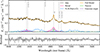Fig. 1.

Extracted quasar spectrum within a 0 $\overset{″}{.}$ $Mathematical equation: $ \overset{\prime \prime }{.} $$ 35 aperture centered on the spaxel with the highest integrated flux. The observed spectrum, shown in black, is aptly fit by the PyQSOFit model, shown in orange. Broad Hβ and Hγ are modelled using three and two broad Gaussian components (pink lines, individual Gaussians are shown in purple) with FWHM > 1200 km/s, and one Gaussian component with FWHM < 1200 km/s to trace narrow components (green line). The [O III] λλ4959,5007 emission lines are modelled with one broad and one narrow component. No narrow [O III] λλ4959,5007 components are detected, whereas a strong contribution from Fe II emission (blue line) is evident (Park et al. 2022). The lower panel shows fit residuals.

To analyze the spectrum, we used the public software PyQSOFit (Guo et al. 2018; Shen et al. 2019; Ren et al. 2024). We selected featureless spectral regions (4000–4200 Å, 4500–4700 Å, and 5050–5750 Å) to fit the quasar continuum. Our setup uses a power-law, a rest-frame optical Fe II template (Park et al. 2022) covering the Hβλ4861 (Hβ) region and an additional smooth second-order polynomial correction term to adjust the tilt and curvature of the fit. We fixed the redshift of the quasar at z = 7.6423 (as measured from [C II] λ157.6 μm by Wang et al. 2021). After subtracting the best-fit pseudo-continuum, we fit the Hβ emission line with three broad Gaussians (FWHM > 1200 km s⁻¹), as well as one narrow Gaussian (FWHM < 1200 km s⁻¹). The Akaike (AIC) and Bayesian (BIC) information criteria both indicate that a three-component broad Hβ model is ideal. Adding additional components does not significantly improve the χ², while a two-component model underfits the line profile. We fit Hγλ4340 (Hγ) with two broad and one narrow component. The [O III] λ4959 and [O III] λ5007 lines are fit with one broad and one narrow Gaussian each. In all fits, the flux ratios of the [O III] λλ4959,5007 doublet were constrained to their theoretical values, F₅₀₀₇/F₄₉₅₉ = 2.98 (e.g., Storey & Zeippen 2000). In our fit, the narrow core of the [O III] λλ4959,5007 lines collapsed to zero flux. Very weak wings were detected for the [O III] λλ4959,5007 lines (EW([O III] λ5007≈ 0.02 Å); however, this measurement is sensitive to the continuum placement and to the adopted decomposition of the Hβ base. Thus, we treated the [O III] λλ4959,5007 as not significantly detected and quote a 3σ upper limit on the EW of [O III] λ5007 measured from the local continuum noise, assuming a Gaussian line profile with a fixed full width at half maximum (FWHM) of 19 Å: EW([O III] λ5007) < 1.42 Å (based on the width of the detected narrow Hβ component). The broad-line Balmer decrement shows no evidence for BLR reddening. The resulting best-fit spectrum, along with the fits for the broad emission lines and the Fe II model components, is presented in Fig. 1.

3.2. Black hole mass and Eddington rate

Our best-fit broad Gaussian Hβ model (i.e., excluding the narrow component) has an FWHM of 4156 ± 68 km s⁻¹, which we interpret as virial broadening in the BLR (e.g., Peterson 2006). The instrumental broadening of the NIRSpec G395M/F290LP configuration is negligible compared to the measured broad Hβ width. Its error is dominated by the statistical uncertainty; we therefore do not apply an instrumental broadening correction. We measured the best-fit continuum monochromatic luminosity at rest-frame 5100 Å. To account for systematics, we added a conservative 10% flux calibration uncertainty in quadrature to the small statistical error⁴, obtaining L₅₁₀₀ = (1.77 ± 0.18)×10⁴⁶ erg s⁻¹. Together with the measured Hβ line width, this allows us to estimate the black hole mass M_BH of the central SMBH using single-epoch calibrations, such as Greene & Ho (e.g., 2005); Vestergaard & Peterson (e.g., 2006); Shen et al. (e.g., 2024), following Kaspi et al. (2000). We used the parametrization from Shen et al. (2024):

$\begin{matrix} log (\frac{M_{BH}}{M_{⊙}}) = 0.85 + 0.50 log (\frac{L_{5100}}{10^{44} erg s^{- 1}}) + 2.0 log (\frac{{FWHM}_{H β}}{km s^{- 1}}), \end{matrix}$ $Mathematical equation: $$ \begin{aligned} \log \left( \frac{M_{\rm BH}}{M_\odot } \right) = 0.85 + 0.50 \,\log \!\left( \frac{L_{5100}}{10^{44}\,\mathrm {erg\,s}^{-1}} \right) + 2.0 \,\log \!\left( \frac{\mathrm{FWHM} _{\rm H\beta }}{\mathrm{km\,s ^{-1}}} \right), \end{aligned} $$$ (1)

with an intrinsic scatter of σ_int = 0.45 ± 0.04 dex.

We obtained an Hβ single-epoch mass of M_BH, Hβ = (1.63 ± 0.10)×10⁹ M_⊙, and $M_{BH, H β} = (1 . 63_{- 1.05}^{+ 2.97}) \times 10^{9} M_{⊙}$ $Mathematical equation: $ M_{\mathrm{BH,H\beta}} = (1.63^{+2.97}_{-1.05}) \times 10^{9}\,M_\odot $$ when accounting for the intrinsic scatter. We used the measurements of Mg IIλ2800 and L₃₀₀₀ reported by Wang et al. (2021) to revisit the black hole mass estimate using the Mg IIλ2800 single-epoch calibration of Shen et al. (2024), yielding M_BH,Mg II = (3.18 ± 1.06) × 10⁹ M_⊙; or $M_{BH, Mg I I} = (3 . 18_{- 2.11}^{+ 6.26}) \times 10^{9} M_{⊙}$ $Mathematical equation: $ M_{\mathrm{BH},{\mathrm{Mg}{\small { {\text{ II}}}}}} = (3.18^{+6.26}_{-2.11}) \times 10^{9}\,M_\odot $$ when including intrinsic scatter. Considering measurement uncertainties alone, the two estimates differ at the ∼1.8σ level. When the intrinsic scatter of the calibrations is included, the results are fully consistent. We note that using the Shen et al. (2024) calibration for the Mg IIλ2800-based black hole mass yields values that are higher by a factor of ∼2 compared to those obtained with the Vestergaard & Osmer (2009) calibration adopted by Wang et al. (2021) and Yang et al. (2021); the two estimates are consistent only when accounting for the intrinsic scatter of the relations.

We calculated the Eddington rate, λ_Edd, defined as the ratio of bolometric luminosity, L_bol, and the Eddington luminosity, $L_{Edd} = \frac{4 π G M_{BH} m_{p} c}{σ_{T}}$ $Mathematical equation: $ L_{\mathrm{Edd}} = \frac{4 \pi G M_{\mathrm{BH}} m_p c}{\sigma_T} $$ , where m_p is the proton mass, c is the speed of light, and σ_T is the Thomson scattering cross-section. We derived the bolometric luminosity using the bolometric correction factor from Richards et al. (2006), applying L_bol = 9.26 × L₅₁₀₀, which yields (1.64 ± 0.16)×10⁴⁷ erg s⁻¹. From our derived M_BH estimate, we calculated an Eddington ratio of λ_Edd = 0.80 ± 0.05 accounting only for measurement uncertainties. These findings corroborate the results of Wang et al. (2021), indicating that quasar J0313–1806 harbours a relatively mature SMBH accreting at a high Eddington rate. The results of the spectral fit are summarized in Table 1.

Table 1.

Results of spectral fitting for J0313–1806.

4. Extended nebular emission

4.1. Point spread function modeling

To identify any potential extended gas components linked to the host galaxy, outflows, or field sources in the cube, we must first model and subtract the unresolved light from the significantly more luminous central quasar. Here, we created an empirical model of the PSF based on the observations of the associated PSF star, TYC 5875-488-1. To precisely align the quasar and PSF star images, we first computed the 2D cross-correlation between the quasar and PSF star white-light images obtained by integrating the cubes over the wavelength range 3.5–5.1 μm. This cross-correlation evaluates the similarity between the images at different pixel offsets.

We applied a PSF alignment shift between the brightest spaxels of the collapsed cubes, determining a sub-pixel shift in Fourier space (e.g., Stone et al. 2001; Foroosh et al. 2002). This technique involves computing the Fourier transform of each wavelength slice, applying the calculated phase shift for sub-pixel precision, and then performing an inverse Fourier transform on the shifted data. We obtained x-shift = 1.48 pixels and y-shift = − 2.34 pixels. The aligned PSF star cube was computed as

$\begin{matrix} {\tilde{I}}_{PSF} (x, y) = F^{- 1} {F [I_{PSF} (x, y)] \cdot e^{- 2 π i (x_{shift}, y_{shift})}} . \end{matrix}$ $Mathematical equation: $$ \begin{aligned} \tilde{I}_{\text{PSF}}(x, y) = \mathcal{F} ^{-1} \left\{ \mathcal{F} [I_{\text{PSF}}(x, y)] \cdot e^{-2\pi i (x_{\text{shift}}, y_{\text{shift}})} \right\} . \end{aligned} $$$ (2)

To account for differences in the spectral energy distribution (SED) between the quasar and the PSF star, we extracted the integrated spectra using a circular aperture (radius = 7 pixels, i.e., 0 $\overset{″}{.}$ $Mathematical equation: $ \overset{\prime \prime }{.} $$ 35). The aperture scale is determined based on the analysis shown in Appendix B. At the chosen radius, the enclosed flux fraction is already within ≈1–2% of that measured with larger apertures and its wavelength dependence is smooth and consistent with the expected chromatic broadening of the JWST PSF. This indicates that the extracted flux is dominated by unresolved quasar light, with no evidence for a significant contribution from extended host emission.

The raw scaling factor per wavelength is given by S(λ) = F_quasar(λ)/F_PSF(λ). However, any small-scale fluctuations in S(λ) can introduce systematic artifacts in the residual spectrum. To mitigate this, we apply a Gaussian smoothing filter with σ = 5 pix along the spectral axis. The spectra and the smoothed wavelength-dependent scale factor are shown in the left panel of Fig. 2. The figure in the right panel shows that the PSF model (i.e., the smoothed and scaled PSF star) accurately traces the flux profile of the quasar.

Fig. 2.

PSF model. Left: Spectral comparison between the quasar and PSF star used to derive the PSF scaling factor. The extracted 1D spectra from the quasar (black) and PSF star (blue) were obtained using a circular aperture with radius 0 $\overset{″}{.}$ $Mathematical equation: $ \overset{\prime \prime }{.} $$ 35. The PSF spectrum is scaled down by a factor of 500 for visual comparison. While the PSF star shows a smooth stellar continuum, the quasar exhibits a prominent broad Hβ emission line and strong Fe II features. The wavelength-dependent scaling factor S(λ) computed as the ratio between the quasar and PSF spectra is shown in green. The scaling factor is smoothed with a Gaussian kernel of width σ = 5 pix before being applied slice by slice to the aligned PSF cube. Right: Median radial profiles extracted from the quasar cube (black dashed), the raw PSF star cube (orange), and the PSF star cube, corrected with the wavelength-dependent scaling factor (blue). The radial profiles are measured from the brightest pixel in white light of each cube. The colour-shaded areas correspond to the median absolute deviations of the quasar radial profile (grey) and the scaled PSF star cube (blue).

Once the smoothed scale factors were computed, we could apply them to each wavelength slice of the PSF star cube, scaling it to match the quasar SED as

$\begin{matrix} I_{PSF, scaled} (x, y, λ) = S_{smooth} (λ) \times {\tilde{I}}_{PSF} (x, y, λ), \end{matrix}$ $Mathematical equation: $$ \begin{aligned} I_{\text{PSF,} \text{ scaled}}(x, y, \lambda ) = S_{\text{smooth}}(\lambda ) \times \tilde{I}_{\text{PSF}}(x, y, \lambda ), \end{aligned} $$$ (3)

where S_smooth(λ) denotes the smoothed wavelength-dependent scale factor, and ${\tilde{I}}_{PSF} (x, y, λ)$ $Mathematical equation: $ \tilde{I}_{\text{PSF}}(x, y, \lambda ) $$ is the subpixel-aligned PSF cube.

The final PSF-subtracted quasar cube is then obtained by subtracting the scaled PSF cube from the observed quasar data,

$\begin{matrix} I_{residual} (x, y, λ) = I_{quasar} (x, y, λ) - I_{PSF, scaled} (x, y, λ) . \end{matrix}$ $Mathematical equation: $$ \begin{aligned} I_{\text{residual}}(x, y, \lambda ) = I_{\text{quasar}}(x, y, \lambda ) - I_{\text{PSF,} \text{ scaled}}(x, y, \lambda ). \end{aligned} $$$ (4)

The resulting residual cube I_residual(x,y,λ) reveals the underlying spatially extended emission that is not associated with the unresolved quasar core. This emission can originate from NLRs, the host galaxy, outflows, satellite companions, or chance-aligned field fore- or background sources. A visual overview of the PSF subtraction process is presented in Fig. 3.

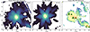Fig. 3.

PSF subtraction procedure for J0313–1806. Left: Integrated white-light image of the reduced cube centered on J0313–1806. The blue cross marks the position of the unresolved quasar. Center: Integrated and scaled cube of the PSF calibration star TYC 5875-488-1, aligned and scaled to match the quasar emission. The orange cross marks the position of the unresolved star. Right: Residual white-light image of J0313–1806 after PSF subtraction, revealing extended emission components after removal of the unresolved quasar core. We highlight three regions of interest: (A) A bright core near the quasar, (B) a near-elliptical diffuse region just northeast of the quasar, and (C) a distinct foreground elliptical source to the southwest of the quasar. This work focuses on the central region (A). For all maps, pixels with negative integrated flux were masked.

Despite the careful modeling and subtraction procedure, several sources of systematic uncertainty remain. First, the SEDs of the quasar and the PSF star differ intrinsically, introducing wavelength-dependent mismatches that are not fully corrected by the smooth scaling procedure. Second, subpixel alignment errors, particularly in the presence of asymmetric PSF wings or optical distortions, can leave residual artifacts in the final cube. We have assessed the impact of these effects through a series of robustness tests. Varying the degree of spectral smoothing applied to the scaling factor S(λ) results in negligible changes to the residual maps and does not affect the detection of extended emission. In addition, perturbing the relative alignment between the quasar and PSF star cubes at the level of the measured alignment uncertainty produces only minor changes in the residual root-mean-square (RMS). Residual artifacts associated with these systematics are confined to the central PSF core and do not generate spatially extended or spectrally coherent features. Therefore, we conclude that these systematic uncertainties do not affect the results or interpretations presented below.

In the collapsed PSF-subtracted cube, we identified three regions of interest. A luminous core close to the quasar position at pixel (50,45), shown as a green cross close to A; the object of the present paper. We further identified an extended quasi-elliptical, nebulous region to the north-east (B) of the quasar. The origin of this emission is further discussed in Appendix C. We also found a distinct source to the south-west (C) is spatially co-incident with a foreground galaxy detected in JWST/Near Infrared Camera (NIRCam) and JWST/Mid-Infrared Instrument (MIRI) imaging from the same Cycle 1 programme (#1764). The extracted source has photometry consistent with that of a galaxy at z ∼ 2.25 (Pudoka et al. 2025, and private communication). A clear detection in the F090W filter consolidates the lower redshift nature of this source. A spectrum extracted at this location displays a strong emission line, fixing the galaxy to z = 2.30, through its Paβλ12818 line. In Appendix D, we present spectra extracted within 0 $\overset{″}{.}$ $Mathematical equation: $ \overset{\prime \prime }{.} $$ 35 of the emission regions A, B, and C. The alternating horizontal pattern near region A is a PSF subtraction artifact caused by residual structured PSF wings (including diffraction features) and IFU sampling.

4.2. Balmer kinematic moment maps

After the PSF subtraction, we fit the data cube with a combination of host continuum and emission line models using the cube analysis software package q3dfit⁵ (Rupke 2014; Rupke et al. 2021), operating in fitpoly mode. We applied Gaussian smoothing with a 2.5 pixel (∼0.5 kpc) kernel along the spatial dimensions to suppress pixel-to-pixel noise fluctuations and enhance the detectability of low–surface-brightness emission, while also mitigating aliasing effects. The continuum was modeled with a third-order polynomial, while emission lines were fitted with single Gaussian components. Initially, we restricted the line fitting to [O III] λ5007 and the Balmer lines Hβ and Hγ, with the Balmer lines kinematically tied. We stress that [O III] λ5007 and the Balmer lines are fitted individually, allowing the code to trace kinematically distinct regions. Prior to fitting, the model spectra were convolved to match the spectral resolution of the G395M grating. We allow the code to fit lines up to σ = 2500 km s⁻¹ (FWHM ≈ 5900 km/s), a permissive upper bound for extended ionized gas around a quasar. We obtain zeroth-, first-, and second-order kinematic moments using q3dfit. The flux map was obtained from the single-Gaussian line fits. No spaxel with [O III] λλ4959,5007 (S/N > 3 in flux) was detected. While we cannot exclude that this is an artifact of the PSF subtraction procedure, we treated [O III] λλ4959,5007 as non-detected. For Hβ, we applied a signal-to-noise threshold of S/N_Hβ > 3 on the zeroth moment maps. Adjunct spaxels in eight-connectivity to these detected spaxels with at least S/N_Hβ > 1.5 were also conserved for plotting purposes only. The moment maps are displayed in Fig. 4. Pixels not fulfilling this criterion were masked. Overall, the Hβ emission region forms an envelope or shell-like structure centered on the quasar. A total of 57 spaxels have robustly detected Hβ with S/N_Hβ > 3, extended over a region of radius of ∼1.79 kpc of the quasar position. We formally refer to this structure as the Hβ shell. We further identified 46 spaxels with 1.5 < S/N_Hβ < 3, which are in eight-connectivity to neighboring spaxels where Hβ is 3σ detected. Although it is kinematically tied to Hβ, Hγ was only detected in 11/57 of the S/N_Hβ > 3 spaxels at an integrated S/N_Hγ > 2. The average projected distance of these spaxels to the quasar is 1.06 kpc. The velocity offset is traced by the v₅₀ parameter (i.e., the shift in velocity space at 50% of the line intensity). We note that the detection of parts of the Hβ shell is also warranted with less aggressive spatial smoothing (e.g., a kernel of 1 pixel).

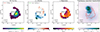Fig. 4.

Kinematic moment maps of Hβ around J0313-1806 and bandwidth-matched continuum. Gaussian spatial smoothing over a 2.5 pixel kernel was applied (at 0 $\overset{″}{.}$ $Mathematical equation: $ \overset{\prime \prime }{.} $$ 05/pix scale). First panel: Flux map of 3σ detected Hβ (57 spaxels). These are highlighted by the red contour. We define this distribution as Hβ shell. Adjunct spaxels in eight-connectivity to these detection spaxels with at least S/N_Hβ > 1.5 are also shown. The flux in the line peaks close to the quasar location, consistent with a central ionizing source. Second panel: Velocity offset map as traced by the the v₅₀ parameter. A clear velocity gradient is observed along the shell, indicating expansion or rotation of the structure. Spaxels with extreme velocities (∣v₅₀ ∣ > 400 km s⁻¹) are marked with green contours. Third panel: Velocity dispersion, σ. Patches of large dispersions (> 600 km/s) are observed at the edges and to the south-east of the structure, potentially indicating highly turbulent gas motion. Fourth panel: Continuum map constructed by integrating the fitted continuum model over a line-free spectral window with bandwidth matched to that of Hβ. While elevated continuum emission overlaps spatially with the Hβ shell, the absence of brightened nuclear morphology in the map following the Hβ flux confirms that the observed Hβ structure is not driven by background variations or continuum residuals. The continuum map shows a clear flux peak offset to the north from the quasar position. This component does not trace the shell-like Hβ morphology and lacks any associated kinematic structure. We therefore interpret it as an artifact from imperfect fitting in imperfectly PSF-subtracted spaxels, rather than extended stellar or nebular continuum emission.

We first observe that the total fitted line flux map of Hβ shows an arc-like shape with a flux maximum in the center of the shell at the pixel (50,45), near the unresolved quasar position (49,46), supporting the presence of a central ionizing source (i.e., the actual AGN or a nuclear central star cluster). The slight offset between the Hβ-flux peak and the quasar position is within the FWHM of the JWST PSF and is attributable to residual PSF subtraction effects. In Fig. 4, the v₅₀ map displays a clear velocity dipole from blueshifts to redshifts south-east to north-west. We measure a median blueshifted (v₅₀ < 0 km s⁻¹) velocity $v_{50, blue} = - 113_{- 27}^{+ 17} {km s}^{- 1}$ $Mathematical equation: $ v_{\mathrm{50,blue}}= -113^{+17}_{-27}\,\mathrm{km\,s}^{-1} $$ and a median redshifted (v₅₀ > 0 km s⁻¹) velocity $v_{50, red} = 32_{- 8}^{+ 4} {km s}^{- 1}$ $Mathematical equation: $ v_{\mathrm{50,red}}= 32^{+4}_{-8}\,\mathrm{km\,s}^{-1} $$ . The gradient of the velocity field appears centered on the quasar. The offset values are typical of AGN outflows (e.g., Liu et al. 2024). The symmetric, ordered nature of the velocity field around the quasar indicates a coherent large-scale kinematic pattern, consistent with a tilted or partial expanding shell of ionized gas (e.g., Ishibashi et al. 2021), although other complex organized motions (e.g., rotation Ishikawa et al. 2025 or a biconical flow) cannot be excluded. The apparent arc-like geometry of the nebula might also be due to PSF-over-subtraction close to the quasar, effectively depleting signal in Hβ. For simplicity, we assumed a spherical shell-like geometry (i.e., a complete sphere around the quasar) while acknowledging that this might not fully capture the real structure of the ionized gas. Finally, the dispersion map shows strong velocity dispersions, with a median dispersion of σ = (415 ± 51) km s⁻¹. Such dispersions are typically associated with AGN outflows and turbulent gas motion (e.g., Wylezalek et al. 2022). Spaxels corresponding to extreme velocity offsets in the v₅₀ map, i.e., ∣ v₅₀ ∣ > 400 km s⁻¹ shown with green contours, appear to also correspond to the highest dispersions σ > 600 km s⁻¹. We note that we cannot fully exclude the possibility that the observed Hβ distribution is directly tracing the host galaxy of J0313−1806 or a merging companion. Deep rest-frame UV/optical imaging with JWST/NIRCam will be required in the future to investigate the presence of a possible co-spatial stellar continuum. In Fig. 4 the control continuum map is constructed by integrating the continuum model over a line-free spectral window with bandwidth matched to that of Hβ (three times the median velocity σ of Hβ), does not reproduce the peaked structure seen in the line emission, indicating that the observed structure is not driven by continuum or background systematics.

Considering only the 57 spaxels with at least a 3σ detection of Hβ, we constructed a mean stacked spectrum of the shell shown in Fig. 5. The Hβ line is clearly detected, while [O III] λ5007 remains undetected, and with a median S/N_Hγ = 1.44, Hγ is not detected. We also show the mean stacked spectra, split by their v₅₀ values, to highlight differences in the Hβ line profile between blueshifted (v₅₀ < −25 km s⁻¹) and redshifted (v₅₀ > 25 km s⁻¹) regions of the Hβ shell. The blueshifted spaxels exhibit a slightly higher continuum and weaker emission lines compared to the redshifted ones. We compute the integrated 3σ upper limit on [O III] λ5007 in the Hβ shell (57 spaxels with Hβ at S/N > 3) as

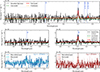Fig. 5.

Upper panel: Mean spectrum of the Balmer shell. This spectrum was extracted from 57 spaxels with at least 3σ Hβ detections. The line (green dashed line), the continuum (orange dashed line), and the full (red line) models are from our q3dfit analysis. The fitted, redshifted [O III] λ5007 and continuum emissions are consistent with noise. Middle panel: Zoom in spectra of the Hγ and Hβ regions. Lower panels: Mean spectra of blueshifted (v₅₀ < −25 km s⁻¹, left) and redshifted (v₅₀ > 25 km s⁻¹, right) Hβ spaxels.

$\begin{matrix} F_{[O III] < 3 σ} = 3 \sqrt{\sum σ_{i j, [O III]}^{2}}, \end{matrix}$ $Mathematical equation: $$ \begin{aligned} F_{{[{\text{ O}}{{\small { {\text{ III}}}}}]} < 3\sigma } = 3 \sqrt{\sum \sigma _{ij,{[{\text{ O}}{{\small { {\text{ III}}}}}]}}^2}, \end{aligned} $$$ (5)

where σ_ij,[O III] is the per-spaxel 1σ noise uncertainty in the spectrum at the location of [O III]. The corresponding integrated flux ratio upper limit is then

$\begin{matrix} {log}_{10} {(\frac{F ([O III])}{F (H β)})}_{< 3 σ} = {log}_{10} (\frac{F_{[O III] < 3 σ}}{\sum_{ij} F_{ij} (H β)}) = - 1.15, \end{matrix}$ $Mathematical equation: $$ \begin{aligned} \log _{10} \left( \frac{F({[{\text{ O}}{{\small { {\text{ III}}}}}]})}{F(\mathrm{H} \beta )} \right)_{<3\sigma } = \log _{10}\left( \frac{ F_{{[{\text{ O}}{{\small { {\text{ III}}}}}]} < 3\sigma }}{\sum _{ij} F_{ij}(\mathrm{H} \beta )} \right) = -1.15, \end{aligned} $$$ (6)

where F_ij(Hβ) is the spaxel-wise flux measured in the 3σ-detected Hβ line. The integrated flux of [O III] λ5007 in the extended ionized shell is thus lower than 10^−1.15 ∼ 7.1% of the integrated Hβ flux at the 3σ confidence level. Using the same methodology, we also measure the 3σ upper limit on the He IIλ1640 to Hβ ratio in the Hβ nebula. We obtain ${log}_{10} {(\frac{F ([He I I])}{F (H β)})}_{<, 3 σ} = - 1.15$ $Mathematical equation: $ \log_{10} \left( \frac{F({[{\mathrm{He}{\small { {\text{ II}}}}}]})}{F(\mathrm{H}\beta)} \right) _{ < ,3\sigma} = -1.15 $$ .

5. Discussion

We discuss the nuclear (Sect. 5.1) and kpc-scale (Sect. 5.2) properties derived for J0313−1806 separately. In Sect. 5.3, we discuss our interpretation of the results as evidence for episodic feedback cycles.

5.1. Suppressed nuclear [O III] emission

The nuclear quasar spectrum displays a broad Hβ line and strong Fe II emission, whereas [O III] λλ4959,5007 emission is absent (Fig. 1). Weak or absent [O III] λλ4959,5007 emission is not uncommon in quasar samples across cosmic time (e.g., Netzer et al. 2004). In the following, we discuss similar objects in the literature and possible physical origins for the lack of [O III] λλ4959,5007 in J0313–1806.

5.1.1. A possible high-z weak line quasar

Weak-line quasars (WLQs) are AGNs with absent or very low-EW broad UV emission lines, most prominently, the high-ionization lines (e.g., C IVλ1549, He IIλ1640). The resonant low-ionization line Lyαλ1216 is often also weak, and mid-ionization lines (e.g., C III] λ1909], Si III] λ1892]) are frequently damped (Fan et al. 1999; Diamond-Stanic et al. 2009; Shemmer et al. 2010; Plotkin et al. 2015; Chen et al. 2024). The number density of WLQs appears to increase with redshift, with a fraction of roughly 10 − 15% at z ∼ 6 (Bañados et al. 2016; Shen et al. 2019), compared to 1.3% in the Sloan Digital Sky Survey (SDSS; York et al. 2000) at z ≲ 4.2 (Diamond-Stanic et al. 2009).

Broad UV high-ionization line measurements for J0313–1806, in particular C IVλ1549, have already been presented by Yang et al. (2021). They report a C IVλ1549 rest-frame EW = 14.2 ± 0.9 Å and a blueshift of C IVλ1549 relative to the systemic redshift from [C II] λ157.6 μm of Δ v_{C IV−[C II]} = −4138 ± 350 km s⁻¹. This makes the line slightly stronger than the canonical EW < 10 Å criterion used to define WLQs by Diamond-Stanic et al. (2009), see also Shemmer et al. (2010), Wu et al. (2011), Luo et al. (2015), Plotkin et al. (2015), Chen et al. (2024), but consistent with the EW < 15 Å criterion adopted by Ni et al. (2018), Timlin et al. (2020). J0313−1806 thus lies at the boundary of commonly adopted WLQ definitions and could be considered a weak-line quasar under the more inclusive criterion.

The combined C IVλ1549 EW and strong blueshift of J0313–1806 are consistent with those of WLQs (see Fig. 2 of Ni et al. 2018 and Fig. 9 of Timlin et al. 2020), and are well offset from the locus of typical quasars. To quantify this behavior in a way that reduces the degeneracy between C IVλ1549 EW and blueshift, we adopt the C IV ∣∣ Distance metric (Rivera et al. 2020, 2022, computed following Ha et al. 2023). This metric combines the two observables into a single scalar quantity that measures how far a source lies along the empirical C IVλ1549 sequence defined by the quasar population, with larger values corresponding to more extreme C IVλ1549 properties. The resulting the C IV ∣∣ Distance for J0313–1806 is ≃1.10. At the independently measured Hβ-based accretion rate of L_bol/L_Edd = 0.80 ± 0.05, this value is consistent with the locus occupied by WLQs in the C IV∣∣Distance–L_bol/L_Edd plane (Ha et al. 2023), supporting the classification of J0313–1806 as WLQ-like.

We measured the rest-frame EWs of Hβ and the Fe II in the 4434–4684 Å spectral window from the quasar spectrum extracted in Section 3.1. The EW of the fitted broad [O III] λλ4959,5007 wings is extremely small (≈0.02 Å) and we thus obtained a conservative 3σ upper limit for the EW of [O III] λ5007 in the spectral window 4988–5028 Å. We obtain EW(Hβ) = 53.18± 0.31 Å, EW(Fe II) = 38.46± 0.02 Å and EW([O III] λ5007) < 1.42 Å (see Table 1) and compare these values to the WLQ sample of Chen et al. (2024), as well as to a control sample of typical SDSS quasars (135 738 quasars with EW(Hβ) and EW([O III]) values from data release 16, DR16Q, Lyke et al. 2020; Wu & Shen 2022) in Fig. 6. The [O III] λλ4959,5007 emission in J0313–1806 is particularly weak relative to its Hβ emission, even when compared to typical WLQs.

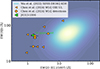Fig. 6.

EWs of Hβ and upper limit on [O III] λ5007 for J0313-1806 (green triangle). We compare it to a sample of WLQs identified by Chen et al. (2024) (orange circles for detected [O III] λ5007, orange triangles for upper limits). We also show Gaussian kernel density contours for SDSS DR16Q quasars (Wu & Shen 2022). This highlights the particular weakness of the [O III] λλ4959,5007 emission in the nuclear spectrum of J0313–1806, even relative to typical WLQs.

The physical driver of the UV-line weakness in WLQs remains debated. One possibility is that the BLR is said to be anemic due to its low gas content and/or covering factor (Shemmer et al. 2010). Alternatively, a soft ionizing continuum could also produce weak high-ionization emission lines. Investigating a sample of seven WLQs, Plotkin et al. (2015) find that their rest-frame optical low-ionization lines (e.g., Hβ) are not as exceptionally weak as their UV lines. These findings favor the soft-ionizing-continuum scenario, since an anemic BLR would result in all broad lines being similarly weak.

Plotkin et al. (2015) further report typical Hβ widths with FWHM < 4000 km s⁻¹, strong Fe II emission, and large C IVλ1549 blueshifts (up to 5500 km s⁻¹). As many as ∼50% of all WLQs are X-ray weak (e.g., Wu et al. 2011; Luo et al. 2015; Ni et al. 2018, 2022; Pu et al. 2020) relative to typical rest-frame UV-to-X-ray ratios in Type 1 AGN (Steffen et al. 2006). The hard X-ray spectra of X-ray weak WLQs (typical photon index range, Γ ∼ 1.1–1.2; Luo et al. 2015; Pu et al. 2020) support the idea that absorption and Compton-thick shielding play an important role for the line emission in WLQs (see also Ni et al. 2022).

In the high- or super-Eddington accretion regime, the accretion disk becomes geometrically thick (Abramowicz et al. 1988, see also Abramowicz 2005 and references therein). Once puffed up, the disk can shield the BLR from hard ionizing radiation, resulting in an overall soft SED (Wang et al. 2014; Madau & Haardt 2024; Lupi et al. 2024b). This shielding can explain both the absence of high-ionization lines in WLQs and their observed X-ray weakness. Additionally, the large C IVλ1549 blueshifts observed in WLQ samples (Luo et al. 2015; Plotkin et al. 2015) are consistent with the presence of powerful line-driven winds expected in high or super-Eddington disks (Castor et al. 1975; Murray et al. 1995). Another recurring feature is the weakness of [O III] λλ4959,5007 emission observed in WLQ samples (Leighly et al. 2007; Shemmer et al. 2010; Wu et al. 2011; Plotkin et al. 2015; Ha et al. 2023; Eilers et al. 2023; Chen et al. 2024). In the puffed-up high-L/L_Edd scenario, the shielding of > 35 eV photons can also naturally explain the absence of [O III] λλ4959,5007 lines in WLQ spectra. The anti-correlation between the strength of [O III] λλ4959,5007 emission and the accretion rate has long been studied in the Eigenvector 1 context (EV1, e.g., Boroson & Green 1992; Sulentic et al. 2000; Marziani et al. 2001; Shen & Ho 2014; Wolf et al. 2020). In addition, the Baldwin effect (Baldwin 1977; Zhang et al. 2013; Stern & Laor 2013; Shen & Ho 2014) describes the general decrease in the EW of emission lines, including [O III] λλ4959,5007, with increasing quasar luminosity. Indeed, weak or absent [O III] λλ4959,5007 emission has also been observed in targeted luminous quasar samples, such as the WISE/SDSS-selected hyper-luminous (WISSH) quasar survey (Vietri et al. 2018), which probes the most extreme end of the quasar luminosity function. Vietri et al. (2018) argue that the relative [O III] λλ4959,5007 weakness observed in ∼70% of their sample is mainly driven by orientation effects. The NLR is photoionized within the polar ionization cone. When viewed more face-on, i.e., looking down the cone, the bright continuum outshines the projected NLR emission, resulting in a higher continuum-to-NLR ratio than in more edge-on orientations. In addition to high L/L_Edd and orientation effects, obscuration by dust or dense gas has also been invoked to explain reduced [O III] λλ4959,5007 emission in quasars (Temple et al. 2019; Wang et al. 2025).

Another well-known class of fast accretors that display weak [O III] λλ4959,5007 emission are narrow-line Seyfert 1 galaxies (NLSy1; Osterbrock & Pogge 1985; Goodrich 1989). However, we note that these objects are strictly classified based on their narrower Hβ profiles (< 2000 km s⁻¹), a criterion that is not met by J0313–1806.

5.1.2. J0313–1806 and the quasar main sequence

In addition to sharing characteristic WLQ properties, J0313–1806 is also a BAL quasar, indicative of strong outflows and/or shielding on nuclear scales. Such BAL features are extremely rare among WLQs (e.g., Nikołajuk & Walter 2012), with one other case reported by Yi et al. (2019). To anchor J0313–1806 in the EV1 context, we place it along the quasar main sequence (see, e.g., Marziani et al. 2018, for a review), in the primary EV1 plane defined by the FWHM of Hβ and the relative strength of the optical Fe II emission, quantified as r_Fe II = F(Fe II)/F(Hβ). For J0313–1806, we had obtained FWHM(Hβ) = 4156 ± 68 km s⁻¹ and compute r_Fe II = 0.95± 0.13. Archetypal quasar categories have been defined along this sequence (Sulentic et al. 2000), thought to be primarily driven by a combination of accretion rate (L/L_Edd) and the viewing angle toward a flattened BLR (e.g., Shen & Ho 2014). A canonical boundary at FWHM(Hβ)≃4000 km s⁻¹ separates rapidly accreting sources (Population A, FWHM(Hβ)≲4000 km s⁻¹) from more massive, lower-accretion systems (Population B, FWHM(Hβ)≳4000 km s⁻¹, e.g., Marziani et al. 2001). WLQs typically occupy the extreme Population A (xA) regime, characterized by r_Fe II ≳ 1 (Diamond-Stanic et al. 2009; Martínez-Aldama et al. 2018; Dultzin et al. 2020).

In Fig. 7, we show the distribution of SDSS DR16Q quasars (Lyke et al. 2020; Wu & Shen 2022) in the redshift range 0.4 < z < 0.8, selected following Shen & Ho (2014) with the criteria 0 < r_Fe II < 3, uni_flag≠0, 800 km s⁻¹ < FWHM(Hβ) < 15 000 km s⁻¹, and sn_flag > 10. The colour scale indicates the mean log₁₀ EW([O III]) in bins of Δ r_Fe II = 0.1 and ΔFWHM(Hβ) = 500 km s⁻¹. We mark the position of J0313–1806 and overlay the WLQs presented by Chen et al. (2024), colour-coded by their measured or upper-limit EW([O III]). J0313–1806 lies at the edge of the xA regime (formally r_Fe II > 1). Several WLQs from Chen et al. (2024) also occupy a similar region of the plane. Notably, several of these objects exhibit EW([O III] λ5007) values or limits that fall far below the typical SDSS DR16Q quasars in their local EV1 bins.

Fig. 7.

EV1 plane FWHM(Hβ) vs. r_Fe II. The distribution of a subset of SDSS DR16Q quasars from Wu & Shen (2022) is shown in black (see text for selection criteria). The colourmap gives the mean log₁₀EW([O III]) in bins of size Δ r_Fe II = 0.1 and ΔFWHM(Hβ) = 500 km s⁻¹. J0313-1806 is shown as a green star. WLQs from Chen et al. (2024) are shown as circles (measured EW([O III] λ5007)) or triangles (upper limits), colour-coded according to their log₁₀EW([O III]). J0313–1806 and several WLQs lie outside the xA regime (r_Fe II > 1) but nonetheless show strikingly weak [O III] λ5007 emission compared to SDSS DR16Q quasars in the same EV1 bins.

Quantitatively, the 3σ upper limit on EW([O III] λ5007) for J0313–1806 is a factor of ∼37 lower than the median value of SDSS DR16Q quasars at the same EV1 location (EW([O III]) = 15.76 Å), bin 0.90 ≤ r_Fe II < 1.00 and 3800 ≤ FWHM(Hβ) < 4300 km s⁻¹, containing 369 sources). This deficit corresponds to a one-sided percentile of p = 3.8 × 10⁻⁷, namely, a 4.95σ outlier with respect to the local quasar population.

J0313–1806 exhibits exceptionally weak nuclear [O III] λ5007 emission compared to both the general quasar population at the same EV1 location and to local WLQs. This suggests that the extreme weakness of [O III] λλ4959,5007 in J0313–1806 cannot be attributed solely to high- or super-Eddington accretion, but likely requires additional factors such as orientation, obscuration, or collisional de-excitation. In the paradigm presented by Shen & Ho (2014), at a fixed r_Fe II, the spread in FWHM(Hβ) primarily reflects orientation effects, with broader FWHM(Hβ) corresponding to more edge-on viewing angles and narrower profiles to more face-on systems. For J0313−1806, our measured FWHM(Hβ) and r_Fe II place it among the broader Hβ profile sources at this r_Fe II (see black dots in Fig. 7), suggesting more edge-on configurations. Consequently, orientation alone is also unlikely to explain the unusually weak [O III] λλ4959,5007 emission.

5.2. Suppressed extended [O III] emission

To further constrain the scenarios responsible for weak [O III] λλ4959,5007 in J0313–1806, we to on to discuss the kpc-scaled Hβ emitting shell illuminated around the nucleus revealed in our JWST/NIRSpec IFU observation.

5.2.1. Photoionization simulations

In AGN, narrow-line emission can be observed out to kpc scales around the central continuum source (e.g., Bennert et al. 2002; Schmitt et al. 2003; Greene et al. 2011; Hainline et al. 2014; Liu et al. 2014). In quasar NLRs typical densities reach n_e ∼ 10^2 − 4 cm⁻³ (e.g., Bennert et al. 2006; Nagao et al. 2006; Kakkad et al. 2018; Joh et al. 2021), allowing forbidden high-ionization lines such as [O III] λλ4959,5007 to be efficiently produced in partially ionized gas. This is not the picture observed in the extended emission around J0313–1806, where we report broadened Hβ emission, with a median velocity dispersion of σ = (415 ± 51) km s⁻¹ but no significant [O III] λλ4959,5007 in the immediate kpc-scale environment of the quasar. The observed peak in the Hβ flux distribution suggests that the ionized shell is illuminated by the central source. The absence of [O III] λλ4959,5007 emission throughout the shell is intriguing, and we explore potential physical scenarios to explain this in light of the simultaneous lack of nuclear [O III] λλ4959,5007 emission (Sect. 5.1).

One of the leading physical explanations for the absence of [O III] λλ4959,5007 in luminous quasars, as discussed in Section 5.1.2, is an orientation effect: the BLR outshines the NLR along low-inclination sightlines (e.g., Vietri et al. 2018). However, the complete absence of extended [O III] λλ4959,5007 emission in the PSF-subtracted NIRSpec/IFU cube disfavors this interpretation for the shell. The extended and nuclear [O III] λλ4959,5007 weakness must therefore be explained by the physical state of the gas and/or the ionizing SED rather than by orientation alone.

We carry out simulations with the python front-end PYCLOUDY (v0.9.15; Morisset 2013) and the CLOUDY photoionization code c23.01 (Ferland et al. 2013; Gunasekera et al. 2023), which computes the thermal, ionization, and line-emission structure of the shells.

Since Hαλ6563, as well as the forbidden lines [N II] λ6583 and [S II] λλ6716,6731, lie outside the spectral window of our observations, and other diagnostic features such as the auroral [O III] λ4363 line are too faint to be detected, we cannot apply standard emission line ratio diagnostics (e.g., Baldwin et al. 1981; Veilleux & Osterbrock 1987; Kauffmann et al. 2003; Kewley et al. 2006; Mazzolari et al. 2024; Scholtz et al. 2025). We use two primary diagnostic ratios: log₁₀([O III] 5007/Hβ) and log₁₀([He II] 4686/Hβ). We model a spherical shell of photoionized gas extending from r_in ∈ {0.1, 0.8, 1.7} kpc to r_out = 1.8 kpc, with covering factor C_f = 0.9. The covering factor mimics an opening along our line of sight, exposing the BLR, as required by the observed nuclear broad Hβ. We note that varying C_f rescales the total line luminosities but leaves ratios unchanged to first order. The gas is dust-free, has constant density at the illuminated face, and is spherical (sphere). We vary metallicity over log(Z/Z_⊙)∈[−2.50, 0.25] in steps of 0.25 dex and density a wide range log n_H/cm⁻³ = {3−8} in steps of 0.5 dex. Metallicity-dependent elemental abundances are adopted following the analytic prescriptions of Nicholls et al. (2017, see also Decarli et al. 2024); in particular the oxygen abundance scales as

$\begin{matrix} 12 + log (O / H) = 8.76 + log Z, \end{matrix}$ $Mathematical equation: $$ \begin{aligned} 12 + \log (\mathrm{O} /\mathrm{H} ) \;=\; 8.76 + \log Z, \end{aligned} $$$ (7)

with log Z the logarithmic metallicity relative to solar. We bracket the possible ionizing spectral shapes with two parameterized AGN continua using CLOUDY’s agn command. The rest–UV spectral slope is fixed by the spectrum in Wang et al. (2021): α_λ ≃ −0.91 near Lyα, which implies α_ν = − (2 + α_λ) = − 1.09. We therefore kept α_uv = −1.09 in all models and vary only the high-energy shape of the SEDs. Our AGN normal continuum adopts T = 1.0 × 10⁵ K, α_uv = −1.09, α_x = −1.0 (Γ ≃ 2.0), and α_ox = −1.4, representative of luminous quasars with standard X-ray output relative to their optical emission (Steffen et al. 2006; Just et al. 2007; Lusso et al. 2010; Nanni et al. 2017; Vito et al. 2019a). The “AGN soft” (WLQ-like) continuum instead has T = 1.0 × 10⁵ K, α_uv = −1.09, α_x = −1.7, and α_ox = −2.2, mimicking an extremely X-ray–weak quasar similar to observed WLQs (e.g., Luo et al. 2015; Timlin et al. 2020). Both continua are normalized to the observed optical luminosity νL_ν(5100 Å) = 1.77 × 10⁴⁶ erg s⁻¹, as derived in Section 3.1. The source models are shown in Fig. 8. Line emissivities are extracted per zone and integrated to total line powers. The O⁺→O⁺⁺ ionization edge lies at 35.1 eV (354 Å); the suppression of photons above this threshold, like in our soft model, naturally reduces the production of O⁺⁺ and thus the strength of [O III] λλ4959,5007 emission. However, in harder ionizing spectra, photons beyond the ionization edge at 54.9 eV (O⁺⁺→O³⁺) further ionize oxygen, generating O³⁺ and depleting [O III] λλ4959,5007. In this work, we have aimed to test the net effect of the EUV-X-ray SEDs on the O⁺⁺ ion population with our two models.

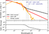Fig. 8.

AGN and stellar continuum models adopted in the CLOUDY simulations. Upper panel: AGN normal model with T = 1.0 × 10⁵ K, α_uv = −1.09, α_x = −1.0 (Γ ≃ 2.0), and α_ox = −1.4, representative of luminous quasars with typical X-ray emission, shown as a black line. The red line shows our AGN soft model with T = 1.0 × 10⁵ K, α_uv = −1.09, α_x = −1.7, and α_ox = −2.2, chosen to mimic the steeper and X-ray–weaker spectra representative of WLQs. The orange line shows the BPASS starburst model. The vertical dashed lines indicate the ionization thresholds for O⁺⁺ (35.1 eV) and O³⁺ (54.9 eV). Lower panel: Ratio of the two continua, highlighting that the AGN soft model strongly suppresses the hard ionizing photon budget compared to the AGN normal case.

Next, we set up a “nuclear star formation” ionizing source model using a BPASS v2.2.1 (Eldridge et al. 2017; Stanway & Eldridge 2018) spectrum corresponding to a 10 Myr instantaneous burst at solar metallicity (orange line in Fig. 8). The spectrum was normalized to a total ionizing photon output of log₁₀ Q(H)∼50, consistent with a vigorous nuclear starburst producing several × 10² M_⊙ yr⁻¹ (e.g., Kennicutt 1998) typical of luminous z ∼ 7 quasar hosts. We stress, however, that the quasar should overwhelmingly dominate the ionizing photon budget. Nuclear star-formation is included only as a comparison case to illustrate the ionization conditions expected in the absence of a hard AGN spectrum, rather than as a realistic alternative single power source.

In Fig. 9, we show the simulated line ratios log₁₀([O III] 5007/Hβ) across grids of the hydrogen density, n_H, and metallicity, Z, for the AGN normal,” “AGN soft,” and stellar models, each evaluated at three inner shell radii (r_in ∈ 0.1, 0.8, 1.7 kpc). Regions where log₁₀([O III]5007/Hβ) < −1.15 (Section 4.2) are highlighted as consistent with the ratio measured in the integrated spectrum of the shell. The illuminated skin of an AGN-irradiated shell is expected to be compressed until the gas pressure balances the incident radiation pressure, namely, the so-called radiation-pressure confinement (RPC; e.g., Draine 2011; Stern et al. 2014a,b; Baskin et al. 2014a,b; Baskin & Laor 2021). This sets a characteristic density floor, n_floor ∼ P_rad/(kT)≈L/(4πr²c kT). We did not enforce an RPC in our CLOUDY models; densities below this floor are shown for completeness but are treated as physically disfavoured. Figure 9 shows the corresponding “RPC exclusion zone.” Cosmological zoom-in simulations (Costa et al. 2015) indicate that cold gas can further be pressure-confined by a hot, volume-filling shocked medium (see also Stern et al. 2016). Even if this hot phase remains undetected in our IFU data, it would only add to the total pressure, so the RPC floor remains a valid lower bound.

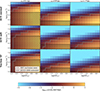Fig. 9.

Cloudy simulation results for the Hβ shell. Top and middle rows correspond to models using the AGN normal and AGN soft continua as ionizing sources, respectively, while the lower row corresponds to the stellar ionizing source. Each panel shows the predicted line ratio log₁₀([O III] 5007/Hβ) as a function of gas density, n_H, and metallicity, Z, for inner shell radii of r_in = 0.1, 0.8, and 1.7 kpc (left to right). The maps are spanned by constant-density shell models with outer radius r_out = 1.8 kpc. Regions enclosed by the black contour are consistent with the observed constraint log₁₀([O III]/Hβ) < −1.15 from the extended emission in J0313-1806. The hatched areas indicate the radiation–pressure confinement (RPC) exclusion zone, where densities fall below the expected RPC floor and are therefore disfavored.

We see only minor differences between the AGN normal and AGN soft continuum-driven runs in terms of the accessible parameter space, with slightly lower densities accessible in the AGN soft model. This indicates that, assuming AGN photoionization, the depletion of [O III] λλ4959,5007 is primarily driven by collisional de-excitation or metallicity rather than by spectral hardness. For all three inner radii probed, there exist regions of parameter space that are consistent with the observational constraint log₁₀([O III] 5007/Hβ) < −1.15, as well as regions that are inconsistent. To first order, our models show that reproducing the observed weakness of [O III] λλ4959,5007 requires either very high gas densities (n_H ≳ 10⁶ cm⁻³, where collisional suppression becomes efficient independent of metallicity) or, at lower densities (n_H ≲ 10⁵ cm⁻³), sub-solar metallicities (Z ≲ 0.2 Z_⊙). Thus, both high-density and low-metallicity solutions are supported.

At very high densities, n_H ≳ 10⁷ cm⁻³, collisional de-excitation is so efficient that the observed ratios can be reproduced almost irrespective of metallicity or shell thickness. At densities n_H ∼ 10^5 − 7 cm⁻³, the line ratios are increasingly suppressed with decreasing metallicity, Z ≲ 0.1–0.2 Z_⊙. For more moderate densities, n_H ≲ 10^4.5 cm⁻³, the predicted ratios exceed the observed limit across essentially the entire metallicity range. A thinner shell, namely, with a larger inner radius (e.g., r_in = 1.7 kpc), significantly relaxes the density requirements, enabling n_H ∼ 10⁵ cm⁻³. The even softer “nuclear star formation” SED enables access to consistent log₁₀([O III] 5007/Hβ) ratios over a larger set of density and metallicity combinations, with n_H ∼ 10⁴ cm⁻³ densities available up to log(Z/Z_⊙ ∼ 1).

We note, however, that even for the lower possible densities of n_H ≳ 10^3.5 cm⁻³, the total gas mass implied by a uniform, kpc-scale shell becomes unrealistically large. The ionized gas mass of a shell with inner radius, r_in, outer radius, r_out, covering factor C_f, and filling factor, f, is

$\begin{matrix} M_{gas} \approx 4 π C_{f} f μ m_{p} n_{H} (r_{out}^{3} - r_{in}^{3}) / 3, \end{matrix}$ $Mathematical equation: $$ \begin{aligned} M_{\rm gas} \;\approx \; 4\pi \, C_{\rm f}\, f\, \mu m_{\rm p}\, n_{\rm H}\, (r_{\rm out}^{3}-r_{\rm in}^{3})/3, \end{aligned} $$$ (8)

where μ ≃ 1.4 is the mean particle mass per hydrogen nucleus.

Considering the optimistic case of a thin shell with r_in ∼ 1.7 kpc, a shell thickness of 100 pc, C_f = 0.9, and n_H ∼ 10^3.5 cm⁻³, this expression yields M_gas ∼ 1.3 × 10¹¹ M_⊙ if the gas is volume-filling (i.e., f = 1). Such a mass is implausibly large for kpc-scale gas reservoirs in early galaxies. Compared to observational constraints from dust and [C II] λ157.6 μm (M_dust ∼ 7 × 10⁷ M_⊙, Wang et al. 2021) this would require unreasonably high gas-to-dust ratios (realistic gas-to-dust ratios are of the 10², e.g., Li et al. 2019). The dense phase required to collisionally quench [O III] λλ4959,5007 cannot be distributed in a volume-filling layer. Instead, the emitting material must occupy only a small fraction of the swept-up volume, implying a low filling factor (f ≲ 0.05) to keep the total ionized mass within reasonable bounds. One plausible realization is emission from dense clumps or a thin layer within the shell, but other geometries with similarly low filling factors cannot be excluded. We are assuming a spherical symmetric shell for simplicity, while the observed distribution is also consistent with a partial shell (or even more complex geometry), which would allow us to reduce the total gas mass by a factor of up to ∼10.

Our observed upper limit in [O III]/Hβ ratios is thus consistent with ionization from an AGN or nuclear star formation, only if we assume a clumpy geometry for the shell. In Section 4, we also derived an upper limit on a second line ratio: ${[{log}_{10} (\frac{F ([He I I])}{F (H β)})]}_{<, 3 σ} = - 1.12$ $Mathematical equation: $ \left[ \log_{10} \left( \frac{F({[{\mathrm{He}{\small { {\text{ II}}}}}]})}{F(\mathrm{H}\beta)} \right) \right]_{ < ,3\sigma} = -1.12 $$ . This ratio is primarily sensitive to the hardness of the ionizing radiation field and can be used to distinguish between AGN- and star formation–driven photoionization scenarios (e.g., Decarli et al. 2024). However, when comparing our 3σ upper limit to the simulation results presented by Decarli et al. (2024, see their Fig. 9), we find that our measurement does not allow us to conclusively differentiate between the two photoionization scenarios. However, we note that a soft ionizing continuum, such as that coming from a nuclear star-formation model, would significantly relax the density, thickness, and filling-factor requirements.

5.2.2. Hβ shell energetics

Following Osterbrock & Ferland (2006, see also Vayner et al. 2024; Liu et al. 2024), the recombination mass of the spatially resolved Hβ shell contained in each spaxel can be calculated as

$\begin{matrix} M_{ion}^{ij} = \frac{m_{p} L_{H β}^{ij}}{α_{H β} h ν_{H β} n_{e}}, \end{matrix}$ $Mathematical equation: $$ \begin{aligned} M_{\rm ion}^{ij} = \frac{m_p \; L_{\mathrm H\beta}^{ij}}{\alpha _{\mathrm H\beta} \; h\nu _{\mathrm H\beta} \, n_e}, \end{aligned} $$$ (9)

where m_p is the mass of the proton, L_Hβ the luminosity of Hβ, α_Hβ is the effective Hβ recombination coefficient, h is the Planck constant, ν_Hβ is the rest-frame frequency of Hβ, and n_e is the electron density. Here we assume that Hβ is mainly produced through recombination and model the emitting gas as an ensemble of identical, unresolved gas elements (hereafter referred to as clouds). Each cloud has a fixed electron density. Assuming Case B recombination, we calculated the recombination coefficient of Hβ using the nebular emission line analysis package pyneb (Luridiana et al. 2015). We note that the recombination mass is formally different than the total gas mass calculated in Eq. (9), as it only traces the H II region actively emitting Hβ.

We considered conditions similar to the ones supported by our Cloudy AGN simulations and set n_e = 10⁶ cm⁻³ (α_Hβ = 3.071 × 10⁻¹⁴ cm⁻³ s⁻¹) and fix the temperature to T = 10⁴ K. These numbers yield a total recombination mass of M_ion, tot = (1.02 ± 0.09)×10³ M_⊙ for the shell.

We then computed the integrated and instantaneous energetics of the outflow. We started with the integrated ionized mass outflow rate,

$\begin{matrix} {\dot{M}}_{ion}^{int} = \sum_{ij} \frac{M_{ion}^{ij} v_{out}^{ij}}{R^{ij}}, \end{matrix}$ $Mathematical equation: $$ \begin{aligned} \dot{M}_{\rm ion}^\mathrm{int} = \sum _{ij} \frac{M_{\rm ion}^{ij}\; v_\mathrm{out} ^{ij}}{R^{ij}}, \end{aligned} $$$ (10)

where v_out^ij = ∣v₅₀^ij ∣ +σ^ij is the outflow velocity, namely, the sum of the absolute velocity offset traced by the non-parametric v₅₀ and the velocity dispersion. This convention allows us to capture the maximum outflow velocity encoded in the winds of the emission line (Rupke & Veilleux 2013; Vayner et al. 2024). R^ij represents the physical projected distance between the spaxel (i, j) and the quasar coordinates (49,46). Following Vayner et al. (2024), we also obtained the spaxel-wise instantaneous mass outflow rate from

$\begin{matrix} {\dot{M}}_{ion}^{ij} = \frac{M_{ion}^{ij} v_{out}^{ij}}{d R}, \end{matrix}$ $Mathematical equation: $$ \begin{aligned} \dot{M}_{\rm ion}^{ij} = \frac{M_{\rm ion}^{ij}\; v_\mathrm{out} ^{ij}}{\mathrm{d} R}, \end{aligned} $$$ (11)

where dR is the physical size of a single spaxel. We further calculate integrated and instantaneous momentum and kinetic luminosities using

$\begin{matrix} \begin{matrix} {\dot{P}}_{ion}^{ij} & = M_{ion}^{ij} v^{ij}, E_{kin, ion}^{ij} = \frac{1}{2} M_{ion}^{ij} {(v^{ij})}^{2} . \end{matrix} \end{matrix}$ $Mathematical equation: $$ \begin{aligned} \begin{aligned} \dot{P}_{\mathrm{ion} }^{ij}&= M_{\mathrm{ion} }^{ij} \; v^{ij}, \qquad E_{\mathrm{kin,ion} }^{ij} = \frac{1}{2} M_{\mathrm{ion} }^{ij} \; (v^{ij})^2. \end{aligned} \end{aligned} $$$ (12)

In the absence of a significant detection of Hγ in the PSF-subtracted cube, we can only place an upper limit on the flux ratio F(Hγ)/F(Hβ) by considering spaxels with robust Hβ detections (S/N_Hβ > 3). The resulting limits yield a median constraint of F(Hγ)/F(Hβ) < 0.44. This limit is only slightly lower than the theoretical Case B recombination value of F(Hγ)/F(Hβ) = 0.47 for Te = 10⁴ K and n_e = 100 cm⁻³, and therefore does not provide a meaningful constraint on the reddening. We therefore do not apply an extinction correction to the Hβ flux, noting that any unaccounted extinction would increase the inferred line luminosity and associated energetics.

Following Vayner et al. (2024), we also measure the median instantaneous energetics in concentric shells around the quasar position with a radius increment of 0.3 kpc. Our integrated and cumulative measurements are shown in Fig. 10. We find that the median instantaneous outflow velocity v_out increases with radius, reaching 600–700 km s⁻¹ at ∼1.1 kpc and remaining high at larger radii. The overall median value of 377 ± 85 km s⁻¹ is lower than the median instantaneous velocities measured beyond 1 kpc, showing that a subset of outer pixels drives the fastest outflows and dominates the kinematics. The instantaneous mass outflow rate Ṁ_out and the momentum flux Ṗ also rise toward larger radii, and their localized peak is consistent with a thin-shell geometry.

Fig. 10.

Hβ spatially resolved energetics. Here, we show the median values of the instantaneous energetics calculated in concentric shells centered on the quasar (circles) and their associated 1σ uncertainties. The points are colour-coded by median S/N_Hβ in that shell. Upper left panel shows the outflow velocity, the upper right shows the mass outflow rate, the lower left shows the momentum flux ratio, and the lower right one shows the energy flux ratio. The horizontal lines and shaded areas represent the corresponding integrated measurements and their 1σ uncertainties. For v_out, we show the median velocity and the median absolute deviation.

Assuming a high gas density of n_H = 10⁶ cm⁻³, the outflow rates remain modest, with an integrated value of ${\dot{M}}_{ion}^{int} = (4.3 \pm 0.3) \times 10^{- 4} M_{⊙} {yr}^{- 1}$ $Mathematical equation: $ \dot{M}^{\mathrm{int}}_{\mathrm{ion}}=(4.3 \pm 0.3)\times 10^{-4}\,M_\odot\,\mathrm{yr}^{-1} $$ . The corresponding integrated momentum flux is low, ${\dot{P}}_{ion}^{int} / (L_{bol} / c) = (2.3 \pm 0.2) \times 10^{- 7} ≪ 1$ $Mathematical equation: $ \dot{P}^{\mathrm{int}}_{\mathrm{ion}}/(L_{\mathrm{bol}}/c)=(2.3 \pm 0.2)\times 10^{-7} \ll 1 $$ , showing that the outflow is strongly momentum starved compared to the quasar luminosity. The kinetic power of the outflow, both instantaneous and integrated, increases smoothly with radius but remains far below the percent-level energy coupling typically associated with quasar feedback, demonstrating that it is energetically negligible.

The narrow radial localization of the maximum velocity and mass outflow rate supports the geometry of a thin expanding shell. The very low efficiency relative to L_bol suggests that the observed ionized component may represent only a thin skin on the surface of a much larger neutral or molecular outflow that is not traced with the NIRSpec/IFU data. The low coupling efficiency might suggest that the driving phase of this outflow has ended, namely, that it is a fossil remnant of dense gas pushed out earlier in the quasar lifecycle. Assuming a maximum outflow velocity of ∼600 km s⁻¹ and a radius of roughly 2 kpc, we obtained t_dyn ∼ 3 Myr, setting a rough timescale for a potential blowout event. High-resolution imaging of the cold molecular phase could reveal whether the ionized outflow is indeed the membrane of a larger molecular region carrying more mass and momentum.

5.3. Obscured black hole growth and fossil evidence for blowout phase

The recent JWST discovery of high-redshift AGN exhibiting extreme Balmer breaks (e.g., de Graaff et al. 2025; Naidu et al. 2025) has prompted the development of models of black hole growth deeply embedded in extremely dense gas envelopes (e.g., Inayoshi & Maiolino 2025; Rusakov et al. 2025; Kido et al. 2025). These models naturally account for the observed SED shapes without invoking stellar populations.

These findings support the early super-Eddington growth of black holes embedded in dense gas reservoirs (e.g. Volonteri & Begelman 2010). If such an enshrouded phase of black hole growth exists, it must be incorporated into the overall AGN evolutionary cycle and linked to the subsequent luminous quasar phase. Simulations by Lupi et al. (2024a), Huško et al. (2025) support this type of evolutionary phase. Feedback processes are expected to clear out or consume the surrounding gas during a brief blowout stage (e.g. Zakamska et al. 2016; Vayner et al. 2025). In cosmological zoom-in simulations presented by Quadri et al. (2025), the strong feedback event punctuating the rapid accretion phase of SMBHs is followed by a transient quenched phase.

Quasars are indeed expected to undergo most of their early growth phases enshrouded in dust and gas (Jahnke 2025), with > 82% predicted to be obscured at z > 7 (e.g., Davies et al. 2019). The recent discovery of blazars at z ∼ 7 provides further support for prolonged obscured growth phases in early SMBHs (Belladitta et al. 2020; Wolf et al. 2024; Ighina et al. 2024; Bañados et al. 2025b).

Dust obscuration by a nuclear parsec-scale distribution is a key ingredient in the AGN unification model (Urry & Padovani 1995; Netzer 2015, for reviews). However, the increase of cold gas content in the interstellar medium (ISM) with redshift (e.g., Scoville et al. 2017; Tacconi et al. 2018) and the simultaneous overall decrease of galaxy sizes (e.g., Allen et al. 2017; Miller 2007) toward earlier cosmic time has motivated models in which the dense ISM itself can act as an effective obscuring screen (Gilli et al. 2022). Indeed, combining ALMA and Chandra observations of Compton-thick quasars, Gilli et al. (2014), Circosta et al. (2019), D’Amato et al. (2020) linked the observed X-ray absorption to the high ISM column densities in their host galaxies.

Our analysis provides evidence for a thin, clumpy, energetically decoupled ionized shell surrounding J0313−1806. One possible interpretation is that this shell is the fossil signature of a recent clearing feedback event (i.e., a blowout), consistent with the strong nuclear outflows reported in the unresolved central region (Wang et al. 2021). The WLQ-like nuclear properties of J0313−1806, in particular the observed [O III] λλ4959,5007 depletion, are therefore unlikely to be driven primarily by the ionizing continuum shape or orientation. Instead, we propose that the density of the irradiated (and recently expelled) gas slab drives the collisional de-excitation of [O III] λλ4959,5007.

Interestingly, the only two other quasars currently known at z ∼ 7.5, J100758.26+211529.2 (Yang et al. 2020; Liu et al. 2024) and ULAS J134208.10+092838.61 (Bañados et al. 2018; Trefoloni et al. 2025), also exhibit relatively weak [O III] λλ4959,5007 emission and similar Hβ line profiles in their rest-frame optical nuclear spectra observed with JWST/NIRSpec IFU. This raises the question of whether similar physical processes operate on their nuclear scales as in J0313–1806, and whether they might likewise host dense, clumpy ionized gas distributions on (kpc) scales that link WLQ-like behaviour to the obscured phases of quasar evolution. However, the situation may be more complex, as both of these quasars also exhibit kpc-scale [O III] λλ4959,5007 emission (Liu et al. 2024; Trefoloni et al. 2025), in contrast to the case of J0313–1806.

6. Conclusions

Our JWST/NIRSpec IFU observations of J0313–1806, the most distant currently known quasar at z = 7.6423, reveal intriguing nuclear and extended (kpc-scale) properties. Our findings show that J0313–1806 is a rare BAL WLQ with extraordinarily weak [O III] λλ4959,5007 emission. More remarkably, we discovered an extended ionized gas shell spanning kpc scales that completely lacks [O III] λλ4959,5007 emission, yet still shows clear Hβ. The ordered kinematics of this shell are energetically decoupled from the quasar’s bolometric output and are not likely to be driven by ongoing feedback. Our data are consistent with a thin, clumpy-shell geometry, which we interpret as a fossil remnant of a recent blowout phase in the context of obscured black hole growth. If confirmed, the uncovered shell could represent the ionized skin of a much more massive, cold gas layer.

This interpretation suggests that typical properties of WLQs across cosmic time, namely, [O III] λλ4959,5007 and X-ray weakness, can be explained by extremely dense interstellar gas with high column densities, which suppresses high-ionization emission lines via collisional de-excitation while absorbing the X-ray emission. In this scenario, WLQs represent a transitional stage in which recently cleared, dense, clumpy ISM gas continues to regulate the observed quasar spectral properties.

Recent support for this scenario comes from Ďurovčíková et al. (2025), who presented NIRSpec IFU spectroscopy of the z = 5.9 WLQ SDSS J1335+3533. Similarly to J0313−1806, its nuclear spectrum exhibits weak [O III] λλ4959,5007 emission potentially blended with the Fe II pseudo-continuum, showing a pronounced weakness of extended [O III] λλ4959,5007 emission relative to Balmer lines. These striking similarities suggest that the phenomena we observe in J0313−1806 could represent a broader evolutionary phase in quasar-host co-evolution. J0313−1806 thus provides an unprecedented view into SMBH-host coevolution at cosmic dawn, establishing a framework for understanding WLQ properties that can now be tested with systematic JWST IFU surveys of early quasars.

Acknowledgments

J.W. gratefully acknowledges Hannah Übler for insightful discussions on integral-field spectroscopy at high redshift, and Chris Done for valuable guidance on weak-line quasars and line-driven outflows. C.M. acknowledges support from Fondecyt Iniciacion grant 11240336 and the ANID BASAL project FB210003. D.S.N.R. was supported under program #DD-ERS-1335 through a grant from the Space Telescope Science Institute, which is operated by the Association of Universities for Research in Astronomy, Inc., under NASA contract NAS 5-03127. J.-T.S. is supported by the Deutsche Forschungsgemeinschaft (DFG, German Research Foundation) – Project number 518006966. B.T. acknowledges support from the European Research Council (ERC) under the European Union’s Horizon 2020 research and innovation program (grant agreement number 950533), and by the Excellence Cluster ORIGINS which is funded by the Deutsche Forschungsgemeinschaft (DFG, German Research Foundation) under Germany’s Excellence Strategy – EXC 2094 – 390783311. RD acknowledges support from the INAF GO 2022 grant “The birth of the giants: JWST sheds light on the build-up of quasars at cosmic dawn”, the INAF mini-grant 2024: “The interstellar medium at high redshift”, and the PRIN MUR “2022935STW”, RFF M4.C2.1.1, CUP J53D23001570006 and C53D23000950006. This work is based on observations made with the NASA/ESA/CSA James Webb Space Telescope. The data were obtained from the Mikulski Archive for Space Telescopes at the Space Telescope Science Institute, which is operated by the Association of Universities for Research in Astronomy, Inc., under NASA contract NAS 5-03127 for JWST. These observations are associated with program #1764. The data underlying this article are available from the Mikulski Archive for Space Telescopes (MAST) at https://doi.org/10.17909/0qd3-x220. Funding for the Sloan Digital Sky Survey IV has been provided by the Alfred P. Sloan Foundation, the U.S. Department of Energy Office of Science, and the Participating Institutions. SDSS-IV acknowledges support and resources from the Center for High Performance Computing at the University of Utah. The SDSS website is www.sdss4.org. SDSS-IV is managed by the Astrophysical Research Consortium for the Participating Institutions of the SDSS Collaboration including the Brazilian Participation Group, the Carnegie Institution for Science, Carnegie Mellon University, Center for Astrophysics | Harvard & Smithsonian, the Chilean Participation Group, the French Participation Group, Instituto de Astrofísica de Canarias, The Johns Hopkins University, Kavli Institute for the Physics and Mathematics of the Universe (IPMU) / University of Tokyo, the Korean Participation Group, Lawrence Berkeley National Laboratory, Leibniz Institut für Astrophysik Potsdam (AIP), Max-Planck-Institut für Astronomie (MPIA Heidelberg), Max-Planck-Institut für Astrophysik (MPA Garching), Max-Planck-Institut für Extraterrestrische Physik (MPE), National Astronomical Observatories of China, New Mexico State University, New York University, University of Notre Dame, Observatário Nacional / MCTI, The Ohio State University, Pennsylvania State University, Shanghai Astronomical Observatory, United Kingdom Participation Group, Universidad Nacional Autónoma de México, University of Arizona, University of Colorado Boulder, University of Oxford, University of Portsmouth, University of Utah, University of Virginia, University of Washington, University of Wisconsin, Vanderbilt University, and Yale University. Collaboration Overview Affiliate Institutions Key People in SDSS Collaboration Council Committee on Inclusiveness Architects SDSS-IV Survey Science Teams and Working Groups Code of Conduct SDSS-IV Publication Policy How to Cite SDSS External Collaborator Policy For SDSS-IV Collaboration Members. This work made use of Astropy: (http://www.astropy.org) a community-developed core Python package and an ecosystem of tools and resources for astronomy (Astropy Collaboration 2013, 2018, 2022). This work made use of v2.2.1 of the Binary Population and Spectral Synthesis (BPASS) models as described in Eldridge et al. (2017) and Stanway & Eldridge (2018). We thank the referee for a careful review of the manuscript and for constructive comments that improved the clarity and robustness of this work.

References

Abramowicz, M. A. 2005, in Growing Black Holes: Accretion in a Cosmological Context, eds. A. Merloni, S. Nayakshin, & R. A. Sunyaev, 257 [Google Scholar]
Abramowicz, M. A., Czerny, B., Lasota, J. P., & Szuszkiewicz, E. 1988, ApJ, 332, 646 [Google Scholar]
Allen, R. J., Kacprzak, G. G., Glazebrook, K., et al. 2017, ApJ, 834, L11 [NASA ADS] [CrossRef] [Google Scholar]
Assef, R. J., Eisenhardt, P. R. M., Stern, D., et al. 2015, ApJ, 804, 27 [Google Scholar]
Astropy Collaboration (Robitaille, T. P., et al.) 2013, A&A, 558, A33 [NASA ADS] [CrossRef] [EDP Sciences] [Google Scholar]
Astropy Collaboration (Price-Whelan, A. M., et al.) 2018, AJ, 156, 123 [Google Scholar]
Astropy Collaboration (Price-Whelan, A. M., et al.) 2022, ApJ, 935, 167 [NASA ADS] [CrossRef] [Google Scholar]
Baldwin, J. A. 1977, ApJ, 214, 679 [NASA ADS] [CrossRef] [Google Scholar]
Baldwin, J. A., Phillips, M. M., & Terlevich, R. 1981, PASP, 93, 5 [Google Scholar]
Bañados, E., Venemans, B. P., Decarli, R., et al. 2016, ApJS, 227, 11 [Google Scholar]
Bañados, E., Venemans, B. P., Mazzucchelli, C., et al. 2018, Nature, 553, 473 [Google Scholar]
Bañados, E., Schindler, J.-T., Venemans, B. P., et al. 2023, ApJS, 265, 29 [CrossRef] [Google Scholar]
Bañados, E., Le Brun, V., Belladitta, S., et al. 2025a, MNRAS, 542, 1088 [Google Scholar]
Bañados, E., Momjian, E., Connor, T., et al. 2025b, Nat. Astron., 9, 293 [Google Scholar]
Baskin, A., & Laor, A. 2005, MNRAS, 358, 1043 [Google Scholar]
Baskin, A., & Laor, A. 2021, MNRAS, 508, 680 [NASA ADS] [CrossRef] [Google Scholar]
Baskin, A., Laor, A., & Stern, J. 2014a, MNRAS, 438, 604 [NASA ADS] [CrossRef] [Google Scholar]
Baskin, A., Laor, A., & Stern, J. 2014b, MNRAS, 445, 3025 [Google Scholar]
Belladitta, S., Moretti, A., Caccianiga, A., et al. 2020, A&A, 635, L7 [EDP Sciences] [Google Scholar]
Belladitta, S., Bañados, E., Xie, Z.-L., et al. 2025, A&A, 699, A335 [NASA ADS] [CrossRef] [EDP Sciences] [Google Scholar]
Bennert, N., Falcke, H., Schulz, H., Wilson, A. S., & Wills, B. J. 2002, ApJ, 574, L105 [NASA ADS] [CrossRef] [Google Scholar]
Bennert, N., Jungwiert, B., Komossa, S., Haas, M., & Chini, R. 2006, A&A, 459, 55 [NASA ADS] [CrossRef] [EDP Sciences] [Google Scholar]
Böker, T., Arribas, S., Lützgendorf, N., et al. 2022, A&A, 661, A82 [NASA ADS] [CrossRef] [EDP Sciences] [Google Scholar]
Boroson, T. A., & Green, R. F. 1992, ApJS, 80, 109 [Google Scholar]
Buchner, J., Georgakakis, A., Nandra, K., et al. 2015, ApJ, 802, 89 [Google Scholar]
Castor, J. I., Abbott, D. C., & Klein, R. I. 1975, ApJ, 195, 157 [Google Scholar]
Chen, Y., Luo, B., Brandt, W. N., et al. 2024, ApJ, 972, 191 [Google Scholar]
Circosta, C., Vignali, C., Gilli, R., et al. 2019, A&A, 623, A172 [NASA ADS] [CrossRef] [EDP Sciences] [Google Scholar]
Costa, T., Sijacki, D., & Haehnelt, M. G. 2015, MNRAS, 448, L30 [NASA ADS] [CrossRef] [Google Scholar]
D’Amato, Q., Gilli, R., Vignali, C., et al. 2020, A&A, 636, A37 [NASA ADS] [CrossRef] [EDP Sciences] [Google Scholar]
Davies, F. B., Hennawi, J. F., & Eilers, A.-C. 2019, ApJ, 884, L19 [Google Scholar]
de Graaff, A., Rix, H.-W., Naidu, R. P., et al. 2025, A&A, 701, A168 [NASA ADS] [CrossRef] [EDP Sciences] [Google Scholar]
Decarli, R., Loiacono, F., Farina, E. P., et al. 2024, A&A, 689, A219 [NASA ADS] [CrossRef] [EDP Sciences] [Google Scholar]
Diamond-Stanic, A. M., Fan, X., Brandt, W. N., et al. 2009, ApJ, 699, 782 [NASA ADS] [CrossRef] [Google Scholar]
Ding, X., Silverman, J. D., & Onoue, M. 2022, ApJ, 939, L28 [NASA ADS] [CrossRef] [Google Scholar]
Ding, X., Onoue, M., Silverman, J. D., et al. 2023, Nature, 621, 51 [NASA ADS] [CrossRef] [Google Scholar]
Draine, B. T. 2011, ApJ, 732, 100 [NASA ADS] [CrossRef] [Google Scholar]
Dultzin, D., Marziani, P., de Diego, J. A., et al. 2020, Front. Astron. Space Sci., 6, 80 [NASA ADS] [CrossRef] [Google Scholar]
Dumont, A., Neumayer, N., Seth, A. C., et al. 2025, A&A, 703, A54 [NASA ADS] [CrossRef] [EDP Sciences] [Google Scholar]
Ďurovčíková, D., Eilers, A.-C., Ishikawa, Y., et al. 2025, arXiv e-prints [arXiv:2510.09753] [Google Scholar]
Eilers, A.-C., Simcoe, R. A., Yue, M., et al. 2023, ApJ, 950, 68 [CrossRef] [Google Scholar]
Eldridge, J. J., Stanway, E. R., Xiao, L., et al. 2017, PASA, 34, e058 [Google Scholar]
Fan, X., Strauss, M. A., Gunn, J. E., et al. 1999, ApJ, 526, L57 [NASA ADS] [CrossRef] [Google Scholar]
Fan, X., Narayanan, V. K., Lupton, R. H., et al. 2001, AJ, 122, 2833 [Google Scholar]
Fan, X., Bañados, E., & Simcoe, R. A. 2023, ARA&A, 61, 373 [NASA ADS] [CrossRef] [Google Scholar]
Farina, E. P., Schindler, J.-T., Walter, F., et al. 2022, ApJ, 941, 106 [NASA ADS] [CrossRef] [Google Scholar]
Ferland, G. J., Porter, R. L., van Hoof, P. A. M., et al. 2013, Rev. Mex. Astron. Astrofis., 49, 137 [Google Scholar]
Ferrarese, L., & Merritt, D. 2000, ApJ, 539, L9 [Google Scholar]
Foroosh, H., Zerubia, J., & Berthod, M. 2002, IEEE Trans. Image Process., 11, 188 [Google Scholar]
Gardner, J. P., Mather, J. C., Clampin, M., et al. 2006, Space Sci. Rev., 123, 485 [Google Scholar]
Gebhardt, K., Kormendy, J., Ho, L. C., et al. 2000, ApJ, 543, L5 [CrossRef] [Google Scholar]
Gilli, R., Norman, C., Vignali, C., et al. 2014, A&A, 562, A67 [NASA ADS] [CrossRef] [EDP Sciences] [Google Scholar]
Gilli, R., Norman, C., Calura, F., et al. 2022, A&A, 666, A17 [NASA ADS] [CrossRef] [EDP Sciences] [Google Scholar]
Glikman, E., Lacy, M., LaMassa, S., et al. 2018, ApJ, 861, 37 [NASA ADS] [CrossRef] [Google Scholar]
Gloudemans, A. J., Duncan, K. J., Saxena, A., et al. 2022, A&A, 668, A27 [NASA ADS] [CrossRef] [EDP Sciences] [Google Scholar]
Goodrich, R. W. 1989, ApJ, 342, 224 [Google Scholar]
Greene, J. E., & Ho, L. C. 2005, ApJ, 630, 122 [NASA ADS] [CrossRef] [Google Scholar]
Greene, J. E., Zakamska, N. L., Ho, L. C., & Barth, A. J. 2011, ApJ, 732, 9 [NASA ADS] [CrossRef] [Google Scholar]
Gunasekera, C. M., van Hoof, P. A. M., Chatzikos, M., & Ferland, G. J. 2023, Res. Notes Am. Astron. Soc., 7, 246 [Google Scholar]
Guo, H., Shen, Y., & Wang, S. 2018, Astrophysics Source Code Library [record ascl:1809.008] [Google Scholar]
Ha, T., Dix, C., Matthews, B. M., et al. 2023, ApJ, 950, 97 [Google Scholar]
Habouzit, M., Li, Y., Somerville, R. S., et al. 2021, MNRAS, 503, 1940 [NASA ADS] [CrossRef] [Google Scholar]
Hainline, K. N., Hickox, R. C., Greene, J. E., et al. 2014, ApJ, 787, 65 [Google Scholar]
Häring, N., & Rix, H.-W. 2004, ApJ, 604, L89 [Google Scholar]
Hewett, P. C., Warren, S. J., Leggett, S. K., & Hodgkin, S. T. 2006, MNRAS, 367, 454 [Google Scholar]
Hopkins, P. F., Hernquist, L., Cox, T. J., et al. 2006, ApJS, 163, 1 [Google Scholar]
Huško, F., Lacey, C. G., Roper, W. J., et al. 2025, MNRAS, 537, 2559 [Google Scholar]
Ighina, L., Caccianiga, A., Moretti, A., et al. 2024, A&A, 692, A241 [NASA ADS] [CrossRef] [EDP Sciences] [Google Scholar]
Inayoshi, K., & Maiolino, R. 2025, ApJ, 980, L27 [Google Scholar]
Inayoshi, K., Visbal, E., & Haiman, Z. 2020, ARA&A, 58, 27 [NASA ADS] [CrossRef] [Google Scholar]
Ishibashi, W., Fabian, A. C., Ricci, C., & Celotti, A. 2018, MNRAS, 479, 3335 [CrossRef] [Google Scholar]
Ishibashi, W., Fabian, A. C., & Arakawa, N. 2021, MNRAS, 502, 3638 [NASA ADS] [CrossRef] [Google Scholar]
Ishikawa, Y., Zakamska, N. L., Shen, Y., et al. 2025, ApJ, 982, 22 [Google Scholar]
Iwasawa, K., Comastri, A., Vignali, C., et al. 2020, A&A, 639, A51 [NASA ADS] [CrossRef] [EDP Sciences] [Google Scholar]
Jahnke, K. 2025, Open J. Astrophys., 8, 9 [Google Scholar]
Jiang, L., McGreer, I. D., Fan, X., et al. 2016, ApJ, 833, 222 [Google Scholar]
Joh, K., Nagao, T., Wada, K., Terao, K., & Yamashita, T. 2021, PASJ, 73, 1152 [NASA ADS] [CrossRef] [Google Scholar]
Just, D. W., Brandt, W. N., Shemmer, O., et al. 2007, ApJ, 665, 1004 [Google Scholar]
Kakkad, D., Groves, B., Dopita, M., et al. 2018, A&A, 618, A6 [NASA ADS] [CrossRef] [EDP Sciences] [Google Scholar]
Kaspi, S., Smith, P. S., Netzer, H., et al. 2000, ApJ, 533, 631 [Google Scholar]
Kauffmann, G., Heckman, T. M., Tremonti, C., et al. 2003, MNRAS, 346, 1055 [Google Scholar]
Kennicutt, R. C., Jr. 1998, ARA&A, 36, 189 [Google Scholar]
Kewley, L. J., Groves, B., Kauffmann, G., & Heckman, T. 2006, MNRAS, 372, 961 [Google Scholar]
Kido, D., Ioka, K., Hotokezaka, K., Inayoshi, K., & Irwin, C. M. 2025, MNRAS, 544, 3407 [Google Scholar]
Kormendy, J., & Ho, L. C. 2013, ARA&A, 51, 511 [Google Scholar]
Lambrides, E. L., Chiaberge, M., Heckman, T., et al. 2020, ApJ, 897, 160 [Google Scholar]
Lansbury, G. B., Banerji, M., Fabian, A. C., & Temple, M. J. 2020, MNRAS, 495, 2652 [Google Scholar]
Lanzuisi, G., Delvecchio, I., Berta, S., et al. 2017, A&A, 602, A123 [NASA ADS] [CrossRef] [EDP Sciences] [Google Scholar]
Law, D. R., Morrison, J. E., Argyriou, I., et al. 2023, AJ, 166, 45 [NASA ADS] [CrossRef] [Google Scholar]
Leighly, K. M., Halpern, J. P., Jenkins, E. B., & Casebeer, D. 2007, ApJS, 173, 1 [NASA ADS] [CrossRef] [Google Scholar]
Li, Q., Narayanan, D., & Davé, R. 2019, MNRAS, 490, 1425 [CrossRef] [Google Scholar]
Liu, G., Zakamska, N. L., & Greene, J. E. 2014, MNRAS, 442, 1303 [NASA ADS] [CrossRef] [Google Scholar]
Liu, T., Tozzi, P., Wang, J.-X., et al. 2017, ApJS, 232, 8 [NASA ADS] [CrossRef] [Google Scholar]
Liu, W., Fan, X., Yang, J., et al. 2024, ApJ, 976, 33 [Google Scholar]
Lodieu, N., Pinfield, D. J., Leggett, S. K., et al. 2007, MNRAS, 379, 1423 [NASA ADS] [CrossRef] [Google Scholar]
Loiacono, F., Decarli, R., Mignoli, M., et al. 2024, A&A, 685, A121 [NASA ADS] [CrossRef] [EDP Sciences] [Google Scholar]
Luo, B., Brandt, W. N., Hall, P. B., et al. 2015, ApJ, 805, 122 [Google Scholar]
Lupi, A., Quadri, G., Volonteri, M., Colpi, M., & Regan, J. A. 2024a, A&A, 686, A256 [NASA ADS] [CrossRef] [EDP Sciences] [Google Scholar]
Lupi, A., Trinca, A., Volonteri, M., Dotti, M., & Mazzucchelli, C. 2024b, A&A, 689, A128 [NASA ADS] [CrossRef] [EDP Sciences] [Google Scholar]
Luridiana, V., Morisset, C., & Shaw, R. A. 2015, A&A, 573, A42 [NASA ADS] [CrossRef] [EDP Sciences] [Google Scholar]
Lusso, E., Comastri, A., Vignali, C., et al. 2010, A&A, 512, A34 [NASA ADS] [CrossRef] [EDP Sciences] [Google Scholar]
Lyke, B. W., Higley, A. N., McLane, J. N., et al. 2020, ApJS, 250, 8 [NASA ADS] [CrossRef] [Google Scholar]
Madau, P., & Haardt, F. 2024, ApJ, 976, L24 [Google Scholar]
Magorrian, J., Tremaine, S., Richstone, D., et al. 1998, AJ, 115, 2285 [Google Scholar]
Maiolino, R., & Rieke, G. H. 1995, ApJ, 454, 95 [Google Scholar]
Marcotulli, L., Connor, T., Bañados, E., et al. 2025, ApJ, 979, L6 [Google Scholar]
Marshall, M. A., Perna, M., Willott, C. J., et al. 2023, A&A, 678, A191 [NASA ADS] [CrossRef] [EDP Sciences] [Google Scholar]
Marshall, M. A., Yue, M., Eilers, A.-C., et al. 2025, A&A, 702, A50 [NASA ADS] [CrossRef] [EDP Sciences] [Google Scholar]
Martínez-Aldama, M. L., del Olmo, A., Marziani, P., et al. 2018, A&A, 618, A179 [NASA ADS] [CrossRef] [EDP Sciences] [Google Scholar]
Marziani, P., Sulentic, J. W., Zwitter, T., Dultzin-Hacyan, D., & Calvani, M. 2001, ApJ, 558, 553 [NASA ADS] [CrossRef] [Google Scholar]
Marziani, P., Dultzin, D., Sulentic, J. W., et al. 2018, Front. Astron. Space Sci., 5, 6 [CrossRef] [Google Scholar]
Matsuoka, Y., Onoue, M., Kashikawa, N., et al. 2016, ApJ, 828, 26 [Google Scholar]
Matsuoka, Y., Iwasawa, K., Onoue, M., et al. 2018a, ApJS, 237, 5 [Google Scholar]
Matsuoka, Y., Onoue, M., Kashikawa, N., et al. 2018b, PASJ, 70, S35 [Google Scholar]
Matsuoka, Y., Iwasawa, K., Onoue, M., et al. 2019, ApJ, 883, 183 [Google Scholar]
Matsuoka, Y., Iwasawa, K., Onoue, M., et al. 2022, ApJS, 259, 18 [NASA ADS] [CrossRef] [Google Scholar]
Matsuoka, Y., Onoue, M., Iwasawa, K., et al. 2023, ApJ, 949, L42 [NASA ADS] [CrossRef] [Google Scholar]
Matsuoka, Y., Iwasawa, K., Onoue, M., et al. 2025, ApJS, 280, 68 [Google Scholar]
Mazzolari, G., Übler, H., Maiolino, R., et al. 2024, A&A, 691, A345 [NASA ADS] [CrossRef] [EDP Sciences] [Google Scholar]
Mazzucchelli, C., Bischetti, M., D’Odorico, V., et al. 2023, A&A, 676, A71 [NASA ADS] [CrossRef] [EDP Sciences] [Google Scholar]
Mechtley, M., Windhorst, R. A., Ryan, R. E., et al. 2012, ApJ, 756, L38 [NASA ADS] [CrossRef] [Google Scholar]
Miller, J. M. 2007, ARA&A, 45, 441 [NASA ADS] [CrossRef] [Google Scholar]
Morisset, C. 2013, Astrophysics Source Code Library [record ascl:1304.020] [Google Scholar]
Mortlock, D. J., Patel, M., Warren, S. J., et al. 2009, A&A, 505, 97 [NASA ADS] [CrossRef] [EDP Sciences] [Google Scholar]
Mortlock, D. J., Warren, S. J., Venemans, B. P., et al. 2011, Nature, 474, 616 [Google Scholar]
Murray, N., Chiang, J., Grossman, S. A., & Voit, G. M. 1995, ApJ, 451, 498 [NASA ADS] [CrossRef] [Google Scholar]
Nagao, T., Maiolino, R., & Marconi, A. 2006, A&A, 447, 863 [NASA ADS] [CrossRef] [EDP Sciences] [Google Scholar]
Naidu, R. P., Matthee, J., Katz, H., et al. 2025, arXiv e-prints [arXiv:2503.16596] [Google Scholar]
Nanni, R., Vignali, C., Gilli, R., Moretti, A., & Brandt, W. N. 2017, A&A, 603, A128 [NASA ADS] [CrossRef] [EDP Sciences] [Google Scholar]
Netzer, H. 2015, ARA&A, 53, 365 [Google Scholar]
Netzer, H., Shemmer, O., Maiolino, R., et al. 2004, ApJ, 614, 558 [NASA ADS] [CrossRef] [Google Scholar]
Ni, Q., Brandt, W. N., Luo, B., et al. 2018, MNRAS, 480, 5184 [NASA ADS] [Google Scholar]
Ni, Y., Di Matteo, T., Gilli, R., et al. 2020, MNRAS, 495, 2135 [NASA ADS] [CrossRef] [Google Scholar]
Ni, Q., Brandt, W. N., Luo, B., et al. 2022, MNRAS, 511, 5251 [NASA ADS] [CrossRef] [Google Scholar]
Nicholls, D. C., Sutherland, R. S., Dopita, M. A., Kewley, L. J., & Groves, B. A. 2017, MNRAS, 466, 4403 [Google Scholar]
Nikołajuk, M., & Walter, R. 2012, MNRAS, 420, 2518 [CrossRef] [Google Scholar]
Onoue, M., Kashikawa, N., Matsuoka, Y., et al. 2019, ApJ, 880, 77 [Google Scholar]
Osterbrock, D. E., & Ferland, G. J. 2006, Astrophysics of Gaseous Nebulae and Active Galactic Nuclei [Google Scholar]
Osterbrock, D. E., & Pogge, R. W. 1985, ApJ, 297, 166 [Google Scholar]
Park, D., Barth, A. J., Ho, L. C., & Laor, A. 2022, ApJS, 258, 38 [NASA ADS] [CrossRef] [Google Scholar]
Peca, A., Cappelluti, N., Urry, C. M., et al. 2023, ApJ, 943, 162 [NASA ADS] [CrossRef] [Google Scholar]
Perna, M., Arribas, S., Marshall, M., et al. 2023, A&A, 679, A89 [NASA ADS] [CrossRef] [EDP Sciences] [Google Scholar]
Peterson, B. 2006, in The Broad-Line Region in Active Galactic Nuclei, eds. D. Alloin, R. Johnson, & P. Lira (Berlin, Heidelberg: Springer), 77 [Google Scholar]
Plotkin, R. M., Shemmer, O., Trakhtenbrot, B., et al. 2015, ApJ, 805, 123 [Google Scholar]
Pu, X., Luo, B., Brandt, W. N., et al. 2020, ApJ, 900, 141 [Google Scholar]
Pudoka, M., Wang, F., Fan, X., et al. 2025, ApJ, 987, 198 [Google Scholar]
Quadri, G., Trinca, A., Lupi, A., Colpi, M., & Volonteri, M. 2025, A&A, 704, A248 [NASA ADS] [CrossRef] [EDP Sciences] [Google Scholar]
Reed, S. L., McMahon, R. G., Banerji, M., et al. 2015, MNRAS, 454, 3952 [Google Scholar]
Reines, A. E., & Volonteri, M. 2015, ApJ, 813, 82 [NASA ADS] [CrossRef] [Google Scholar]
Ren, W., Guo, H., Shen, Y., et al. 2024, ApJ, 974, 153 [NASA ADS] [CrossRef] [Google Scholar]
Richards, G. T., Lacy, M., Storrie-Lombardi, L. J., et al. 2006, ApJS, 166, 470 [Google Scholar]
Rieke, M. J., Kelly, D. M., Misselt, K., et al. 2023, PASP, 135, 028001 [CrossRef] [Google Scholar]
Rivera, A. B., Richards, G. T., Hewett, P. C., & Rankine, A. L. 2020, ApJ, 899, 96 [NASA ADS] [CrossRef] [Google Scholar]
Rivera, A. B., Richards, G. T., Gallagher, S. C., et al. 2022, ApJ, 931, 154 [Google Scholar]
Rupke, D. S. N. 2014, IFSFIT: Spectral Fitting for Integral Field Spectrographs [Google Scholar]
Rupke, D. S. N., & Veilleux, S. 2013, ApJ, 768, 75 [Google Scholar]
Rupke, D. S. N., Schweitzer, M., Viola, V., et al. 2021, QUESTFIT: Fitter for Mid-Infrared Galaxy Spectra [Google Scholar]
Rusakov, V., Watson, D., Nikopoulos, G. P., et al. 2025, arXiv e-prints [arXiv:2503.16595] [Google Scholar]
Schindler, J.-T., Bañados, E., Connor, T., et al. 2023, ApJ, 943, 67 [NASA ADS] [CrossRef] [Google Scholar]
Schmitt, H. R., Donley, J. L., Antonucci, R. R. J., et al. 2003, ApJ, 597, 768 [NASA ADS] [CrossRef] [Google Scholar]
Scholtz, J., Maiolino, R., D’Eugenio, F., et al. 2025, A&A, 697, A175 [NASA ADS] [CrossRef] [EDP Sciences] [Google Scholar]
Scoville, N., Lee, N., Vanden Bout, P., et al. 2017, ApJ, 837, 150 [Google Scholar]
Shemmer, O., Trakhtenbrot, B., Anderson, S. F., et al. 2010, ApJ, 722, L152 [NASA ADS] [CrossRef] [Google Scholar]
Shen, Y., & Ho, L. C. 2014, Nature, 513, 210 [NASA ADS] [CrossRef] [Google Scholar]
Shen, Y., Wu, J., Jiang, L., et al. 2019, ApJ, 873, 35 [Google Scholar]
Shen, Y., Grier, C. J., Horne, K., et al. 2024, ApJS, 272, 26 [NASA ADS] [CrossRef] [Google Scholar]
Stanway, E. R., & Eldridge, J. J. 2018, MNRAS, 479, 75 [NASA ADS] [CrossRef] [Google Scholar]
Steffen, A. T., Strateva, I., Brandt, W. N., et al. 2006, AJ, 131, 2826 [Google Scholar]
Stern, J., & Laor, A. 2013, MNRAS, 431, 836 [NASA ADS] [CrossRef] [Google Scholar]
Stern, J., Behar, E., Laor, A., Baskin, A., & Holczer, T. 2014a, MNRAS, 445, 3011 [NASA ADS] [CrossRef] [Google Scholar]
Stern, J., Laor, A., & Baskin, A. 2014b, MNRAS, 438, 901 [NASA ADS] [CrossRef] [Google Scholar]
Stern, J., Faucher-Giguère, C.-A., Zakamska, N. L., & Hennawi, J. F. 2016, ApJ, 819, 130 [CrossRef] [Google Scholar]
Stone, H., Orchard, M., Chang, E.-C., & Martucci, S. 2001, IEEE Trans. Geosci. Remote Sens., 39, 2235 [Google Scholar]
Stone, M. A., Lyu, J., Rieke, G. H., & Alberts, S. 2023, ApJ, 953, 180 [NASA ADS] [CrossRef] [Google Scholar]
Storey, P. J., & Zeippen, C. J. 2000, MNRAS, 312, 813 [NASA ADS] [CrossRef] [Google Scholar]
Sulentic, J. W., Zwitter, T., Marziani, P., & Dultzin-Hacyan, D. 2000, ApJ, 536, L5 [Google Scholar]
Tacconi, L. J., Genzel, R., Saintonge, A., et al. 2018, ApJ, 853, 179 [Google Scholar]
Temple, M. J., Banerji, M., Hewett, P. C., et al. 2019, MNRAS, 487, 2594 [Google Scholar]
Timlin, J. D., III., Brandt, W. N., Zhu, S., et al. 2020, MNRAS, 498, 4033 [NASA ADS] [CrossRef] [Google Scholar]
Trefoloni, B., Carniani, S., Bertola, E., et al. 2025, A&A, submitted [arXiv:2509.07064] [Google Scholar]
Übler, H., Maiolino, R., Pérez-González, P. G., et al. 2024, MNRAS, 531, 355 [CrossRef] [Google Scholar]
Urry, C. M., & Padovani, P. 1995, PASP, 107, 803 [NASA ADS] [CrossRef] [Google Scholar]
Vayner, A., Zakamska, N. L., Ishikawa, Y., et al. 2024, ApJ, 960, 126 [NASA ADS] [CrossRef] [Google Scholar]
Vayner, A., Díaz-Santos, T., Eisenhardt, P. R. M., et al. 2025, ApJ, 989, 230 [Google Scholar]
Veilleux, S., & Osterbrock, D. E. 1987, ApJS, 63, 295 [Google Scholar]
Veilleux, S., Liu, W., Vayner, A., et al. 2023, ApJ, 953, 56 [NASA ADS] [CrossRef] [Google Scholar]
Vestergaard, M., & Osmer, P. S. 2009, ApJ, 699, 800 [Google Scholar]
Vestergaard, M., & Peterson, B. M. 2006, ApJ, 641, 689 [Google Scholar]
Vietri, G., Piconcelli, E., Bischetti, M., et al. 2018, A&A, 617, A81 [NASA ADS] [CrossRef] [EDP Sciences] [Google Scholar]
Vito, F., Brandt, W. N., Yang, G., et al. 2018, MNRAS, 473, 2378 [Google Scholar]
Vito, F., Brandt, W. N., Bauer, F. E., et al. 2019a, A&A, 630, A118 [NASA ADS] [CrossRef] [EDP Sciences] [Google Scholar]
Vito, F., Brandt, W. N., Bauer, F. E., et al. 2019b, A&A, 628, L6 [NASA ADS] [CrossRef] [EDP Sciences] [Google Scholar]
Volonteri, M., & Begelman, M. C. 2010, MNRAS, 409, 1022 [Google Scholar]
Wang, J.-M., Qiu, J., Du, P., & Ho, L. C. 2014, ApJ, 797, 65 [NASA ADS] [CrossRef] [Google Scholar]
Wang, F., Fan, X., Yang, J., et al. 2017, ApJ, 839, 27 [Google Scholar]
Wang, F., Yang, J., Fan, X., et al. 2021, ApJ, 907, L1 [Google Scholar]
Wang, B., Ishikawa, Y., Hennawi, J. F., et al. 2025, MNRAS, 544, 687 [Google Scholar]
Wolf, J., Salvato, M., Coffey, D., et al. 2020, MNRAS, 492, 3580 [NASA ADS] [CrossRef] [Google Scholar]
Wolf, J., Salvato, M., Belladitta, S., et al. 2024, A&A, 691, A30 [NASA ADS] [CrossRef] [EDP Sciences] [Google Scholar]
Wu, Q., & Shen, Y. 2022, ApJS, 263, 42 [NASA ADS] [CrossRef] [Google Scholar]
Wu, J., Brandt, W. N., Hall, P. B., et al. 2011, ApJ, 736, 28 [NASA ADS] [CrossRef] [Google Scholar]
Wu, X.-B., Wang, F., Fan, X., et al. 2015, Nature, 518, 512 [Google Scholar]
Wylezalek, D., Vayner, A., Rupke, D. S. N., et al. 2022, ApJ, 940, L7 [NASA ADS] [CrossRef] [Google Scholar]
Yang, J., Wang, F., Fan, X., et al. 2020, ApJ, 897, L14 [Google Scholar]
Yang, J., Wang, F., Fan, X., et al. 2021, ApJ, 923, 262 [NASA ADS] [CrossRef] [Google Scholar]
Yi, W., Vivek, M., Brandt, W. N., et al. 2019, ApJ, 870, L25 [Google Scholar]
York, D. G., Adelman, J., Anderson, J. E., Jr., et al. 2000, AJ, 120, 1579 [NASA ADS] [CrossRef] [Google Scholar]
Yue, M., Eilers, A.-C., Simcoe, R. A., et al. 2024, ApJ, 966, 176 [NASA ADS] [CrossRef] [Google Scholar]
Zakamska, N. L., Hamann, F., Pâris, I., et al. 2016, MNRAS, 459, 3144 [NASA ADS] [CrossRef] [Google Scholar]
Zhang, K., Wang, T.-G., Gaskell, C. M., & Dong, X.-B. 2013, ApJ, 762, 51 [Google Scholar]

https://jwst-docs.stsci.edu/jwst-science-calibration-pipeline

https://science.nasa.gov/mission/webb/for-scientists/#NSClean

https://jwst-docs.stsci.edu/jwst-near-infrared-spectrograph/nirspec-observing-strategies/nirspec-dithering-recommended-strategies#gsc.tab=0

⁴

We apply this 10% uncertainty floor to all subsequent flux and EW measurements.

⁵

https://github.com/Q3D/q3dfit

Appendix A: Post-processing PSF undersampling with WICKED

Both IFU units of JWST, in particular NIRSpec, are spatially undersampled without reaching Nyquist sampling at any wavelength (Law et al. 2023). While our dithering strategy partially addresses this issue, we still visually detect sinusoidal modulations or wiggles produced by undersampled PSF, as observed in other Quasar data (e.g. Perna et al. 2023; Liu et al. 2024). These instrumental artifacts can significantly impact the shape of the continuum and emission lines in the spectrum. We use the PYTHON package WICKED to remove the wiggle from the spectrum, described in more detail in Dumont et al. (2025). WICKED uses an aperture and annular integrated spectra templates, a power law, and a second-degree polynomial to model the spectrum. This model represents a wiggle-free model of the spectrum, which is used to create a wiggle spectrum by subtracting this model from the spectrum. This wiggle spectrum is then fitted with a series of sinusoidal fits and then removed from the spectrum. Figure A.1 shows an example of WICKED for the removal of wiggle from the brightest cube pixel spectrum of J0313-1806 (red).

Fig. A.1.

Correction of the brightest pixel of J0313-1806 using WICKED. Top: Brightest spaxel spectrum of J0313-1806, shown as a solid red line, fitted using a combination of an aperture and annular integrated spectra (black and yellow lines) templates, a power-law, and a second-degree polynomial, and shown in blue. Red vertical lines indicate masked regions of known emission lines excluded from the fit. The gray dots display the residuals. Middle: Wiggle spectrum is shown in gray and the best-fit wiggle model in red. The green X’s are the peaks and valleys of the wiggle spectrum used to divide the wiggle spectrum to constrain its model shown in red (see Dumont et al. (2025) for details). Bottom: Wiggle-corrected spectrum in red and the residuals in gray.

We used a five-spaxel aperture spectrum template (black) and an eight-spaxel annular template (yellow), which are used in WICKED to create the best-fit model shown in blue. In the middle panel, the best-fit wiggle model is shown in red, and in the bottom panel, the corrected spectrum is shown in red. We ran WICKED with default parameters and a frequency prior of 8 μm⁻¹, which leads to a better fit for the wiggle model. We set SMOOTH_SPECTRUM to "yes" during the flagging of spaxels with wiggles. This applies a 0.01 μm mean smoothing to the spectrum, which improves the detection of wiggles in low S/N data. We used a 3.5σ Fourier ratio in WICKED, leading to 103 spaxels in the datacube flagged as affected by wiggles.

Figure A.2 shows the comparison between a 3-spaxel (∼3×FWHM) aperture extraction between the corrected with WICKED and the original datacube. We observe a mean difference of ∼0, 3% and a maximum difference of ∼2%. This is within the difference ≤5% for the corrected vs. uncorrected data described in Dumont et al. (2025).

Fig. A.2.

Top: Three-spaxel aperture spectrum comparison for the datacube corrected with WICKED (blue) vs. uncorrected (yellow). Bottom: Percentage difference (grey) between the uncorrected and WICKED data.

Appendix B: Determination of quasar spectrum extraction radius

In Fig. B.1 we show the wavelength–dependent flux fractions of the nuclear spectra extracted with apertures in the range 3–14 pixels, 0 $\overset{″}{.}$ $Mathematical equation: $ \overset{\prime \prime }{.} $$ 15– 0 $\overset{″}{.}$ $Mathematical equation: $ \overset{\prime \prime }{.} $$ 70, relative to that obtained with a larger reference aperture of radius 20 pixels, i.e., 1 $\overset{″}{.}$ $Mathematical equation: $ \overset{\prime \prime }{.} $$ 0. For smaller apertures, the downturn toward longer wavelengths reflects the fact that the PSF broadens with increasing wavelength, so a fixed aperture encloses a decreasing fraction of the total flux. Based on this figure, we adopted an extraction aperture with a radius of 0 $\overset{″}{.}$ $Mathematical equation: $ \overset{\prime \prime }{.} $$ 35.

Fig. B.1.

Wavelength–dependent encircled–flux fractions for different aperture radii, shown relative to a large reference aperture of 1 $\overset{″}{.}$ $Mathematical equation: $ \overset{\prime \prime }{.} $$ 0. The legend reports the corresponding chromatic flux losses as defined in the main text. A 7–pixel radius achieves percent-level chromatic flux loss while avoiding the increased background and extended–emission contamination present in larger apertures. The spline function fitted to the 7–pixel curve is shown as a red dashed line. The blue and red bands correspond to the regions we compute the chromatic flux losses from: (2.9–3.5 μm) and (4.5–5.1 μm.)

Appendix C: Tentative detection of extended continuum emission

After the line and continuum fitting procedure, we searched for significant continuum emission: we searched for contiguous regions of at least 5 spaxels for which the mean continuum in the spectral window δλ = 3 − 4.2 μm is at least detected at the 1σ level. We confirm the detection of an elliptical nebula to the north-east of the quasar position. The relative positions of this low-surface brightness ellipse and the Hβ line emitting region are shown in Fig. C.1. We fitted a Sérsic profile to this continuum-detected nebula. Its centroid is constrained to x_pix = 44 and y_pix = 47. We further find an ellipticity of 0.39 ± 0.01, a Sérsic index of n = 0.51 ± 0.02 and an effective radius of r_e = 7.05 ± 0.10 pix. Assuming this structure is at the quasar redshift z = 7.6423, the effective radius corresponds to a physical scale of 1.75 ± 0.02 kpc. The diffuse continuum emission could potentially trace a compact, moderately flattened companion of the quasar, with a shallow surface brightness profile typical of disturbed disks, tidal debris, and irregular galaxies. This is further supported by the large offset between the quasar and the center of the ellipsoid of ∼1.2 kpc and the distinct morphologies of the Hβ line-emitting envelope and the smooth-profiled and symmetric detected continuum. The large dispersion in the Hβ shell further suggests velocity shear, a typical feature of interactions.

Given the absence of clear, distinctive spectral features to identify the redshift of this potential companion, we cannot exclude that it is located in the foreground or background. As most massive quasar hosts are expected to be compact and anchored in deep gravitational potentials, it is unlikely that the continuum corresponds to an irregular extension of the quasar’s host galaxy. Furthermore, many high-redshift quasars observed with JWST/NIRSpec IFU so far appear to find themselves in some kind of interaction with a companion galaxy (e.g, Marshall et al. 2025; Decarli et al. 2024).

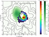Fig. C.1.

Median continuum in PSF-subtracted cube. The green coloured region corresponds to all islands of at least 5 contiguous spaxels with a mean continuum, measured over 3-4.2 μm, detected at the 1σ level. We compare it here to the contours of the initial non-PSF-subtracted quasar cube. We also indicate the location of the significant Hβ line emission envelope. The offset location of the continuum emission and its elliptical morphology indicate that it is likely not a PSF residual.

Appendix D: Spectra extracted from various emission regions in the NIRSpec IFU cube of J0313−1806

In Fig. D.1 we display spectra extracted within 0 $\overset{″}{.}$ $Mathematical equation: $ \overset{\prime \prime }{.} $$ 35 of regions A, B, and C defined in Section 4.1.

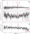Fig. D.1.

Spectra extracted from the PSF-subtracted NIRSpec IFU cube within circular apertures of radii 0 $\overset{″}{.}$ $Mathematical equation: $ \overset{\prime \prime }{.} $$ 35 at the regions A, B, and C (defined in Section 4.1). Region A corresponds to the Hβ nebula discussed in this paper. Region B corresponds to the extended continuum emission around the north-east of the quasar. Region C corresponds to a foreground galaxy at z = 2.3.

All Tables

Table 1.

Results of spectral fitting for J0313–1806.

In the text

All Figures

	Fig. A.2. Top: Three-spaxel aperture spectrum comparison for the datacube corrected with `WICKED` (blue) vs. uncorrected (yellow). Bottom: Percentage difference (grey) between the uncorrected and `WICKED` data.
In the text

Current usage metrics show cumulative count of Article Views (full-text article views including HTML views, PDF and ePub downloads, according to the available data) and Abstracts Views on Vision4Press platform.

Data correspond to usage on the plateform after 2015. The current usage metrics is available 48-96 hours after online publication and is updated daily on week days.

Initial download of the metrics may take a while.

[R1] Abramowicz, M. A. 2005, in Growing Black Holes: Accretion in a Cosmological Context, eds. A. Merloni, S. Nayakshin, & R. A. Sunyaev, 257 [Google Scholar]

[R2] Abramowicz, M. A., Czerny, B., Lasota, J. P., & Szuszkiewicz, E. 1988, ApJ, 332, 646 [Google Scholar]

[R3] Allen, R. J., Kacprzak, G. G., Glazebrook, K., et al. 2017, ApJ, 834, L11 [NASA ADS] [CrossRef] [Google Scholar]

[R4] Assef, R. J., Eisenhardt, P. R. M., Stern, D., et al. 2015, ApJ, 804, 27 [Google Scholar]

[R5] Astropy Collaboration (Robitaille, T. P., et al.) 2013, A&A, 558, A33 [NASA ADS] [CrossRef] [EDP Sciences] [Google Scholar]

[R6] Astropy Collaboration (Price-Whelan, A. M., et al.) 2018, AJ, 156, 123 [Google Scholar]

[R7] Astropy Collaboration (Price-Whelan, A. M., et al.) 2022, ApJ, 935, 167 [NASA ADS] [CrossRef] [Google Scholar]

[R8] Baldwin, J. A. 1977, ApJ, 214, 679 [NASA ADS] [CrossRef] [Google Scholar]

[R9] Baldwin, J. A., Phillips, M. M., & Terlevich, R. 1981, PASP, 93, 5 [Google Scholar]

[R10] Bañados, E., Venemans, B. P., Decarli, R., et al. 2016, ApJS, 227, 11 [Google Scholar]

[R11] Bañados, E., Venemans, B. P., Mazzucchelli, C., et al. 2018, Nature, 553, 473 [Google Scholar]

[R12] Bañados, E., Schindler, J.-T., Venemans, B. P., et al. 2023, ApJS, 265, 29 [CrossRef] [Google Scholar]

[R13] Bañados, E., Le Brun, V., Belladitta, S., et al. 2025a, MNRAS, 542, 1088 [Google Scholar]

[R14] Bañados, E., Momjian, E., Connor, T., et al. 2025b, Nat. Astron., 9, 293 [Google Scholar]

[R15] Baskin, A., & Laor, A. 2005, MNRAS, 358, 1043 [Google Scholar]

[R16] Baskin, A., & Laor, A. 2021, MNRAS, 508, 680 [NASA ADS] [CrossRef] [Google Scholar]

[R17] Baskin, A., Laor, A., & Stern, J. 2014a, MNRAS, 438, 604 [NASA ADS] [CrossRef] [Google Scholar]

[R18] Baskin, A., Laor, A., & Stern, J. 2014b, MNRAS, 445, 3025 [Google Scholar]

[R19] Belladitta, S., Moretti, A., Caccianiga, A., et al. 2020, A&A, 635, L7 [EDP Sciences] [Google Scholar]

[R20] Belladitta, S., Bañados, E., Xie, Z.-L., et al. 2025, A&A, 699, A335 [NASA ADS] [CrossRef] [EDP Sciences] [Google Scholar]

[R21] Bennert, N., Falcke, H., Schulz, H., Wilson, A. S., & Wills, B. J. 2002, ApJ, 574, L105 [NASA ADS] [CrossRef] [Google Scholar]

[R22] Bennert, N., Jungwiert, B., Komossa, S., Haas, M., & Chini, R. 2006, A&A, 459, 55 [NASA ADS] [CrossRef] [EDP Sciences] [Google Scholar]

[R23] Böker, T., Arribas, S., Lützgendorf, N., et al. 2022, A&A, 661, A82 [NASA ADS] [CrossRef] [EDP Sciences] [Google Scholar]

[R24] Boroson, T. A., & Green, R. F. 1992, ApJS, 80, 109 [Google Scholar]

[R25] Buchner, J., Georgakakis, A., Nandra, K., et al. 2015, ApJ, 802, 89 [Google Scholar]

[R26] Castor, J. I., Abbott, D. C., & Klein, R. I. 1975, ApJ, 195, 157 [Google Scholar]

[R27] Chen, Y., Luo, B., Brandt, W. N., et al. 2024, ApJ, 972, 191 [Google Scholar]

[R28] Circosta, C., Vignali, C., Gilli, R., et al. 2019, A&A, 623, A172 [NASA ADS] [CrossRef] [EDP Sciences] [Google Scholar]

[R29] Costa, T., Sijacki, D., & Haehnelt, M. G. 2015, MNRAS, 448, L30 [NASA ADS] [CrossRef] [Google Scholar]

[R30] D’Amato, Q., Gilli, R., Vignali, C., et al. 2020, A&A, 636, A37 [NASA ADS] [CrossRef] [EDP Sciences] [Google Scholar]

[R31] Davies, F. B., Hennawi, J. F., & Eilers, A.-C. 2019, ApJ, 884, L19 [Google Scholar]

[R32] de Graaff, A., Rix, H.-W., Naidu, R. P., et al. 2025, A&A, 701, A168 [NASA ADS] [CrossRef] [EDP Sciences] [Google Scholar]

[R33] Decarli, R., Loiacono, F., Farina, E. P., et al. 2024, A&A, 689, A219 [NASA ADS] [CrossRef] [EDP Sciences] [Google Scholar]

[R34] Diamond-Stanic, A. M., Fan, X., Brandt, W. N., et al. 2009, ApJ, 699, 782 [NASA ADS] [CrossRef] [Google Scholar]

[R35] Ding, X., Silverman, J. D., & Onoue, M. 2022, ApJ, 939, L28 [NASA ADS] [CrossRef] [Google Scholar]

[R36] Ding, X., Onoue, M., Silverman, J. D., et al. 2023, Nature, 621, 51 [NASA ADS] [CrossRef] [Google Scholar]

[R37] Draine, B. T. 2011, ApJ, 732, 100 [NASA ADS] [CrossRef] [Google Scholar]

[R38] Dultzin, D., Marziani, P., de Diego, J. A., et al. 2020, Front. Astron. Space Sci., 6, 80 [NASA ADS] [CrossRef] [Google Scholar]

[R39] Dumont, A., Neumayer, N., Seth, A. C., et al. 2025, A&A, 703, A54 [NASA ADS] [CrossRef] [EDP Sciences] [Google Scholar]

[R40] Ďurovčíková, D., Eilers, A.-C., Ishikawa, Y., et al. 2025, arXiv e-prints [arXiv:2510.09753] [Google Scholar]

[R41] Eilers, A.-C., Simcoe, R. A., Yue, M., et al. 2023, ApJ, 950, 68 [CrossRef] [Google Scholar]

[R42] Eldridge, J. J., Stanway, E. R., Xiao, L., et al. 2017, PASA, 34, e058 [Google Scholar]

[R43] Fan, X., Strauss, M. A., Gunn, J. E., et al. 1999, ApJ, 526, L57 [NASA ADS] [CrossRef] [Google Scholar]

[R44] Fan, X., Narayanan, V. K., Lupton, R. H., et al. 2001, AJ, 122, 2833 [Google Scholar]

[R45] Fan, X., Bañados, E., & Simcoe, R. A. 2023, ARA&A, 61, 373 [NASA ADS] [CrossRef] [Google Scholar]

[R46] Farina, E. P., Schindler, J.-T., Walter, F., et al. 2022, ApJ, 941, 106 [NASA ADS] [CrossRef] [Google Scholar]

[R47] Ferland, G. J., Porter, R. L., van Hoof, P. A. M., et al. 2013, Rev. Mex. Astron. Astrofis., 49, 137 [Google Scholar]

[R48] Ferrarese, L., & Merritt, D. 2000, ApJ, 539, L9 [Google Scholar]

[R49] Foroosh, H., Zerubia, J., & Berthod, M. 2002, IEEE Trans. Image Process., 11, 188 [Google Scholar]

[R50] Gardner, J. P., Mather, J. C., Clampin, M., et al. 2006, Space Sci. Rev., 123, 485 [Google Scholar]

[R51] Gebhardt, K., Kormendy, J., Ho, L. C., et al. 2000, ApJ, 543, L5 [CrossRef] [Google Scholar]

[R52] Gilli, R., Norman, C., Vignali, C., et al. 2014, A&A, 562, A67 [NASA ADS] [CrossRef] [EDP Sciences] [Google Scholar]

[R53] Gilli, R., Norman, C., Calura, F., et al. 2022, A&A, 666, A17 [NASA ADS] [CrossRef] [EDP Sciences] [Google Scholar]

[R54] Glikman, E., Lacy, M., LaMassa, S., et al. 2018, ApJ, 861, 37 [NASA ADS] [CrossRef] [Google Scholar]

[R55] Gloudemans, A. J., Duncan, K. J., Saxena, A., et al. 2022, A&A, 668, A27 [NASA ADS] [CrossRef] [EDP Sciences] [Google Scholar]

[R56] Goodrich, R. W. 1989, ApJ, 342, 224 [Google Scholar]

[R57] Greene, J. E., & Ho, L. C. 2005, ApJ, 630, 122 [NASA ADS] [CrossRef] [Google Scholar]

[R58] Greene, J. E., Zakamska, N. L., Ho, L. C., & Barth, A. J. 2011, ApJ, 732, 9 [NASA ADS] [CrossRef] [Google Scholar]

[R59] Gunasekera, C. M., van Hoof, P. A. M., Chatzikos, M., & Ferland, G. J. 2023, Res. Notes Am. Astron. Soc., 7, 246 [Google Scholar]

[R60] Guo, H., Shen, Y., & Wang, S. 2018, Astrophysics Source Code Library [record ascl:1809.008] [Google Scholar]

[R61] Ha, T., Dix, C., Matthews, B. M., et al. 2023, ApJ, 950, 97 [Google Scholar]

[R62] Habouzit, M., Li, Y., Somerville, R. S., et al. 2021, MNRAS, 503, 1940 [NASA ADS] [CrossRef] [Google Scholar]

[R63] Hainline, K. N., Hickox, R. C., Greene, J. E., et al. 2014, ApJ, 787, 65 [Google Scholar]

[R64] Häring, N., & Rix, H.-W. 2004, ApJ, 604, L89 [Google Scholar]

[R65] Hewett, P. C., Warren, S. J., Leggett, S. K., & Hodgkin, S. T. 2006, MNRAS, 367, 454 [Google Scholar]

[R66] Hopkins, P. F., Hernquist, L., Cox, T. J., et al. 2006, ApJS, 163, 1 [Google Scholar]

[R67] Huško, F., Lacey, C. G., Roper, W. J., et al. 2025, MNRAS, 537, 2559 [Google Scholar]

[R68] Ighina, L., Caccianiga, A., Moretti, A., et al. 2024, A&A, 692, A241 [NASA ADS] [CrossRef] [EDP Sciences] [Google Scholar]

[R69] Inayoshi, K., & Maiolino, R. 2025, ApJ, 980, L27 [Google Scholar]

[R70] Inayoshi, K., Visbal, E., & Haiman, Z. 2020, ARA&A, 58, 27 [NASA ADS] [CrossRef] [Google Scholar]

[R71] Ishibashi, W., Fabian, A. C., Ricci, C., & Celotti, A. 2018, MNRAS, 479, 3335 [CrossRef] [Google Scholar]

[R72] Ishibashi, W., Fabian, A. C., & Arakawa, N. 2021, MNRAS, 502, 3638 [NASA ADS] [CrossRef] [Google Scholar]

[R73] Ishikawa, Y., Zakamska, N. L., Shen, Y., et al. 2025, ApJ, 982, 22 [Google Scholar]

[R74] Iwasawa, K., Comastri, A., Vignali, C., et al. 2020, A&A, 639, A51 [NASA ADS] [CrossRef] [EDP Sciences] [Google Scholar]

[R75] Jahnke, K. 2025, Open J. Astrophys., 8, 9 [Google Scholar]

[R76] Jiang, L., McGreer, I. D., Fan, X., et al. 2016, ApJ, 833, 222 [Google Scholar]

[R77] Joh, K., Nagao, T., Wada, K., Terao, K., & Yamashita, T. 2021, PASJ, 73, 1152 [NASA ADS] [CrossRef] [Google Scholar]

[R78] Just, D. W., Brandt, W. N., Shemmer, O., et al. 2007, ApJ, 665, 1004 [Google Scholar]

[R79] Kakkad, D., Groves, B., Dopita, M., et al. 2018, A&A, 618, A6 [NASA ADS] [CrossRef] [EDP Sciences] [Google Scholar]

[R80] Kaspi, S., Smith, P. S., Netzer, H., et al. 2000, ApJ, 533, 631 [Google Scholar]

[R81] Kauffmann, G., Heckman, T. M., Tremonti, C., et al. 2003, MNRAS, 346, 1055 [Google Scholar]

[R82] Kennicutt, R. C., Jr. 1998, ARA&A, 36, 189 [Google Scholar]

[R83] Kewley, L. J., Groves, B., Kauffmann, G., & Heckman, T. 2006, MNRAS, 372, 961 [Google Scholar]

[R84] Kido, D., Ioka, K., Hotokezaka, K., Inayoshi, K., & Irwin, C. M. 2025, MNRAS, 544, 3407 [Google Scholar]

[R85] Kormendy, J., & Ho, L. C. 2013, ARA&A, 51, 511 [Google Scholar]

[R86] Lambrides, E. L., Chiaberge, M., Heckman, T., et al. 2020, ApJ, 897, 160 [Google Scholar]

[R87] Lansbury, G. B., Banerji, M., Fabian, A. C., & Temple, M. J. 2020, MNRAS, 495, 2652 [Google Scholar]

[R88] Lanzuisi, G., Delvecchio, I., Berta, S., et al. 2017, A&A, 602, A123 [NASA ADS] [CrossRef] [EDP Sciences] [Google Scholar]

[R89] Law, D. R., Morrison, J. E., Argyriou, I., et al. 2023, AJ, 166, 45 [NASA ADS] [CrossRef] [Google Scholar]

[R90] Leighly, K. M., Halpern, J. P., Jenkins, E. B., & Casebeer, D. 2007, ApJS, 173, 1 [NASA ADS] [CrossRef] [Google Scholar]

[R91] Li, Q., Narayanan, D., & Davé, R. 2019, MNRAS, 490, 1425 [CrossRef] [Google Scholar]

[R92] Liu, G., Zakamska, N. L., & Greene, J. E. 2014, MNRAS, 442, 1303 [NASA ADS] [CrossRef] [Google Scholar]

[R93] Liu, T., Tozzi, P., Wang, J.-X., et al. 2017, ApJS, 232, 8 [NASA ADS] [CrossRef] [Google Scholar]

[R94] Liu, W., Fan, X., Yang, J., et al. 2024, ApJ, 976, 33 [Google Scholar]

[R95] Lodieu, N., Pinfield, D. J., Leggett, S. K., et al. 2007, MNRAS, 379, 1423 [NASA ADS] [CrossRef] [Google Scholar]

[R96] Loiacono, F., Decarli, R., Mignoli, M., et al. 2024, A&A, 685, A121 [NASA ADS] [CrossRef] [EDP Sciences] [Google Scholar]

[R97] Luo, B., Brandt, W. N., Hall, P. B., et al. 2015, ApJ, 805, 122 [Google Scholar]

[R98] Lupi, A., Quadri, G., Volonteri, M., Colpi, M., & Regan, J. A. 2024a, A&A, 686, A256 [NASA ADS] [CrossRef] [EDP Sciences] [Google Scholar]

[R99] Lupi, A., Trinca, A., Volonteri, M., Dotti, M., & Mazzucchelli, C. 2024b, A&A, 689, A128 [NASA ADS] [CrossRef] [EDP Sciences] [Google Scholar]

[R100] Luridiana, V., Morisset, C., & Shaw, R. A. 2015, A&A, 573, A42 [NASA ADS] [CrossRef] [EDP Sciences] [Google Scholar]

[R101] Lusso, E., Comastri, A., Vignali, C., et al. 2010, A&A, 512, A34 [NASA ADS] [CrossRef] [EDP Sciences] [Google Scholar]

[R102] Lyke, B. W., Higley, A. N., McLane, J. N., et al. 2020, ApJS, 250, 8 [NASA ADS] [CrossRef] [Google Scholar]

[R103] Madau, P., & Haardt, F. 2024, ApJ, 976, L24 [Google Scholar]

[R104] Magorrian, J., Tremaine, S., Richstone, D., et al. 1998, AJ, 115, 2285 [Google Scholar]

[R105] Maiolino, R., & Rieke, G. H. 1995, ApJ, 454, 95 [Google Scholar]

[R106] Marcotulli, L., Connor, T., Bañados, E., et al. 2025, ApJ, 979, L6 [Google Scholar]

[R107] Marshall, M. A., Perna, M., Willott, C. J., et al. 2023, A&A, 678, A191 [NASA ADS] [CrossRef] [EDP Sciences] [Google Scholar]

[R108] Marshall, M. A., Yue, M., Eilers, A.-C., et al. 2025, A&A, 702, A50 [NASA ADS] [CrossRef] [EDP Sciences] [Google Scholar]

[R109] Martínez-Aldama, M. L., del Olmo, A., Marziani, P., et al. 2018, A&A, 618, A179 [NASA ADS] [CrossRef] [EDP Sciences] [Google Scholar]

[R110] Marziani, P., Sulentic, J. W., Zwitter, T., Dultzin-Hacyan, D., & Calvani, M. 2001, ApJ, 558, 553 [NASA ADS] [CrossRef] [Google Scholar]

[R111] Marziani, P., Dultzin, D., Sulentic, J. W., et al. 2018, Front. Astron. Space Sci., 5, 6 [CrossRef] [Google Scholar]

[R112] Matsuoka, Y., Onoue, M., Kashikawa, N., et al. 2016, ApJ, 828, 26 [Google Scholar]

[R113] Matsuoka, Y., Iwasawa, K., Onoue, M., et al. 2018a, ApJS, 237, 5 [Google Scholar]

[R114] Matsuoka, Y., Onoue, M., Kashikawa, N., et al. 2018b, PASJ, 70, S35 [Google Scholar]

[R115] Matsuoka, Y., Iwasawa, K., Onoue, M., et al. 2019, ApJ, 883, 183 [Google Scholar]

[R116] Matsuoka, Y., Iwasawa, K., Onoue, M., et al. 2022, ApJS, 259, 18 [NASA ADS] [CrossRef] [Google Scholar]

[R117] Matsuoka, Y., Onoue, M., Iwasawa, K., et al. 2023, ApJ, 949, L42 [NASA ADS] [CrossRef] [Google Scholar]

[R118] Matsuoka, Y., Iwasawa, K., Onoue, M., et al. 2025, ApJS, 280, 68 [Google Scholar]

[R119] Mazzolari, G., Übler, H., Maiolino, R., et al. 2024, A&A, 691, A345 [NASA ADS] [CrossRef] [EDP Sciences] [Google Scholar]

[R120] Mazzucchelli, C., Bischetti, M., D’Odorico, V., et al. 2023, A&A, 676, A71 [NASA ADS] [CrossRef] [EDP Sciences] [Google Scholar]

[R121] Mechtley, M., Windhorst, R. A., Ryan, R. E., et al. 2012, ApJ, 756, L38 [NASA ADS] [CrossRef] [Google Scholar]

[R122] Miller, J. M. 2007, ARA&A, 45, 441 [NASA ADS] [CrossRef] [Google Scholar]

[R123] Morisset, C. 2013, Astrophysics Source Code Library [record ascl:1304.020] [Google Scholar]

[R124] Mortlock, D. J., Patel, M., Warren, S. J., et al. 2009, A&A, 505, 97 [NASA ADS] [CrossRef] [EDP Sciences] [Google Scholar]

[R125] Mortlock, D. J., Warren, S. J., Venemans, B. P., et al. 2011, Nature, 474, 616 [Google Scholar]

[R126] Murray, N., Chiang, J., Grossman, S. A., & Voit, G. M. 1995, ApJ, 451, 498 [NASA ADS] [CrossRef] [Google Scholar]

[R127] Nagao, T., Maiolino, R., & Marconi, A. 2006, A&A, 447, 863 [NASA ADS] [CrossRef] [EDP Sciences] [Google Scholar]

[R128] Naidu, R. P., Matthee, J., Katz, H., et al. 2025, arXiv e-prints [arXiv:2503.16596] [Google Scholar]

[R129] Nanni, R., Vignali, C., Gilli, R., Moretti, A., & Brandt, W. N. 2017, A&A, 603, A128 [NASA ADS] [CrossRef] [EDP Sciences] [Google Scholar]

[R130] Netzer, H. 2015, ARA&A, 53, 365 [Google Scholar]

[R131] Netzer, H., Shemmer, O., Maiolino, R., et al. 2004, ApJ, 614, 558 [NASA ADS] [CrossRef] [Google Scholar]

[R132] Ni, Q., Brandt, W. N., Luo, B., et al. 2018, MNRAS, 480, 5184 [NASA ADS] [Google Scholar]

[R133] Ni, Y., Di Matteo, T., Gilli, R., et al. 2020, MNRAS, 495, 2135 [NASA ADS] [CrossRef] [Google Scholar]

[R134] Ni, Q., Brandt, W. N., Luo, B., et al. 2022, MNRAS, 511, 5251 [NASA ADS] [CrossRef] [Google Scholar]

[R135] Nicholls, D. C., Sutherland, R. S., Dopita, M. A., Kewley, L. J., & Groves, B. A. 2017, MNRAS, 466, 4403 [Google Scholar]

[R136] Nikołajuk, M., & Walter, R. 2012, MNRAS, 420, 2518 [CrossRef] [Google Scholar]

[R137] Onoue, M., Kashikawa, N., Matsuoka, Y., et al. 2019, ApJ, 880, 77 [Google Scholar]

[R138] Osterbrock, D. E., & Ferland, G. J. 2006, Astrophysics of Gaseous Nebulae and Active Galactic Nuclei [Google Scholar]

[R139] Osterbrock, D. E., & Pogge, R. W. 1985, ApJ, 297, 166 [Google Scholar]

[R140] Park, D., Barth, A. J., Ho, L. C., & Laor, A. 2022, ApJS, 258, 38 [NASA ADS] [CrossRef] [Google Scholar]

[R141] Peca, A., Cappelluti, N., Urry, C. M., et al. 2023, ApJ, 943, 162 [NASA ADS] [CrossRef] [Google Scholar]

[R142] Perna, M., Arribas, S., Marshall, M., et al. 2023, A&A, 679, A89 [NASA ADS] [CrossRef] [EDP Sciences] [Google Scholar]

[R143] Peterson, B. 2006, in The Broad-Line Region in Active Galactic Nuclei, eds. D. Alloin, R. Johnson, & P. Lira (Berlin, Heidelberg: Springer), 77 [Google Scholar]

[R144] Plotkin, R. M., Shemmer, O., Trakhtenbrot, B., et al. 2015, ApJ, 805, 123 [Google Scholar]

[R145] Pu, X., Luo, B., Brandt, W. N., et al. 2020, ApJ, 900, 141 [Google Scholar]

[R146] Pudoka, M., Wang, F., Fan, X., et al. 2025, ApJ, 987, 198 [Google Scholar]

[R147] Quadri, G., Trinca, A., Lupi, A., Colpi, M., & Volonteri, M. 2025, A&A, 704, A248 [NASA ADS] [CrossRef] [EDP Sciences] [Google Scholar]

[R148] Reed, S. L., McMahon, R. G., Banerji, M., et al. 2015, MNRAS, 454, 3952 [Google Scholar]

[R149] Reines, A. E., & Volonteri, M. 2015, ApJ, 813, 82 [NASA ADS] [CrossRef] [Google Scholar]

[R150] Ren, W., Guo, H., Shen, Y., et al. 2024, ApJ, 974, 153 [NASA ADS] [CrossRef] [Google Scholar]

[R151] Richards, G. T., Lacy, M., Storrie-Lombardi, L. J., et al. 2006, ApJS, 166, 470 [Google Scholar]

[R152] Rieke, M. J., Kelly, D. M., Misselt, K., et al. 2023, PASP, 135, 028001 [CrossRef] [Google Scholar]

[R153] Rivera, A. B., Richards, G. T., Hewett, P. C., & Rankine, A. L. 2020, ApJ, 899, 96 [NASA ADS] [CrossRef] [Google Scholar]

[R154] Rivera, A. B., Richards, G. T., Gallagher, S. C., et al. 2022, ApJ, 931, 154 [Google Scholar]

[R155] Rupke, D. S. N. 2014, IFSFIT: Spectral Fitting for Integral Field Spectrographs [Google Scholar]

[R156] Rupke, D. S. N., & Veilleux, S. 2013, ApJ, 768, 75 [Google Scholar]

[R157] Rupke, D. S. N., Schweitzer, M., Viola, V., et al. 2021, QUESTFIT: Fitter for Mid-Infrared Galaxy Spectra [Google Scholar]

[R158] Rusakov, V., Watson, D., Nikopoulos, G. P., et al. 2025, arXiv e-prints [arXiv:2503.16595] [Google Scholar]

[R159] Schindler, J.-T., Bañados, E., Connor, T., et al. 2023, ApJ, 943, 67 [NASA ADS] [CrossRef] [Google Scholar]

[R160] Schmitt, H. R., Donley, J. L., Antonucci, R. R. J., et al. 2003, ApJ, 597, 768 [NASA ADS] [CrossRef] [Google Scholar]

[R161] Scholtz, J., Maiolino, R., D’Eugenio, F., et al. 2025, A&A, 697, A175 [NASA ADS] [CrossRef] [EDP Sciences] [Google Scholar]

[R162] Scoville, N., Lee, N., Vanden Bout, P., et al. 2017, ApJ, 837, 150 [Google Scholar]

[R163] Shemmer, O., Trakhtenbrot, B., Anderson, S. F., et al. 2010, ApJ, 722, L152 [NASA ADS] [CrossRef] [Google Scholar]

[R164] Shen, Y., & Ho, L. C. 2014, Nature, 513, 210 [NASA ADS] [CrossRef] [Google Scholar]

[R165] Shen, Y., Wu, J., Jiang, L., et al. 2019, ApJ, 873, 35 [Google Scholar]

[R166] Shen, Y., Grier, C. J., Horne, K., et al. 2024, ApJS, 272, 26 [NASA ADS] [CrossRef] [Google Scholar]

[R167] Stanway, E. R., & Eldridge, J. J. 2018, MNRAS, 479, 75 [NASA ADS] [CrossRef] [Google Scholar]

[R168] Steffen, A. T., Strateva, I., Brandt, W. N., et al. 2006, AJ, 131, 2826 [Google Scholar]

[R169] Stern, J., & Laor, A. 2013, MNRAS, 431, 836 [NASA ADS] [CrossRef] [Google Scholar]

[R170] Stern, J., Behar, E., Laor, A., Baskin, A., & Holczer, T. 2014a, MNRAS, 445, 3011 [NASA ADS] [CrossRef] [Google Scholar]

[R171] Stern, J., Laor, A., & Baskin, A. 2014b, MNRAS, 438, 901 [NASA ADS] [CrossRef] [Google Scholar]

[R172] Stern, J., Faucher-Giguère, C.-A., Zakamska, N. L., & Hennawi, J. F. 2016, ApJ, 819, 130 [CrossRef] [Google Scholar]

[R173] Stone, H., Orchard, M., Chang, E.-C., & Martucci, S. 2001, IEEE Trans. Geosci. Remote Sens., 39, 2235 [Google Scholar]

[R174] Stone, M. A., Lyu, J., Rieke, G. H., & Alberts, S. 2023, ApJ, 953, 180 [NASA ADS] [CrossRef] [Google Scholar]

[R175] Storey, P. J., & Zeippen, C. J. 2000, MNRAS, 312, 813 [NASA ADS] [CrossRef] [Google Scholar]

[R176] Sulentic, J. W., Zwitter, T., Marziani, P., & Dultzin-Hacyan, D. 2000, ApJ, 536, L5 [Google Scholar]

[R177] Tacconi, L. J., Genzel, R., Saintonge, A., et al. 2018, ApJ, 853, 179 [Google Scholar]

[R178] Temple, M. J., Banerji, M., Hewett, P. C., et al. 2019, MNRAS, 487, 2594 [Google Scholar]

[R179] Timlin, J. D., III., Brandt, W. N., Zhu, S., et al. 2020, MNRAS, 498, 4033 [NASA ADS] [CrossRef] [Google Scholar]

[R180] Trefoloni, B., Carniani, S., Bertola, E., et al. 2025, A&A, submitted [arXiv:2509.07064] [Google Scholar]

[R181] Übler, H., Maiolino, R., Pérez-González, P. G., et al. 2024, MNRAS, 531, 355 [CrossRef] [Google Scholar]

[R182] Urry, C. M., & Padovani, P. 1995, PASP, 107, 803 [NASA ADS] [CrossRef] [Google Scholar]

[R183] Vayner, A., Zakamska, N. L., Ishikawa, Y., et al. 2024, ApJ, 960, 126 [NASA ADS] [CrossRef] [Google Scholar]

[R184] Vayner, A., Díaz-Santos, T., Eisenhardt, P. R. M., et al. 2025, ApJ, 989, 230 [Google Scholar]

[R185] Veilleux, S., & Osterbrock, D. E. 1987, ApJS, 63, 295 [Google Scholar]

[R186] Veilleux, S., Liu, W., Vayner, A., et al. 2023, ApJ, 953, 56 [NASA ADS] [CrossRef] [Google Scholar]

[R187] Vestergaard, M., & Osmer, P. S. 2009, ApJ, 699, 800 [Google Scholar]

[R188] Vestergaard, M., & Peterson, B. M. 2006, ApJ, 641, 689 [Google Scholar]

[R189] Vietri, G., Piconcelli, E., Bischetti, M., et al. 2018, A&A, 617, A81 [NASA ADS] [CrossRef] [EDP Sciences] [Google Scholar]

[R190] Vito, F., Brandt, W. N., Yang, G., et al. 2018, MNRAS, 473, 2378 [Google Scholar]

[R191] Vito, F., Brandt, W. N., Bauer, F. E., et al. 2019a, A&A, 630, A118 [NASA ADS] [CrossRef] [EDP Sciences] [Google Scholar]

[R192] Vito, F., Brandt, W. N., Bauer, F. E., et al. 2019b, A&A, 628, L6 [NASA ADS] [CrossRef] [EDP Sciences] [Google Scholar]

[R193] Volonteri, M., & Begelman, M. C. 2010, MNRAS, 409, 1022 [Google Scholar]

[R194] Wang, J.-M., Qiu, J., Du, P., & Ho, L. C. 2014, ApJ, 797, 65 [NASA ADS] [CrossRef] [Google Scholar]

[R195] Wang, F., Fan, X., Yang, J., et al. 2017, ApJ, 839, 27 [Google Scholar]

[R196] Wang, F., Yang, J., Fan, X., et al. 2021, ApJ, 907, L1 [Google Scholar]

[R197] Wang, B., Ishikawa, Y., Hennawi, J. F., et al. 2025, MNRAS, 544, 687 [Google Scholar]

[R198] Wolf, J., Salvato, M., Coffey, D., et al. 2020, MNRAS, 492, 3580 [NASA ADS] [CrossRef] [Google Scholar]

[R199] Wolf, J., Salvato, M., Belladitta, S., et al. 2024, A&A, 691, A30 [NASA ADS] [CrossRef] [EDP Sciences] [Google Scholar]

[R200] Wu, Q., & Shen, Y. 2022, ApJS, 263, 42 [NASA ADS] [CrossRef] [Google Scholar]

[R201] Wu, J., Brandt, W. N., Hall, P. B., et al. 2011, ApJ, 736, 28 [NASA ADS] [CrossRef] [Google Scholar]

[R202] Wu, X.-B., Wang, F., Fan, X., et al. 2015, Nature, 518, 512 [Google Scholar]

[R203] Wylezalek, D., Vayner, A., Rupke, D. S. N., et al. 2022, ApJ, 940, L7 [NASA ADS] [CrossRef] [Google Scholar]

[R204] Yang, J., Wang, F., Fan, X., et al. 2020, ApJ, 897, L14 [Google Scholar]

[R205] Yang, J., Wang, F., Fan, X., et al. 2021, ApJ, 923, 262 [NASA ADS] [CrossRef] [Google Scholar]

[R206] Yi, W., Vivek, M., Brandt, W. N., et al. 2019, ApJ, 870, L25 [Google Scholar]

[R207] York, D. G., Adelman, J., Anderson, J. E., Jr., et al. 2000, AJ, 120, 1579 [NASA ADS] [CrossRef] [Google Scholar]

[R208] Yue, M., Eilers, A.-C., Simcoe, R. A., et al. 2024, ApJ, 966, 176 [NASA ADS] [CrossRef] [Google Scholar]

[R209] Zakamska, N. L., Hamann, F., Pâris, I., et al. 2016, MNRAS, 459, 3144 [NASA ADS] [CrossRef] [Google Scholar]

[R210] Zhang, K., Wang, T.-G., Gaskell, C. M., & Dong, X.-B. 2013, ApJ, 762, 51 [Google Scholar]

Shedding the envelope: JWST reveals a kiloparsec-scale [O III]-weak Balmer shell around a z = 7.64 quasar

1. Introduction

2. Observations and data reduction

2.1. JWST/NIRSpec IFU pointings

2.2. Data reduction

3. Physical properties of the black hole

3.1. Spectral fitting

3.2. Black hole mass and Eddington rate

4. Extended nebular emission

4.1. Point spread function modeling

4.2. Balmer kinematic moment maps

5. Discussion

5.1. Suppressed nuclear [O III] emission

5.1.1. A possible high-z weak line quasar

5.1.2. J0313–1806 and the quasar main sequence

5.2. Suppressed extended [O III] emission

5.2.1. Photoionization simulations

5.2.2. Hβ shell energetics

5.3. Obscured black hole growth and fossil evidence for blowout phase

6. Conclusions

Acknowledgments

References

Appendix A: Post-processing PSF undersampling with WICKED

Appendix B: Determination of quasar spectrum extraction radius

Appendix C: Tentative detection of extended continuum emission

Appendix D: Spectra extracted from various emission regions in the NIRSpec IFU cube of J0313−1806

All Tables

All Figures

Shedding the envelope: JWST reveals a kiloparsec-scale [O III]-weak Balmer shell around a z = 7.64 quasar

5.1. Suppressed nuclear [O III] emission

5.2. Suppressed extended [O III] emission