| Issue |
A&A
Volume 698, June 2025
|
|
|---|---|---|
| Article Number | A228 | |
| Number of page(s) | 9 | |
| Section | Astrophysical processes | |
| DOI | https://doi.org/10.1051/0004-6361/202452141 | |
| Published online | 17 June 2025 | |
Long-term stability estimation of ensemble pulsar timescales with NICER observations
1
School of Aerospace Science and Technology, Xidian University, Xi’an, China
2
Shaanxi Key Laboratory of Space Extreme Detection, Xi’an, China
3
Peng Cheng Laboratory, Shenzhen, China
4
Academy of Advanced Interdisciplinary Research, Xidian University, Xi’an, China
5
National Time Service Center (NTSC), Chinese Academy of Sciences (CAS), Xi’an, China
6
Xi’an Institute of Surveying and Mapping, Xi’an 710054, China
⋆ Corresponding author: This email address is being protected from spambots. You need JavaScript enabled to view it.
Received:
6
September
2024
Accepted:
21
April
2025
Abstract
Context. The ensemble pulsar timescale (EPT), derived from the rotation rates of millisecond pulsars, exhibits a stability comparable to the International Atomic Time (TAI) over a decade.
Aims. This research aims to establish an X-ray-based EPT and evaluate its stability through a comprehensive analysis of 7.3 years of NICER observations of PSR B1937+21 (PSR J1939+2134) and PSR B1821-24 (PSR J1824-2452A).
Methods. By leveraging an advanced parameter fitting technique, we refined the timing parameters, and achieved notable convergence in timing residuals. To reduce the impact of prominent white noise characteristics inherent in X-ray data, we devised an integrated timing residuals generation framework. This framework incorporates the subtraction of red noise, using both Gaussian process regression (GPR) and Bayesian factor analysis methodologies. Additionally, we introduced an enhanced Wiener filtering algorithm, tailored specifically to enhance the stability of the EPT, which further refined our analysis and ensured robust results.
Results. The root mean square errors (RMSE) of the timing residuals were determined to be 4.17 μs for PSR B1937+21 and 25.07 μs for PSR B1821-24. We find strong evidence of red noise in the 7.3-year data of both pulsars and, combined with our proposed simulation residual generation framework, successfully construct an ensemble pulsar timescale. The 7.3-year EPT stability was improved to 4.19 × 10⁻¹⁵, which represents an improvement of one order of magnitude compared to conventional methods.
Conclusions. The EPT framework developed herein facilitates reproducible experiments, and yields statistically robust stability metrics derived from X-ray data. Notably, the tailored Wiener filtering algorithm, which is designed to address the unique challenges of X-ray data, significantly increases the stability of the EPT.
Key words: methods: data analysis / methods: observational / pulsars: general
© The Authors 2025
 Open Access article, published by EDP Sciences, under the terms of the Creative Commons Attribution License (https://creativecommons.org/licenses/by/4.0), which permits unrestricted use, distribution, and reproduction in any medium, provided the original work is properly cited.
This article is published in open access under the Subscribe to Open model. This email address is being protected from spambots. You need JavaScript enabled to view it. to support open access publication.
1. Introduction
International Atomic Time (TAI) is a timescale established and maintained by the Bureau International des Poids et Mesures (BIPM) using about 460 atomic clocks and several frequency standards from about 89 timing laboratories worldwide. TAI represents an ensemble timescale that is susceptible to accumulated errors capable of influencing its long-term stability. Pulsars emit steady periodic pulse signals outward, thereby establishing a timescale known as pulsar time (Petit 1996; Taylor 1991). They demonstrate remarkable long-term stability, with the highest stability surpassing 10−16 (Allan 1987), which renders them ideal for monitoring the enduring stability of TAI (Hartnett & Luiten 2010; Li et al. 2020). The stability of pulsar timing refers to the degree of random fluctuations in the rotation frequency of pulsars influenced by various sources of noise. It indicates the deviation of a pulsar’s rotation frequency or phase relative to the average frequency or phase over a specified time period, which serves as a crucial metric for assessing pulsar timing performance. Furthermore, pulsar timing can be employed to improve the solar system planetary ephemeris by detecting perturbations of the Earth (Foster & Backer 1990), while also offering essential evidence for the detection of gravitational waves (Weisberg & Taylor 1981; Jenet et al. 2005).
After recording the pulse times of arrival (TOAs) from a specific pulsar at a radio observatory, these pulse TOAs should be calibrated to accurately reflect the arrival times in an inertial reference frame (Edwards et al. 2006). Once the impact of both intrinsic and extrinsic noise sources are mitigated (including effects arising from the relative motion between the pulsar and observatory, instrumental errors, and signal propagation delays), the pulse TOAs can be regarded as an equivalent comparison between the pulsar’s clock and a reference atomic clock. Generally, public research on pulsar timing mainly relies on radio observations. In 2010, the International Pulsar Timing Array (IPTA) was formally established (Hobbs et al. 2010). The primary objective of IPTA is to detect and characterize low-frequency gravitational waves by timing approximately 100 millisecond pulsars (MSPs) globally and to establish a pulsar-based reference timescale. The current formal members of this organization include the Australian Parkes Pulsar Timing Array (PPTA) (Reardon et al. 2021), the North American Nanohertz Observatory for Gravitational Waves (NANOGrav) (Alam et al. 2020), the European Pulsar Timing Array (EPTA) (Desvignes et al. 2016; EPTA Collaboration 2023; Chen et al. 2021), and the Indian Pulsar Timing Array (InPTA) (Paul et al. 2019; Tarafdar et al. 2022; Srivastava et al. 2023). Observing members consist of the MeerKAT Pulsar Timing Array (MPTA) in South Africa (Johnston et al. 2020; Miles et al. 2022; Spiewak et al. 2022) and the Chinese Pulsar Timing Array (CPTA) (Lee et al. 2012; Xu et al. 2023). The IPTA team has conducted long-term observations of over 60 MSPs (Manchester 2013), with some accumulating more than 20 years of data. The ensemble pulsar timescal (EPT) constructed using IPTA’s DR1 (Verbiest et al. 2016) or DR2 (Perera et al. 2019) data demonstrates long-term stability comparable to or slightly better than atomic time (Zharov et al. 2019; Rodin & Fedorova 2018). After removing linear and quadratic terms, it exhibits trends similar to TT (BIPM), which accurately reveals high-order systematic errors in TAI (Hobbs et al. 2012, 2020), and thereby demonstrates the viability of pulsar timing for monitoring atomic time (Zhao et al. 2023). Given that the precision of pulsar timing is largely dependent on the receiving antenna area, the completion of Five-hundred-meter Aperture Spherical radio Telescope (FAST) in recent years has provided an excellent opportunity for establishing high-precision ensemble pulsar timescale (EPT) (Zhou et al. 2021) simulated and evaluated ten-year timing datasets for several MSPs based on FAST observations, and achieved a stability of 1.39 × 10⁻¹⁶.
In contrast to radio observations, X-ray observations conducted in outer space avoid atmospheric dispersion effects, thereby enhancing the precision of pulse TOA measurements and making X-ray data more suitable for constructing comprehensive pulsar timing. Due to the extremely faint signals emitted by most MSPs in the X-ray band and the inherent limitations of X-ray observations, such as the difficulty in increasing the detector area, several pulsars known for their exceptional stability in the radio band (e.g., J0437-4715) exhibit significantly reduced signal-to-noise ratios (S/N) in the X-ray band. Additionally, many MSPs display thermal X-ray pulsations with considerably broader peaks compared to those observed in the radio band (Deneva et al. 2019; Bogdanov 2017), which further impacts the precision of pulse TOA measurements. However, two notable exceptions, PSR B1937+21 and PSR B1821-24, exhibit remarkably narrow nonthermal X-ray pulsations, making them highly suitable candidates for EPT (Kawai et al. 1998). These two pulsars have undergone extensive long-term observations by several prominent radio telescopes, which has led to significant successes in evaluating their stability (Backer et al. 1982; Kaspi et al. 1994; Lyne 1987; Cognard et al. 1996; Hazboun et al. 2022). Nonetheless, elevating their stability and constructing EPT in the X-ray spectrum still remain challenging due to weak X-ray emissions and limited detector areas. The situation has seen significant improvement with the emergence of the Neutron Star Interior Composition Explorer (NICER), due to its robust X-ray observation capabilities and a remarkable time resolution of less than 100 ns (Gendreau et al. 2016; Prigozhin et al. 2016; Gendreau & Arzoumanian 2017). Deneva et al. 2019 assessed the one-year stabilities of PSR B1937+21 and PSR B1821-24 using NICER observations, and obtained stabilities of 3.1 × 10⁻¹⁴ and 1.5 × 10⁻¹², respectively. However, longer-term stability investigations have not been conducted due to the limited duration of the data. Sun et al. 2023 determined that the five-year NICER stability of PSR B1937+21 is 1.7 × 10⁻¹⁴, which demonstrates that the pulsar’s rotation exhibits exceptional stability over an extended observation period.
To address the current gap in the research on constructing EPT for X-ray data, this paper introduces a comprehensive X-ray pulsar timing processing framework and establishes EPT over a 7.3-year period for PSR B1937+21 and PSR B1821-24. The key contributions of this study can be summarized as follows. Firstly, this study processed and obtained the 7.3 years NICER timing residuals for the two pulsars, PSR B1937+21 and PSR B1821-24. Secondly, an X-ray pulsar timing processing framework was introduced, which includes a comprehensive noise analysis component that detected significant evidence of red noise present in both pulsars using Bayesian factors, and employed noise model fitting to better model ensemble timing residuals, demonstrating a substantial improvement over the classical cubic spline interpolation method. Lastly, an enhanced Wiener filtering algorithm was proposed for constructing ensemble pulsar timing, specifically designed to mitigate the high white noise levels inherent in X-ray observations.
The remainder of this paper is structured as follows. Section 2 details the processing procedures for NICER data. Section 3 describes the framework and algorithms developed for X-ray pulsar timing. Section 4 presents an analysis of the experimental results. Finally, Section 5 provides the conclusions and discussion.
2. Observations and data processing
Most MSPs typically exhibit low flux in the X-ray band, which results in a low signal-to-noise ratio of the pulse profile and subsequently affects the accuracy of pulse TOAs. Thus, the implementation of certain preprocessing techniques becomes essential to augment the S/N of pulsar profiles, which include the screenings of the energy and flux rate ranges, and S/N (Sun et al. 2023). In terms of optimal energy range screening, we employed a step size of 0.05 keV and calculated the chi-square values of pulsar profiles across various energy segments. The optimal energy ranges determined for the two pulsars are 1.1–6.55 keV for PSR B1937+21 and 0.8–5.5 keV for PSR B1821-24. For optimal flux rate range screening, we employed an eight-second observation interval with a flux rate threshold of 2 cnts/s. Segments with a photon flux rate that surpasses this threshold were excluded, since it indicates prevalent noise. Additionally, we excluded individual observations with notably low S/Ns or inadequate photon counts. The data preprocessing results for PSR B1937+21 and PSR B1821-24 are presented in Table 1.
NICER observations of PSR B1937+21 and PSR B1821-24.
We performed time corrections using the “barycorr” command within the HEASoft software. The Einstein delay was modeled using 127 sine periodic terms, with a precision of up to 100 ns (Fairhead & Bretagnon 1990). Due to the relatively lower precision of pulse TOAs in X-ray timing data, an enhanced parameter fitting framework was adopted to iteratively refine timing parameters by incorporating TOAs across the entire observation span (Sun et al. 2023). The timing residuals for the two pulsars, obtained by fitting the timing parameters, are illustrated in Figure 1. The residuals for PSR B1937+21 show a smaller amplitude of red noise, with a root mean square (RMS) of 4.17 μs, while PSR B1821-24 exhibits significant fluctuations and strong red noise, with a RMS of 25.07 μs. The fitted timing parameters are detailed in Table 2.
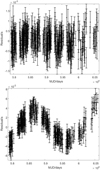 |
Fig. 1. Timing residuals after fitting the timing model: (a) PSR B1937+21, (b) PSR B1821-24. |
Timing parameters for PSR B1937+21 and PSR B1821-24.
To compare the stability between NICER and radio data, we analyzed NANOGrav data for PSR B1937+21 and PPTA data for PSR B1821-24, as depicted in Figure 2. For PSR B1937+21, the timing residuals in the radio data are generally within ±5 μs, although certain data points exhibit larger error bars exceeding 15 μs. The timing residuals for PSR B1821-24 fall within the range of ±30 μs. In the radio timing residuals of PSR B1821-24, previous studies have demonstrated the presence of discernible red noise (Vivekanand 2019; The NANOGrav Collaboration 2019).
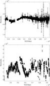 |
Fig. 2. Radio timing residuals for PSR B1937+21 and PSR B1821-24. (a) PSR B1937+21, (b) PSR B1821-24. |
3. Ensemble pulsar timing analysis
Pulsar timing residuals are affected by various sources of stochastic noise, with many of these noise components being independent from each other. To mitigate the influence of independent noise in timing data, the ensemble averaging technique can be implemented, for which the most classic algorithm is the weighted average method (Kaspi 1995; Petit et al. 1993). By conducting this method, the constructed EPT achieved a stability of 2 × 10⁻¹⁴ over a period of 2.5 years, outperforming the stability calculated from individual pulsars (Petit 1996). Afterward, wavelet filtering and Wiener filtering algorithms were successively applied to EPT. Following the evaluation of seven-year data from the Arecibo Observatory for PSR B1855+09 and PSR B1937+21, the Wiener filtering algorithm exhibits excellent performance, achieving a stability of 1.7 × 10⁻¹⁵ (Zhong & Yang 2007). Furthermore, a joint algorithm combining wavelet decomposition with Wiener filtering was proposed and achieved a level of stability surpassing that of other algorithms (Zhong & Yang 2007). In addition, a bispectral filtering algorithm was introduced for constructing ensemble pulsar timing. The results show that the bispectral filtering algorithm can effectively reduce the influence of observation noise and improve the stability of ensemble pulsar time compared to the classic weighting method (Zhou et al. 2021). By utilizing 8.2-year data obtained from the above two pulsars, Rodin improved the stability to (0.8 ± 1.9) × 10−15 (Rodin 2008).
3.1. Ensemble pulsar timing framework
In the construction of ensemble pulsar timing, it is essential to have simultaneous observational data from different pulsars. Radio observations typically employ cubic spline interpolation to connect these data points. Given the high precision of radio TOAs, this method introduces minimal error. However, X-ray observations, which are subject to significant white noise and large gaps between observations, present a challenge. In such cases, cubic spline interpolation can result in substantial errors due to the large gaps between the data points. Moreover, this method generates only one set of deterministic timing residuals for stability analysis, which renders it insufficient for accurately representing the pulsar’s stability. To address this, we developed a framework for generating simulated residuals that incorporates red noise estimation, as illustrated in Figure 3. The framework consists of modeling both red noise and white noise, as well as extracting residual trends (such as clock offsets and gravitational wave signals). After removing the red noise, we rely on the randomness of the white noise and fixed trend components to generate simulated residuals, and we conduct multiple Monte Carlo experiments to achieve more accurate statistical results.
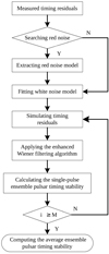 |
Fig. 3. Framework for generating ensemble pulsar timing residuals. |
The framework consists of two main components: noise modeling and residual simulation. Understanding timing noise is crucial for studying pulsars and advancing pulsar timing applications (Arzoumanian et al. 2018). The first step is to determine the presence of red noise in timing residuals by calculating the Bayesian factor. White noise has a uniform power spectral density, whereas red noise is concentrated at lower frequencies. To accurately identify variations related to the reference clock, it is essential to extract and mitigate the influence of red noise. If red noise is detected, it is first modeled using 100 harmonic components. The optimal phase combination is then determined by minimizing the chi-square value, which enables the reconstruction of the red noise time-domain signal. Furthermore, to overcome two major limitations of traditional methods, we construct both a white noise model and a residual low-frequency signal model, which are then used to generate simulated residuals for Monte Carlo analysis. Typically, red noise can be represented using a power-law model
 (1)
(1)
Here, PRN represents the power spectral density (PSD) of red noise, ARN denotes the amplitude of red noise, γ is the spectral index, fT is taken as (1/T, n/T), T signifies the total length of observational data, n is typically set to 30, yr represents the number of seconds in a year, and fyr = 1/yr.
Achromatic red noise in pulsar data is a stochastic signal, making Gaussian process regression (Rasmussen & Williams 2006) a widely used modeling approach. To characterize this noise, a normal kernel process is applied in the Fourier domain, and follows a power-law model. This method ensures an accurate statistical representation of the noise and its temporal evolution. Bayesian factors are utilized to assess the relative goodness of fit between the red noise model and the white noise model (Hazboun et al. 2022). When the Bayesian factor exceeds three, we obtain strong evidence for the presence of red noise in the timing data.
Specifically, we construct the noise model using the Enterprise (Enhanced Numerical Toolbox Enabling a Robust PulsaR Inference SuitE)1 library and employ Dynesty to calculate the evidence for the red-noise likelihoods. Enterprise is a pulsar timing analysis code that is designed for noise analysis, gravitational-wave searches, and timing model analysis (Ellis et al. 2019). For parameter estimation, we utilize the standard Markov Chain Monte Carlo (MCMC) sampler, PTMCMCSAMPLER.
The power-law models primarily describe the spectral index and amplitude of red noise, and effectively characterize its power spectrum. However, they lack critical phase information, which is essential for accurately reconstructing the red noise in the timing data. This limitation makes it difficult to capture the full complexity of the red noise using power-law models alone.
To address this, we use harmonic fitting, which provides a more comprehensive approach. The amplitudes and frequencies of the harmonics can be directly mapped to the PSD of the red noise, which allows for a more precise representation of its characteristics. Furthermore, by minimizing the chi-square value, we can accurately determine the optimal phase combination of the harmonics, which enables a more precise reconstruction of the red noise time-domain signal. This method not only captures the full complexity of red noise but also enhances the accuracy of timing residual analysis, particularly in identifying clock-related variations.
3.2. Mirror-symmetric Wiener filtering method based on Levinson-Durbin iteration
The current ensemble pulsar timing algorithms are primarily suitable for radio timing data with strong red noise and weak white noise characteristics. However, X-ray timing data exhibits strong white noise. To address this, we used an enhanced time-domain Wiener filtering algorithm based on Levinson-Durbin iteration, which effectively reduces white noise by estimating AR model parameters directly from the observed signal (Rasmussen & Williams 2006). By accurately modeling the signal’s autocorrelation structure, the Wiener filter can differentiate between the signal of interest and noise components, which are assumed to be uncorrelated and exhibit a flat power spectral density (white noise). This approach is widely applied in fields such as audio processing, telecommunications, and image enhancement due to its ability to tailor its response to the specific statistical properties of the observed signal, leading to significant noise reduction and improved signal quality.
We set r = s + v, where r represents the timing residuals, s represents the signal to be estimated, and v represents the white noise. Then the signal to be estimated is denoted as  , where
  . Here,
  is the autocorrelation matrix of the signal r, and autocorrelation sequence
  can be described as
 (2)
(2)
and can be equivalently represented as
 (3)
(3)
where N is the number of residuals, r(k) = [r(0), ..., r(N−k−1)]T, r1(k) = [r(k), ..., r(N−1)]T, and M represents the order of the filter. In the formula,  is the cross-correlation matrix between r and s, which can be equivalently represented as the auto-correlation matrix
  of s, that is,
 (4)
(4)
where, rvv(k) = σv2δ(k), k = 0, ..., M − 1, δ(k) is the Kronecker function. When constructing the time-domain Wiener filter, two issues need to be considered. The first is that filtering at the tap locations is not possible. We can address this by applying a second filter using the method of mirror symmetry. The formula is ri = rn − i + 1, where ri is the i-th timing residuals, i ranges from 1 to n, and n is its length. The second issue is that the variance of white noise needs to be known. We construct the covariance matrix of the timing residuals and apply Cholesky decomposition to whiten them. The corresponding formula is
 (5)
(5)
where C is the covariance matrix of the timing residuals and L is the lower triangular matrix. The whitened timing residuals can be expressed as
 (6)
(6)
where Rw is the whitened timing residuals, while r refers to the initial timing residuals. By using this approach, the covariance matrix of the whitened data becomes an identity matrix, thereby removing the correlation among data points.
4. Experimental results
4.1. Timing red noise analysis
Bayesian evidence calculations were carried out with the Enterprise and Dynesty nested sampling Python package. This approach was applied separately to red-noise models and models without red noise for comparison. The search range for ARN was set between 10−14 and 10−11, while γ varied from 0 to 7. The results are summarized in Table 3. Subsequently, we conducted 105 Monte Carlo simulations using PTMCMCSAMPLER to obtain the posterior distributions of the red noise parameters, as illustrated in Figure 4.
Bayes factors for the detection of red noise, along with the corresponding values of amplitude log10A and spectral index γ.
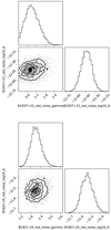 |
Fig. 4. Results of two-dimensional search for Bayesian factors for PSR B1937+21 and PSR B1821-24. |
We find strong evidence for the presence of red noise in both PSR B1937+21 and PSR B1821-24 using 7.3 years of NICER data, with Bayesian factors of 19.182 ± 1.213 and 257.617 ± 1.188, respectively. For PSR B1937+21, the median value of log10A is −12.439 with an uncertainty range of [ − 0.082, +0.081], while the spectral index γ has a median of 0.884 with an uncertainty range of [ − 0.433, +0.508]. Similarly, for PSR B1821-24, the median log10A is −11.527 with an uncertainty range of [ − 0.055, +0.059], and the median γ is 2.121 with an uncertainty range of [ − 0.301, +0.333]. After obtaining evidence of the presence of red noise, extracting it from the timing data becomes a critical step in generating ensemble residuals. To achieve this, we employed the previously introduced harmonic fitting method for red noise extraction, as shown in Figure 5.
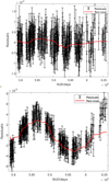 |
Fig. 5. Red noise extracted from PSR B1937+21 and PSR B1821-24 using harmonic fitting method. |
The harmonic fitting method used to extract red noise contains some high-frequency components, which leads to less smooth results. To address this, we applied a low-pass filter to remove signals with frequencies greater than 0.5 years, which resulted in a smoother reconstruction that successfully captured the fluctuations of the timing residuals across the entire observation period. However, slight discrepancies remained at both ends of the time series. These discrepancies are due to edge effects caused by the finite duration of the observation period, which limits the accuracy of the red noise reconstruction at the start and end of the data. The red noise amplitude for PSR B1937 is ±3 μs, while for PSR B1821 it is ±20 μs, differing by an order of magnitude.
We acknowledge that the red noise estimation for B1937, as illustrated in Figure 5, remains marginal relative to the dominant white noise component. Our analysis benefits from 3.8 additional years of data. Specifically, our dataset spans 7.3 years, in contrast to the 3.5 years used in Hazboun et al. (2022). Nevertheless, we recognize that the conclusions presented by Hazboun et al. (2022) remain fundamentally valid. Their results, which are derived from simulations informed by real observational data, constitute a credible and important benchmark. Although our analysis provides a reasonable estimate of the red noise in B1937, further observational data is required to more precisely characterize and confirm its presence.
After removing the extracted red noise, we fitted the remaining low-frequency signals containing clock errors and calculated the white noise amplitudes, with standard deviations of σB1937 = 4.17 μs and σB1821 = 25.07 μs, to simulate the generation of the residuals.
4.2. Single pulsar timing stability analysis
Presently, two notable issues plague the calculation methods for pulsar stability. Firstly, the reliability of stability calculations using the σz method diminishes at the last data point, which corresponds to the longest observation time. This issue arises because only one set of determined timing residuals is utilized at this juncture, thereby introducing uncertainty. Secondly, the calculation of stability error bars is fundamentally limited, as it relies solely on the distribution of observed timing residuals, which lacks theoretical and practical significance. Consequently, incorporating the uncertainty of timing residuals into simulations and repeating the calculations enabled us to derive statistically validated stability metrics and error bars. This approach emphasizes that more meaningful stability assessments can be derived from larger sample statistics. Figure 6 depicts the stability results derived from 500 Monte Carlo simulations using 7.3 years of NICER data from two pulsars. In this context, σz stability is derived from the average of 500 Monte Carlo experiments, with the error bars obtained from the standard deviation. The stability values at different timescales are summarized in Tables 4 and 5.
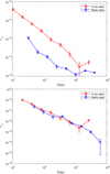 |
Fig. 6. Pulsar stability of PSR B1937+21 and PSR B1821-24. (a) Stability analysis using NICER and NANOGrav data for PSR B1937+21. (b) Stability analysis of PSR B1821-24 using NICER data and PPTA data. |
Stability values for PSR B1937+21 at different timescales.
Stability values for PSR B1821–24 at different timescales.
Pulsar stability serves as a metric for gauging the variance in a pulsar’s rotational frequency fluctuations. Ideally, the stability derived from observations in both the X-ray and radio bands should be consistent when disregarding any errors. However, constrained by factors such as limited detector size and X-ray flux, the measurement uncertainties in the X-ray band notably exceed those in the radio band. Consequently, in the short term, X-ray stability is inferior to that derived from radio observations. Nonetheless, as observation time increases, the impact of observational uncertainties on stability gradually diminishes, with red noise emerging as the primary factor that influences stability calculations. Consequently, over extended observation periods, the stability derived from X-ray and radio observations closely aligns, with the long-term stability in X-rays potentially even surpassing that of radio data, owing to the sensitivity of the σz method for timing red noise. From this perspective, utilizing X-ray timing observations for stability calculations holds significant implications for the long-term assessment of stability. In 2019, Deneva analyzed the one-year NICER data stability of PSR B1937+21 and PSR B1821-24. Due to the limited amount of observational data, the author fitted the stability curve and obtained fitted results of one-year stability for these two pulsars, with values of approximately 1.5 × 10⁻¹³ and 6.5 × 10⁻¹³, respectively, which are close to the results presented in this study (Deneva et al. 2019).
4.3. Ensemble pulsar timing stability analysis
When observational data contain gaps, cubic spline interpolation shows significant fluctuations and distortions, and thereby fails to accurately reflect the true trends and variations. To address these issues, we proposed a new framework for generating ensemble residuals that reliably produces stable timing residuals. We compared the results of cubic spline interpolation with those obtained from the proposed framework for 7.3 years of NICER data for PSR B1937+21, as depicted in Figure 7. We observe that the simulated residuals generated by our framework exhibit a distribution range consistent with the observed residuals (±10 μs), whereas the traditional method (the cubic spline interpolation method) introduces significant errors in observation gaps, with residuals reaching up to 150 μs. Additionally, we proposed an enhanced Wiener filtering algorithm tailored for X-ray data, and the resulting timing residuals are shown in Figure 8. The standard deviation values of the two pulsars decreased significantly after applying the enhanced Wiener filtering, with PSR B1937 reducing from 3.68 μs to 2.31 μs and PSR B1821 reducing from 21.61 μs to 17.00 μs.
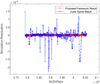 |
Fig. 7. Comparison of simulated timing residuals from the traditional cubic spline method and the proposed framework using 7.3 years NICER observations of PSR B1937+21. |
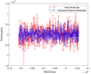 |
Fig. 8. Timing residuals of PSR B1937+21 before (red) and after (blue) applying the enhanced Wiener filtering algorithm. |
We applied the proposed framework to conduct 500 Monte Carlo simulations, and generated simulated timing residuals based on 7.3 years of NICER data for the two pulsars. We then used the long-term timing residuals of the two pulsars to compare the ensemble pulsar stability obtained through the classical weighted method, Wiener filtering method, wavelet decomposition method, and enhanced Wiener filtering method, as illustrated in Figure 9. The stability of the four ensemble pulsar timing algorithms over various observation periods is presented in Table 6. The enhanced Wiener filtering algorithm exhibits its effectiveness in mitigating white noise from X-ray pulsar timing data, thereby elevating stability. Over a 7.3-year timescale, the stability achieved with the enhanced Wiener filtering method exceeds that of the conventional methods by an order of magnitude. These results suggest that the method used significantly enhances the timing stability of X-ray pulsars.
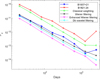 |
Fig. 9. Ensemble pulsar stability calculated by using the four algorithms. |
Stability of four ensemble pulsar timing algorithms across different observation durations.
5. Conclusions and discussion
In this study, we establish X-ray pulsar timing scales using 7.3 years of NICER observation data from PSR B1937+21 and PSR B1821-24, with stability values of 5.21 × 10⁻¹⁴ and 1.14 × 10⁻¹², respectively. By proposing a framework to generate simulated timing residuals, we provided a robust and precise evaluation of the long-term stability for X-ray ensemble pulsar timing. Addressing the prominent presence of white noise in X-ray pulsar timing residuals, we introduced a mirror-symmetric Wiener filtering method based on the Levinson-Durbin iteration technique. This approach comprehensively surpasses all other methods, and achieves the best stability over a 7.3-year period, with a precision of 4.19 × 10⁻¹⁵. Indeed, stability estimators already account for white noise by incorporating more samples over longer lags, thus averaging down the white noise. Using the enhanced Wiener method to reduce white noise may result in a “double averaging” issue. This practice might result in stability comparisons that lack practical significance when contrasted with other comprehensive methods that do not employ such averaging. However, in practical applications, particularly when using pulsar timing for atomic clock calibration, the optimal time-domain Wiener filter can play a significant role. It can enhance calibration accuracy by effectively reducing noise components that are not related to the true signal, thus providing a cleaner and more precise signal for calibration purposes.
The X-ray data exhibit closer consistency with intrinsic noise because they are immune to the propagation effects of the interstellar medium that are contingent on radio-frequency dependence. Hazboun et al. detected red noise in PSR B1821+24 using 3.5 years of NICER observation data. They also predicted that with an observation time of five years and a TOA error of 5 μs, the red noise in pulsar timing can be observed from PSR B1937+21 (Hazboun et al. 2022). In this study, we provided strong evidence for detecting red noise in both PSR B1937+21 and PSR B1821+24 using 7.3 years of NICER observation data. We adopt the approach of fitting harmonic components and successfully reconstruct the red noise time-domain signals of the two pulsars.
Due to certain constraints, such as low radiation flux and limited detection area, the precision of X-ray TOAs is typically one to two orders of magnitude lower than that of radio TOAs, which results in a distinct manifestation of white noise within the X-ray timing residuals. Nevertheless, by utilizing the extraction technique of red noise, it is feasible to extract red noise out of the dominant white noise component. The magnitude of the extracted red noise is consistent with what existed in radio observations (since the X-ray and radio data do not correspond in time, we can only compare the magnitude of the red noise components). Furthermore, we believe that the red noise extracted from long-term X-ray timing residuals is unaffected by interstellar medium noise (Hazboun et al. 2022). When conducting X-ray and radio observations within the same time period, we can compare the trends of red noise in both X-ray and radio spectral bands to confirm whether there is any remaining low-frequency noise in the radio observations (caused by atmospheric dispersion and interstellar medium). This cross-comparison facilitates the understanding and potential correction of any such type of additional noise sources in the radio observations.
It is evident that the long-term stability of pulsar timing may be comparable to or even better than atomic time, whereas the short-term stability of ensemble pulsar timing is significantly lower due to the larger measurement errors in pulsar TOAs. Based on the results obtained in this study for these two pulsars, the one-month stability of ensemble pulsar timing approximates 5.5 × 10⁻¹² order of magnitude. In contrast, some commercial Cesium (Cs) clocks can achieve a one-month stability of 1 × 10⁻¹⁴ order of magnitude, and high-performance optical clocks can even reach a one-month stability of 1 × 10⁻¹⁶ order of magnitude (Hartnett & Luiten 2010). Integrating pulsar timing with existing high-precision atomic time poses tremendous challenges. However, it has been demonstrated that the observations from multiple pulsars can not only be used to detect significant errors in TT (BIPM17) (Hobbs et al. 2012), but to monitor and calibrate atomic clock jumps (Hartnett & Luiten 2010). Although pulsar-based timescales are unlikely to make significant contributions to the stability of atomic timescales in the coming ten years, they will be serving as a valuable independent means for verifying atomic timescales (Hobbs et al. 2012).
Identifying pulsars that exhibit high stability in both the radio and X-ray bands is highly valuable and will serve as one of our future research directions. Future space X-ray observation projects are expected to see improvements in both detection sensitivity and observational coverage, which will contribute to obtaining higher-quality datasets. Projects such as eXTP (Zhang et al. 2016) and STROBE-X (Wilson-Hodge et al. 2017), with their advanced detection capabilities and high temporal and spectral resolution, are expected to greatly enhance X-ray pulsar timing precision. With the deployment of these high-performance X-ray detectors, the precision of X-ray pulse TOA measurements will continue to improve. By designing more precise pulsar timing filtering algorithms, there is huge potential to further advance the applications of pulsar timing in fields such as atomic time error correction and solar system ephemeris refinement.
Acknowledgments
This work was supported by the National Natural Science Foundation of China No. 62103313. This research utilized the data obtained from the NICER Data Archive and software resources made available by the High Energy Astrophysics Science Archive Research Center (HEASARC).
References
- Alam, M. F., Arzoumanian, Z., Baker, P. T., et al. 2020, ApJS, 252, 4 [NASA ADS] [CrossRef] [Google Scholar]
- Allan, D. W. 1987, in 41st Annual Symposium on Frequency Control, 2, https://doi.org/10.1109/FREQ.1987.200994 [CrossRef] [Google Scholar]
- Arzoumanian, Z., Brazier, A., Burke-Spolaor, S., et al. 2018, ApJS, 235, 37 [CrossRef] [Google Scholar]
- Backer, D. C., Kulkarni, S. R., Heiles, C., et al. 1982, Nature, 300, 615 [NASA ADS] [CrossRef] [Google Scholar]
- Bogdanov, S. 2017, Proc. IAU, 13, 116 [Google Scholar]
- Chen, S., Caballero, R. N., Guo, Y. J., et al. 2021, MNRAS, 508, 4970 [NASA ADS] [CrossRef] [Google Scholar]
- Cognard, I., Bourgois, G., Lestrade, J. F., et al. 1996, A&A, 311, 179 [Google Scholar]
- Deneva, J. S., Ray, P. S., Lommen, A., et al. 2019, ApJ, 874, 160 [Google Scholar]
- Desvignes, G., Caballero, R. N., Lentati, L., et al. 2016, MNRAS, 458, 3341 [Google Scholar]
- Edwards, R. T., Hobbs, G. B., & Manchester, R. N. 2006, MNRAS, 372, 1549 [Google Scholar]
- Ellis, J. A., Vallisneri, M., Taylor, S. R., & Baker, P. T. 2019, Astrophysics Source Code Library [record ascl:1912.015] [Google Scholar]
- EPTA Collaboration (Antoniadis, J., et al.) 2023, A&A, 678, A48 [Google Scholar]
- Fairhead, L., & Bretagnon, P. 1990, A&A, 229, 240 [NASA ADS] [Google Scholar]
- Foster, R. S., & Backer, D. C. 1990, ApJ, 361, 300 [NASA ADS] [CrossRef] [Google Scholar]
- Gendreau, K., & Arzoumanian, Z. 2017, Nat. Astron., 1, 895 [NASA ADS] [CrossRef] [Google Scholar]
- Gendreau, K. C., Arzoumanian, Z., Adkins, W., et al. 2016, Proc. SPIE, 9905, 99051 [Google Scholar]
- Hartnett, J. G., & Luiten, A. N. 2010, Rev. Mod. Phys., 83, 184 [Google Scholar]
- Hazboun, J. S., Crump, J., Lommen, A. N., et al. 2022, ApJ, 928, 67 [NASA ADS] [CrossRef] [Google Scholar]
- Hobbs, G., Archibald, A., Arzoumanian, Z., et al. 2010, Class. Quantum Gravity, 27, 084013 [Google Scholar]
- Hobbs, G., Coles, W., Manchester, R. N., et al. 2012, MNRAS, 427, 2780 [NASA ADS] [CrossRef] [Google Scholar]
- Hobbs, G., Guo, L., Caballero, R. N., et al. 2020, MNRAS, 491, 5951 [Google Scholar]
- Jenet, F. A., Hobbs, G. B., Lee, K. J., & Manchester, R. N. 2005, ApJ, 625, L123 [NASA ADS] [CrossRef] [Google Scholar]
- Johnston, S., Karastergiou, A., Keith, M. J., et al. 2020, MNRAS, 493, 3608 [NASA ADS] [CrossRef] [Google Scholar]
- Kaspi, V. M. 1995, ASP Conf. Ser., 72, 345 [Google Scholar]
- Kaspi, V. M., Taylor, J. H., & Ryba, M. F. 1994, ApJ, 428, 713 [NASA ADS] [CrossRef] [Google Scholar]
- Kawai, N., Tamura, K., & Saito, Y. 1998, Adv. Space Res., 21, 213 [Google Scholar]
- Lee, K. J., Bassa, C. G., Janssen, G. H., et al. 2012, MNRAS, 423, 2642 [NASA ADS] [CrossRef] [Google Scholar]
- Li, Z. X., Lee, K. J., Caballero, R. N., et al. 2020, Sci. China Phys. Mech. Astron., 63, 219512 [Google Scholar]
- Lyne, A. G. 1987, Nature, 328, 399 [NASA ADS] [CrossRef] [Google Scholar]
- Manchester, R. N. 2013, Class. Quantum Gravity, 30, 55 [Google Scholar]
- Miles, M. T., Shannon, R. M., Bailes, M., et al. 2022, MNRAS, 519, 3976 [Google Scholar]
- Paul, A., Susobhanan, A., Gopakumar, A., et al. 2019, in 2019 URSI Asia-Pacific Radio Science Conference (AP-RASC), https://doi.org/10.23919/URSIAP-RASC.2019.8738505 [Google Scholar]
- Perera, B. B. P., DeCesar, M. E., Demorest, P. B., et al. 2019, MNRAS, 490, 4666 [Google Scholar]
- Petit, G. 1996, A&A, 308, 290 [Google Scholar]
- Petit, G., Thomas, C., & Tavella, P. 1993, in 24th Annual Precise Time and Time Interval (PTTI) Applications and Planning Meeting, in NASA, 73 [Google Scholar]
- Prigozhin, G., Gendreau, K., Doty, J. P., et al. 2016, Proc. SPIE, 9905, 436 [Google Scholar]
- Rasmussen, C. E., & Williams, C. K. I. 2006, Gaussian Processes for Machine Learning (Cambridge, MA: MIT Press) [Google Scholar]
- Reardon, D. J., Shannon, R. M., Cameron, A. D., et al. 2021, MNRAS, 507, 2137 [CrossRef] [Google Scholar]
- Rodin, A. E. 2008, MNRAS, 387, 1583 [Google Scholar]
- Rodin, A. E., & Fedorova, V. A. 2018, Astron. Rep., 62, 378 [Google Scholar]
- Spiewak, R., Bailes, M., Miles, M. T., et al. 2022, Pub. Astron. Soc. Australia, 39, e027 [Google Scholar]
- Srivastava, A., Desai, S., Kolhe, N., et al. 2023, PRD, 108, 023008 [Google Scholar]
- Sun, H. F., Yao, D. K., Shen, L. R., et al. 2023, Acta Astronaut., 210, 141 [Google Scholar]
- Tarafdar, P., Nobleson, K., Rana, P., et al. 2022, Pub. Astron. Soc. Australia, 39, e053 [Google Scholar]
- Taylor, J. H. 1991, Proc. IEEE, 79, 1054 [Google Scholar]
- The NANOGrav Collaboration (Arzoumanian, Z., et al.) 2019, ApJ, 813, 65 [Google Scholar]
- Verbiest, J. P. W., Lentati, L., Hobbs, G., et al. 2016, MNRAS, 458, 1267 [Google Scholar]
- Vivekanand, M. 2019, ApJ, 890, 143 [Google Scholar]
- Weisberg, J. M., & Taylor, J. H. 1981, Gen. Relativ. Gravit., 13, 1 [Google Scholar]
- Wilson-Hodge, C. A., Ray, P. S., Gendreau, K., et al. 2017, Results Phys., 7, 3704 [Google Scholar]
- Xu, H., Chen, S., Guo, Y., et al. 2023, Res. Astron. Astrophys., 23, 075024 [CrossRef] [Google Scholar]
- Zhang, S. N., Feroci, M., Santangelo, A., et al. 2016, SPIE Conf. Ser., 9905 [Google Scholar]
- Zhao, C. S., Zhu, X. Z., & Zhou, Z. R. 2023, JTF, 46, 188 [Google Scholar]
- Zharov, V. E., Oreshko, V. V., Potapov, V. A., et al. 2019, Astron. Rep., 63, 112 [Google Scholar]
- Zhong, C. X., & Yang, T. G. 2007, JUCAS, 806 [Google Scholar]
- Zhong, C. X., & Yang, T. G. 2007, Acta Phys. Sin., 56, 6157 [Google Scholar]
- Zhou, Q. Y., Wei, Z. Q., Yan, L. L., et al. 2021, Acta Phys. Sin., 70, 13 [Google Scholar]
- Zhou, Q. Y., Wei, Z. Q., Zhang, H., et al. 2021, Acta Astron. Sin., 62, 88 [Google Scholar]
All Tables
Bayes factors for the detection of red noise, along with the corresponding values of amplitude log10A and spectral index γ.
Stability of four ensemble pulsar timing algorithms across different observation durations.
All Figures
|
Fig. 1. Timing residuals after fitting the timing model: (a) PSR B1937+21, (b) PSR B1821-24. |
| In the text | |
|
Fig. 2. Radio timing residuals for PSR B1937+21 and PSR B1821-24. (a) PSR B1937+21, (b) PSR B1821-24. |
| In the text | |
|
Fig. 3. Framework for generating ensemble pulsar timing residuals. |
| In the text | |
|
Fig. 4. Results of two-dimensional search for Bayesian factors for PSR B1937+21 and PSR B1821-24. |
| In the text | |
|
Fig. 5. Red noise extracted from PSR B1937+21 and PSR B1821-24 using harmonic fitting method. |
| In the text | |
|
Fig. 6. Pulsar stability of PSR B1937+21 and PSR B1821-24. (a) Stability analysis using NICER and NANOGrav data for PSR B1937+21. (b) Stability analysis of PSR B1821-24 using NICER data and PPTA data. |
| In the text | |
|
Fig. 7. Comparison of simulated timing residuals from the traditional cubic spline method and the proposed framework using 7.3 years NICER observations of PSR B1937+21. |
| In the text | |
|
Fig. 8. Timing residuals of PSR B1937+21 before (red) and after (blue) applying the enhanced Wiener filtering algorithm. |
| In the text | |
|
Fig. 9. Ensemble pulsar stability calculated by using the four algorithms. |
| In the text | |
Current usage metrics show cumulative count of Article Views (full-text article views including HTML views, PDF and ePub downloads, according to the available data) and Abstracts Views on Vision4Press platform.
Data correspond to usage on the plateform after 2015. The current usage metrics is available 48-96 hours after online publication and is updated daily on week days.
Initial download of the metrics may take a while.