| Issue |
A&A
Volume 697, May 2025
|
|
|---|---|---|
| Article Number | L8 | |
| Number of page(s) | 6 | |
| Section | Letters to the Editor | |
| DOI | https://doi.org/10.1051/0004-6361/202554427 | |
| Published online | 15 May 2025 | |
Letter to the Editor
The tidal heating of the exoplanet 55 Cnc e
The role of the orbital eccentricity
1
Instituto de Astronomia, Geofísica e Ciências Atmosféricas, Universidade de São Paulo, São Paulo, Brazil
2
Instituto de Astronomía Teórica y Experimental, Observatorio Astronómico, Universidad Nacional de Córdoba, Córdoba, Argentina
⋆ Corresponding author: This email address is being protected from spambots. You need JavaScript enabled to view it.
Received:
8
March
2025
Accepted:
22
April
2025
Abstract
Context. Observations with warm Spitzer and JWST have revealed a high and variable brightness in the planet 55 Cnc e.
Aims. Our aim is to make an inventory of the tidal effects on the rotational and orbital evolution of the planet 55 Cnc e enhanced by the nonzero orbital eccentricity.
Methods. The creep-tide theory is used in simulations and dynamical analyses that explore the difficult trapping of the planet’s rotation in a 3:2 spin-orbit resonance and the most probable synchronization of the rotation.
Results. The strong tidal dissipation of energy, enhanced by the nonzero orbital eccentricity, may explain the observed brightness anomalies. However, the strong dissipation should also circularize the orbit. The observed nonzero eccentricity, if true, would indicate that an unknown planet in a close orbital resonance with 55 Cnc e perturbing the motion of this planet should exist.
Key words: planets and satellites: dynamical evolution and stability / planets and satellites: individual: 55 Cnc e
© The Authors 2025
 Open Access article, published by EDP Sciences, under the terms of the Creative Commons Attribution License (https://creativecommons.org/licenses/by/4.0), which permits unrestricted use, distribution, and reproduction in any medium, provided the original work is properly cited.
This article is published in open access under the Subscribe to Open model. This email address is being protected from spambots. You need JavaScript enabled to view it. to support open access publication.
1. Introduction
This paper inventories the tidal effects on the rotational and orbital evolution of the planet 55 Cnc e. This planet has been the object of recent observations with warm Spitzer and JWST that revealed a high and variable brightness (Demory et al. 2016; Patel et al. 2024). This planet lies in an orbit very close to a solar-like host star and belongs to a non-compact system including four other planets. We discuss the dynamics of trapping the planet rotation in a 3:2 spin-orbit resonance and the more common alternative in which the rotation is synchronized with the orbital motion. We discuss the observed nonzero eccentricity of the system. The fast circularization of any isolated ultrashort-period orbit in a few million years and the system’s old age led us to think that the observed eccentricity, if true, is being forced by an unknown twin planet in a close orbital resonance with 55 Cnc e.
The creep-tide theory was chosen for this study because it does not introduce ad hoc models, has only one free parameter, and is valid for both gaseous and rocky bodies. The creep-tide theory arises from interpreting the matter displacements inside the body as a smooth radial flow without turbulence (low-Reynolds-number flow); namely, a Newtonian creep. The basic creep equation used to establish the theory is an approximate solution of the Navier-Stokes equation (Ferraz-Mello 2013). However, the results shown in this paper are not exclusive to the creep-tide theory. They could also be obtained with the classical Darwinian theories, provided that appropriate ad hoc models were chosen to relate tidal lags and frequencies.
2. Orbital evolution of a synchronized planet
We first study the system’s evolution, assuming that the planetary rotation is synchronized. We consider that there are no other constraints and show that because of the tide on the planet, the orbital eccentricity is rapidly damped to zero (Fig. 1). We show the curves corresponding to three different values of the planet’s relaxation factor, the largest of which, γ = 2 × 10⁻⁷ s−1, is the value often adopted in the study of the solid Earth (see Ferraz-Mello 2013). The other values shown correspond to harder bodies. We do not consider cases of a softer planet; in these cases, the damping is faster than the ones shown. After the eccentricity is damped, the stellar tide dominates, and the planet falls toward the star. The fall on the star will occur in no more than 1 Gyr. The remaining lifetime depends on the star’s relaxation factor. The adopted factors of γs = 50, 100, 200 s−1 are based on the results of previous studies on the evolution of the rotation of host stars of the spectral types G7 – K0 with large close-in companions (Ferraz-Mello 2015).
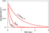 |
Fig. 1. Evolution of the planet’s orbital eccentricity in synchronous rotation. The labels indicate the planet’s relaxation factor. e(t = 0) = 0.028. |
To complete this study, we show the evolution of the synchronous planet under the hypothesis that the observed eccentricity is forced by a third-body perturbation and so is not tidally damped (Fig. 3). In this case, the tides on the planet are dominant and responsible for the fall of the planet in a much shorter time, less than 25 Myr. The stellar tide has only a small influence – the curves shown are the superposition of the solutions corresponding to three different values of the stellar relaxation factor (the same appearing in Fig. 2). The faster-falling case corresponds to a softer planet with γ = 7 × 10⁻⁷ s−1 and was introduced to complete the range of values of γ used for the solid Earth (see Ferraz-Mello 2013). This solution would correspond to a decrease in the orbital period of 10−7 d per year. This value is one order of magnitude smaller than the current precision of the period determinations.
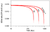 |
Fig. 2. Evolution of the system with the planetary rotation synchronized with the orbital motion. The labels indicate the stellar tide relaxation factor. The planetary tide effect is negligible. |
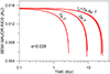 |
Fig. 3. Evolution of the system with the planet rotation synchronized when the eccentricity is kept fixed at e = 0.028. The labels show the planetary relaxation factor. Each line is a bundle of three solutions corresponding to the stellar relaxation factors 50, 100, and 200 s−1. |
The interplay of the importance of the two tides in the above results may be understood by looking at the leading terms in the expressions of their contributions to the evolution of the semimajor axis. When the planet’s rotation is assumed to be synchronous and the star is assumed to have a slow rotation, they are
 (1)
(1)
and
 (2)
(2)
where the subscripts s and p indicate star and planet, respectively (Ferraz-Mello 2013, 2022). The notations used are the usual ones: m is mass, R is the radius, a is the semimajor axis, n is the mean motion, e is eccentricity, and k is the fluid Love number.
The ratio of the contributions of the two tides to the fall of the planet is given by
 (3)
(3)
where 𝕂 is a positive number of order  . The coefficient of e2 in Eq. (3) is much larger than 1 and compensates for the smallness of e2, which makes the component due to the planetary tide dominate the variation in a. However, when e → 0, this dominance ceases and the evolution becomes dominated by the stellar tide (as is seen in Fig. 2).
3. Orbital evolution of a planet initially in the 3:2 spin-orbit resonance
We repeat here the previous analysis but assume that the planet’s rotation is initially trapped in the 3:2 resonance.
Figures 4 and 5 show rapid damping of the eccentricity and escape from the 3:2 spin-orbit resonance. We see two different phases in this process. First, the eccentricity is quickly damped to a small value. When the decreasing eccentricity reaches the critical value corresponding to the spin-orbit resonance (see Appendix A.1), the stable stationary solution ceases to exist, and the rotation escapes the resonance and is slowly driven to synchronization. This phase lasts a few thousand years.
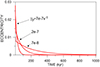 |
Fig. 4. Evolution of the orbital eccentricity of the planet initially in 3:2 spin-orbit resonance. The labels indicate the planet’s relaxation factor. |
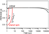 |
Fig. 5. Evolution of the system with the planet rotation initially in 3:2 spin-orbit resonance for two different values of the planet’s relaxation factor. The eccentricity is damped, and the rotation tends to be synchronous (the red and black curves merge). |
We note that, in this phase, the orbital period is increasing; that is,  . We recall that the contribution of the planetary tide to the variation in the semimajor axis when the planet’s rotation is faster than the orbital motion is positive and, in the first approximation, independent of the eccentricity:
 (4)
(4)
where νp = 2(Ωp − n) is the so-called semidiurnal frequency. This equation is not enough to understand the cases in the 3:2 spin-orbit resonance, but it applies to what is seen in the first thousand years of Fig. 5 because the planet escapes the resonance and the eccentricity decreases quickly. Otherwise, a more complete expression is necessary (see Appendix B).
As before, to complete the study, we consider the evolution of the system when the planetary rotation is forced to remain in the 3:2 spin-orbit resonance and the observed eccentricity is forced by a third-body perturbation and not damped by the tides. In this case, the planet eventually falls on the star in a timescale of a few hundred million years. The evolution is dominated by the planetary tides but the simple approximation given by Eq. (4) is not enough to understand the results. This approximation fails in the neighborhood of the 3:2 spin-orbit resonance because of the smallness of (νp − n) in this neighborhood (see Appendix B).
In these cases, the period decay is much faster than in the case of a synchronous planet. When the solution is forced to remain in the 3:2 spin-orbit resonance and γ = 2 × 10⁻⁷ s−1, we have a decrease in the orbital period of ∼3 × 10⁻⁶ d per year. This value is of the same order of magnitude as the current precision of the period determinations and, if true, could be detected. We recall that  is proportional to the planetary relaxation factor, and thus a softer planet, with a larger relaxation factor, would be on the detection level.
4. Heat dissipation
The above results do not appear to favor the existence of a planet in a nonzero eccentricity orbit so close to the star. We either have a planet whose eccentricity is quickly damped to zero or a forced eccentricity accelerating the planet’s fall onto the star. In that case, orbital energy is being lost by the system. If we neglect the variations in the planet’s geometry, the time derivatives in the orbital and rotational energies are given by:
 (5)
(5)
(Ip is the axial moment of inertia of the planet and Ωp its rotation velocity).
The variations can be determined from the quantities, Ṗ, obtained from the results shown in Figs. 5 and 6. As was discussed in previous sections, the planetary tide is dominant when the eccentricity is forced to remain constant, and so the planet is the body responsible for the orbital energy loss.
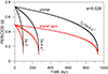 |
Fig. 6. Evolution of the system with the planet rotation forced to remain in the 3:2 spin-orbit resonance and the orbital eccentricity kept fixed at e = 0.028. The labels show the planetary relaxation factor. |
In intermediate cases, corresponding to an Earth-like relaxation factor (2 × 10⁻⁷ s−1), we obtain, in the case of a synchronous rotation,

The mechanical energy lost is liberated within the planet and might flow through its surface at a rate of ∼0.5 Mw/m2. The amount of energy used to accelerate the planet’s rotation is only a negligible fraction of it.
This value is much larger than in any other reported case. It is worth noting that if we use the formula for tidal heating based on the classical Darwin theory (see Barnes et al. 2009) and the quality factor Q = 500, in the middle of the range accepted for the solid Earth, we obtain 0.45 Mw/m2. Quick et al. (2020) also report a similar value. If the planet’s rotation is trapped in the 3:2 resonance, this result is 100 times larger.
In general, the energy lost by the orbit may contribute to the heat release in both the star and the planet. In this case, calculations have shown that the variation in  is due to the planetary tide.
The above results favor widespread volcanic activity, as has been suggested by Winn et al. (2018), to explain the large irregular brightness on the dayside of the planet observed with Spitzer (Demory et al. 2016). If confirmed, it would explain the brightness anomalies by way of an intense volcanism of tidal origin and an incandescent planet.
5. Consequences of a lower eccentricity
There is not much we can do to get less dissipation on the planet. We need a slower orbital decay to reduce the dissipation. For example, we can assume a relaxation factor smaller than the chosen one. However, this goes in the opposite direction to what we should expect. If the planet is hot, the fluidity may be greater, and consequently, the relaxation factor and the dissipation are expected to be larger.
We can change the eccentricity. The nominal value has a large error bar: 0.028 ± 0.018. The minimum value in the 1σ confidence domain is e = 0.01. With this lower eccentricity, no capture in the 3:2 spin-orbit resonance is possible, and synchronous rotation is the only possibility. Repeating what was done in Sect. 2, we obtain Fig. 7.
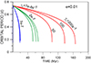 |
Fig. 7. Evolution of the system with the planet rotation synchronized with the orbital motion, for a fixed eccentricity at e = 0.1 and relaxation factors, as is indicated by the labels. The same colors indicate solutions corresponding to the same planetary relaxation factor. Each bundle contains solutions corresponding to three different stellar relaxation factors. |
Since the eccentricity is smaller, the contribution of the planetary tide is not as dominant as when e = 0.028. It still dominates the evolution, but the stellar tide also contributes. Then, for each planetary relaxation factor, we see three lines in the plot corresponding to the stellar relaxation factors 50, 100, and 200 s−1.
The decrease in the period when γp = 2 × 10⁻⁷ s−1 is 3.5 × 10⁻⁹ d per year. The overall heat dissipation is now smaller than before but still large: 70 kw/m2.
6. The forced eccentricity
The last figure was made assuming that the observed eccentricity is forced and, therefore, cannot be damped by the tidal torques. This hypothesis arises from the fact that, otherwise, the orbit of 55 Cnc e would be rapidly circularized. We are maybe looking at this 10-Gyr-old system just when this final fast circularization occurs. However, it is more likely that this eccentricity results from perturbations by other bodies. The known planets cannot produce an eccentricity of 0.028 or even 0.01. The maximum evection-like perturbations found are thousands of times smaller. The same is true for the perturbations due to the star companion 55 Cnc B. Since tides do not allow an eccentricity to remain unaltered in a planet so close to the host star as 55 Cnc e, we are forced to assume that an unknown body is producing them.
We can, for instance, assume that it is located in the large gap between 55 Cnc e and its closest sibling, the hot Jupiter 55 Cnc b. The calculations can follow the same recipe used to study the forced eccentricity of LP 791-18 d (Ferraz-Mello et al. 2025). They show that a twin planet, with the same mass as 55 Cnc e, cannot produce a forced eccentricity in the confidence interval of the observed eccentricity unless it is in a close resonance with 55 Cnc e as the 2:1 or 3:2 period resonances. Outside these resonances, it cannot produce the observed eccentricity. Unfortunately, there is no known way to detect such a planet. The TTVs due to such a companion would be too small to be observed: only 1 second.
The other possibility is that this planet had a close approach to another body, in a higher orbit, and had its eccentricity excited by the encounter. If so, all simulations show that the orbit circularizes rapidly. This encounter should have occurred no more than 10 or 20 Myr ago. Although unexpected, these encounters are not rare.
Finally, the actual eccentricity may be closer to zero than the adopted value. The compatibility of circularization with the observations is in the 2σ range. Since  is proportional to e2, the planet’s tidal dissipation would vanish, and the strong irradiation on the planet should explain the observed phenomena. However, all other determinations (Baluev 2015; Bourrier et al. 2018; Rosenthal et al. 2021) give values that are even larger than the value e = 0.028 determined by Nelson et al. (2014).
7. Conclusion
This paper has inventoried the tidal dynamics of planet 55 Cnc e, searching for facts that may help us to understand the large brightness irregularities observed by warm Spitzer and JWST (Demory et al. 2016; Patel et al. 2024). The first point examined was the possibility of a capture of the rotation in a 3:2 spin-orbit resonance. With a nominal eccentricity of 0.028, this possibility exists. However, this is not a robust situation. The eccentricity is strongly affected by the planetary tides and decreases quickly, leading the planetary rotation to soon escape from the 3:2 resonance and be synchronized. After synchronization and circularization, the planetary tide ceases to dominate the system’s evolution, and the weaker stellar tide becomes dominant. The planet may remain orbiting the star for some hundred million years, the exact remaining time until the fall being dependent on the stellar relaxation factor (Fig. 2).
The only way to avoid rapid circularization of the orbit is the eccentricity being forced by a third body. However, the other planets in the system are far away and cannot force an eccentricity larger than a few thousandths. If so, this third body must be an unknown one. But almost all initial conditions between 55 Cnc e and its closest sibling lead to rapid circularization. The only exceptions occur if the third body is assumed to be very close to the 2:1 or 3:2 period resonances with 55 Cnc e.
The presence of a forced eccentricity means that circularization of the orbit did not happen. However, the planet is too close to the star, and the forced eccentricity contributes to increasing the effects of the planetary tide and accelerates the star’s rate of fall toward the star. All calculations show that this planet is falling onto the star in, at most, some hundreds of millions of years.
The orbital energy decreases quickly and may dissipate inside the planet. If the dissipated energy flows through the planet’s surface, it corresponds to many kilowatts per square meter; the actual value depends on the forced eccentricity and the planet’s relaxation factor. Such a high heat flow has not been found in any planet studied before, but it must be normal for planets with nonzero eccentricity so close to a solar-like host star. The volcanism it may induce could be responsible for the irregular brightness observed by warm Spitzer (Winn et al. 2018).
The calculations were done using the creep-tide theory equations expanded up to the sixth power of eccentricities. The simplified formulas included in the text were only used to identify the individual roles of the stellar and planetary tides in each case.
We remind that the relaxation factor γ is inversely proportional to the dynamical viscosity (Darwin 1879; Ferraz-Mello 2013).
Acknowledgments
This investigation was sponsored by CNPq (Proc. 303540/2020-6) and FAPESP (Procs. 2016/13750-6 ref. PLATO mission).
References
- Baluev, R. 2015, MNRAS, 446, 1493 [Google Scholar]
- Barnes, R. 2017, Celest. Mech. Dyn. Astron., 129, 509 [Google Scholar]
- Barnes, R., Jackson, B., Greenberg, R., & Raymond, S. N. 2009, ApJ, 700, L30 [CrossRef] [Google Scholar]
- Bourrier, V., Dumusque, X., Dorn, C., et al. 2018, A&A, 619, A1 [NASA ADS] [CrossRef] [EDP Sciences] [Google Scholar]
- Bouvier, J., Forestini, M., & Allain, S. 1997, A&A, 326, 1023 [NASA ADS] [Google Scholar]
- Callegari, N., & Rodríguez, A. 2013, Celest. Mech. Dyn. Astron., 116, 389 [NASA ADS] [CrossRef] [Google Scholar]
- Celletti, A. 2010, Stability and Chaos in Celestial Mechanics (Heidelberg: Springer) [CrossRef] [Google Scholar]
- Correia, A. C. M., Boué, G., Laskar, J., & Rodríguez, A. 2014, A&A, 571, A50 [NASA ADS] [CrossRef] [EDP Sciences] [Google Scholar]
- Darwin, G. H. 1879, Phil. Trans. R. Soc., 170, 1 [Google Scholar]
- Demory, B. O., Gillon, M., Madhusudhan, N., & Queloz, D. 2016, MNRAS, 455, 2018 [NASA ADS] [CrossRef] [Google Scholar]
- Ferraz-Mello, S. 1979, Dynamics of the Galilean Satellites, (IAG-USP, São Paulo, revised 2022) [Google Scholar]
- Ferraz-Mello, S. 2013, Celest. Mech. Dyn. Astron., 116, 109 [Google Scholar]
- Ferraz-Mello, S. 2015, Celest. Mech. Dyn. Astron., 122, 359 [Google Scholar]
- Ferraz-Mello, S. 2022, Proc. IAU Symp., 364, 20 [Google Scholar]
- Ferraz-Mello, S., Rodríguez, A., & Hussmann, H. 2008, Celest. Mech. Dyn. Astron., 101, 171 [Google Scholar]
- Ferraz-Mello, S., Tadeu dos Santos, M., Folonier, H., et al. 2015, ApJ, 807, 78 [Google Scholar]
- Ferraz-Mello, S., Folonier, H. A., & Gomes, G. O. 2022, Celest. Mech. Dyn. Astron., 134, 25 [Google Scholar]
- Ferraz-Mello, S., Bechara, T. M., & Alves-Silva, R. 2025, Eur. Phys. J. Sp. Top., (submitted) [Google Scholar]
- Nelson, B. E., Ford, E. B., Wright, J. T., et al. 2014, MNRAS, 441, 442 [Google Scholar]
- Patel, J. A., Brandeker, A., Kitzmann, D., et al. 2024, A&A, 690, A159 [NASA ADS] [CrossRef] [EDP Sciences] [Google Scholar]
- Pinzari, G., Scoppola, B., & Veglianti, M. 2024, Celest. Mech. Dyn. Astron., 136, 39 [Google Scholar]
- Quick, L. C., Roberge, A., Mlinar, A. B., & Hedman, M. M. 2020, PASP, 132, 084402 [NASA ADS] [CrossRef] [Google Scholar]
- Rodríguez, A., Callegari, N., Jr, Michtchenko, T. A., & Hussmann, H. 2012, MNRAS, 427, 2239 [NASA ADS] [CrossRef] [Google Scholar]
- Rosenthal, L. J., Fulton, B. J., Hirsch, L. A., et al. 2021, ApJS, 255, 8 [NASA ADS] [CrossRef] [Google Scholar]
- Winn, J. N., Sanchis-Ojeda, R., & Rappaport, S. 2018, New Astr. Rev., 83, 37 [Google Scholar]
Appendix A: Spin-orbit resonance trapping dynamics
Usual studies of spin-orbit resonance consider an asymmetric companion (see Celletti 2010; Callegari & Rodríguez 2013; Pinzari et al. 2024). The equatorial asymmetry is responsible for a force that counterbalances the tidal torques, allowing the rotation of the body to be synchronized with the orbital motion (Ferraz-Mello et al. 2008; Rodríguez et al. 2012). The differential equations are pendulum-like, second-order differential equations. However, if an asymmetry does not exist a priori, the rotational dynamics is rather ruled by a first-order differential equation (Correia et al. 2014; Ferraz-Mello et al. 2015) of the form
 (A.1)
(A.1)
(Ferraz-Mello 2013; Ferraz-Mello et al. 2022) where 𝒜 is a positive coefficient depending on the dynamical parameters of the system, γ is the relaxation factor of the body, n the orbital mean motion, and E2, k known functions of the orbital eccentricity (Cayley coefficients).
Figure A.1 shows the phase plane of Eq. A.1 in one special case chosen for its rich features. In this case, the parameters are those of the system formed by 55 Cnc e and its host star with a planetary relaxation factor γ = 2 × 10⁻⁷ s−1 – a relaxation factor of the order of the solid Earth’s relaxation factor (see (Ferraz-Mello 2013)). The eccentricity was arbitrarily fixed at e = 0.15, a value unrealistic but good to emphasize the main features of the equation.
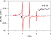 |
Fig. A.1. Phase plane |

The points where the curve crosses the axis  are equilibrium points of the system, a.k.a. stationary solutions of Eq. A.1. When the curve crosses the axis in the descending direction (the derivative of
  is negative), the solution is stable. The velocity is positive on the left of the crossing point 𝕊 and negative on its right (see Fig. A.2). In contrast, the corresponding stationary solution is unstable if the curve is ascending at the crossing point (the derivative of
  is positive).
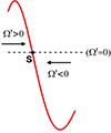 |
Fig. A.2. Stable stationary solution (𝕊). |
In Fig. A.1 one may see 5 stable stationary solutions, at the frequencies  (k = 1, 2, 3, 4, 5). The two corresponding to k = 1 and k = 5 would require a zoom to be seen, but the other three are evident. In its evolution, the planet’s rotation may be trapped in any of these solutions. If the planet starts as a fast rotator, it will evolve from the right to the left and will be trapped in the 5/2 orbital resonance. If, because of a variation in its eccentricity, it succeeds in escaping to this resonance, it will be trapped in the next one. The pseudo-synchronous stationary solution at 𝕊 is the only one for which there is no escape route. We say pseudo-synchronous because the point 𝕊 is not exactly at Ω = n, but slightly at its right (see Ferraz-Mello et al. 2008; Ferraz-Mello 2013).
A.1. The trapping in the 3:2 spin-orbit resonance
Let us now consider the phase plane  of Eq. A.1 in some cases akin to the actual 55 Cnc e. Figure A.3 shows the curve corresponding to the observed eccentricity of 55 Cnc e and three different values for the relaxation factor: γ = 7 × 10⁻⁸ s−1, γ = 2 × 10⁻⁷ s−1, and γ = 7 × 10⁻⁷ s−1. These values are of the same order as the relaxation factor of the solid Earth. The inset on the top of the figure shows that in the softer case (γ = 7 × 10⁻⁷ s−1), the crest at the 3:2 resonance does not cross the dashed line, which means that, in this case, the corresponding stationary solution does not exist. The planet may be trapped in this resonance in the harder cases, but not in the softer ones.
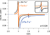 |
Fig. A.3. Phase plane |

No crest appears at Ω = 2n, showing that no other non-synchronous stationary solution exists beyond 3:2 at the current eccentricity of the planet.
In the other two figures (Figs. A.4 and A.5), we discuss the dependence of the trapping on the orbital eccentricities to know the limiting values necessary to have the spin-orbit 3:2 resonance.
Figure A.4 shows the phase diagram for the relaxation factor γ = 2 × 10⁻⁷ s−1 and the eccentricities 0.018, 0.034, and 0.050. We see that in all cases the curves intersect the axis  . When e = 0.018, we would need a zoom to see if it actually crosses the axis or not. But this detail is not important. What matters is that close to e = 0.018 we have the limit necessary for trapping in the stationary 3:2 solution. If, in some instant, because of any perturbations, the eccentricity falls below that limit, the solution will escape the resonance and evolve toward synchronization, and there is no way for it to come back.
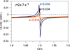 |
Fig. A.4. Phase diagram |

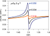 |
Fig. A.5. Same as Fig. A.4 for the case of a larger relaxation factor: γ = 7 × 10⁻⁷ s−1 (a softer planet). |
Fig. A.5 is the same as above for a softer planet1 with γ = 7 × 10⁻⁷ s−1 and the same eccentricities as before. In this case, the lower trapping limit is e ∼ 0.034. With this relaxation factor, the planet’s rotation cannot be trapped in the 3:2 spin-orbit resonance, and the system should have evolved to the pseudo-synchronous solution. Conversely, if we prove that the rotation is trapped in the 3:2 resonance, we may say that the relaxation factor is smaller than 7 × 10⁻⁷ s−1.
It is noteworthy that the limits found in Figs. A.4 and A.5 agree perfectly with the predictions given by the condition
 (A.2)
(A.2)
found by Correia et al. (2014) for the minimum eccentricity necessary for the existence of the stable equilibrium at the 3:2 spin-orbit resonance.
Appendix B: Variation of the semimajor axis
Equation 4 is common to all tidal theories and generally works fine. It may be quickly interpreted when we note that  has the same sign as νp. So
  is positive when Ωp > n, and negative otherwise. The same is true with
  . So, as the Galilean satellites orbit a fast-rotating planet, they recede from it, whereas close-in planets generally orbit slow-rotating stars and thus fall on the star. However, this classical statement is only true if the considered satellites or planets are in almost circular orbits.
Equation 4 is the limit of a more general equation involving eccentricities when e → 0. However, in the vicinity of the 3:2 spin-orbit resonance, this limit is singular and needs special treatment.
The full expression, in second order, is
 (B.1)
(B.1)
(Ferraz-Mello 2022) where Ψ(x) is the Maxwell operation
 (B.2)
(B.2)
The first three terms in brackets do not present difficulties. In these cases, we have γp ≪ |X| and may write  . However, the fourth term needs a more detailed calculation. If the eccentricity is large enough to allow the crest formed near the point
  (see Fig. A.5) to cross the axis
  , the equation
  has two real roots. They are
  (unstable) and
  (stable). If
  , we get the approximate result
  , which makes
  . Clearly, this result is not true for a very small eccentricity, but it is valid in the case under study and explains the behavior observed by the evolution curves in Fig. 6. It is not visible in Fig. 5, notwithstanding the fact that the initial rotation is in the 3:2 spin-orbit resonance, because the escape of this condition is very fast and not included in the timespan of the figure. When the solution reaches the lower value on the shown time range (t = 1 kyr), it is no longer trapped in the resonance.
Appendix C: Used parameters
When not otherwise stated, the initial conditions in all simulations correspond to the nominal orbit of the planet. The masses, radii, and orbital elements used are those given in the catalog of exoplanetary systems at exoplanets.eu. The other parameters used are given in table C.1.
Other stellar and planetary parameters adopted.
All Tables
All Figures
|
Fig. 1. Evolution of the planet’s orbital eccentricity in synchronous rotation. The labels indicate the planet’s relaxation factor. e(t = 0) = 0.028. |
| In the text | |
|
Fig. 2. Evolution of the system with the planetary rotation synchronized with the orbital motion. The labels indicate the stellar tide relaxation factor. The planetary tide effect is negligible. |
| In the text | |
|
Fig. 3. Evolution of the system with the planet rotation synchronized when the eccentricity is kept fixed at e = 0.028. The labels show the planetary relaxation factor. Each line is a bundle of three solutions corresponding to the stellar relaxation factors 50, 100, and 200 s−1. |
| In the text | |
|
Fig. 4. Evolution of the orbital eccentricity of the planet initially in 3:2 spin-orbit resonance. The labels indicate the planet’s relaxation factor. |
| In the text | |
|
Fig. 5. Evolution of the system with the planet rotation initially in 3:2 spin-orbit resonance for two different values of the planet’s relaxation factor. The eccentricity is damped, and the rotation tends to be synchronous (the red and black curves merge). |
| In the text | |
|
Fig. 6. Evolution of the system with the planet rotation forced to remain in the 3:2 spin-orbit resonance and the orbital eccentricity kept fixed at e = 0.028. The labels show the planetary relaxation factor. |
| In the text | |
|
Fig. 7. Evolution of the system with the planet rotation synchronized with the orbital motion, for a fixed eccentricity at e = 0.1 and relaxation factors, as is indicated by the labels. The same colors indicate solutions corresponding to the same planetary relaxation factor. Each bundle contains solutions corresponding to three different stellar relaxation factors. |
| In the text | |
|
Fig. A.1. Phase plane |
| In the text | |
|
Fig. A.2. Stable stationary solution (𝕊). |
| In the text | |
|
Fig. A.3. Phase plane |
| In the text | |
|
Fig. A.4. Phase diagram |
| In the text | |
|
Fig. A.5. Same as Fig. A.4 for the case of a larger relaxation factor: γ = 7 × 10⁻⁷ s−1 (a softer planet). |
| In the text | |
Current usage metrics show cumulative count of Article Views (full-text article views including HTML views, PDF and ePub downloads, according to the available data) and Abstracts Views on Vision4Press platform.
Data correspond to usage on the plateform after 2015. The current usage metrics is available 48-96 hours after online publication and is updated daily on week days.
Initial download of the metrics may take a while.