| Issue |
A&A
Volume 697, May 2025
|
|
|---|---|---|
| Article Number | A137 | |
| Number of page(s) | 9 | |
| Section | Planets, planetary systems, and small bodies | |
| DOI | https://doi.org/10.1051/0004-6361/202453599 | |
| Published online | 15 May 2025 | |
Photopolarimetric characterization of rough surfaces in regolith simulants
1
Instituto de Astrofísica de Andalucía, Glorieta de la Astronomía,
18008
Granada,
Spain
2
Department of Electroceramics, Instituto de Cerámica y Vidrio (ICV), CSIC,
C/ Kelsen 5,
28049
Madrid,
Spain
3
Space Science Institute,
4750 Walnut Street, Boulder Suite 205,
CO
80301,
USA
4
Institut für Geophysik und Extraterrestrische Physik, Technische Universität Braunschweig,
Mendelssohnstr. 3,
38106
Braunschweig,
Germany
5
Department of Physics,
PO Box 64,
00014
University of Helsinki,
Finland
★ Corresponding author: This email address is being protected from spambots. You need JavaScript enabled to view it.
Received:
23
December
2024
Accepted:
17
March
2025
Abstract
Aims. We experimentally examined the impact of the surface roughness of regolith simulants on the elements of the light-scattering Mueller matrix.
Methods. We processed a Mojave Mars Simulant (MMS2) powder sample to produce a set of aggregates with a controlled degree of porosity. The final samples present a cylindrical shape of 0.2 cm radius by 0.4 cm height. The measurements, spanning scattering angles from 94° to 177°, were conducted at a wavelength of 640 nm at the IAA Cosmic Dust Laboratory (CODULAB), which was specifically adapted for surface studies. This marks the first scattering experiment on surfaces performed at CODULAB.
Results. Our measurements reveal the influence of surface roughness on the scattering matrix elements, with trends directly correlated with the degree of roughness. Additionally, we observe an inverse relationship between surface roughness and albedo. Across all samples, a shallow negative polarization branch near the backward direction is detected, a characteristic attributed to the single-particle and coherent backscattering mechanisms commonly observed in comets and asteroids. The results also highlight the significant role of large-scale surface structures in determining the scattering behavior, particularly through enhanced multiple scattering. Future work will explore the wavelength dependence of the scattering properties of these rough surfaces.
Key words: polarization / scattering / techniques: polarimetric / minor planets, asteroids: general / planets and satellites: surfaces
© The Authors 2025
 Open Access article, published by EDP Sciences, under the terms of the Creative Commons Attribution License (https://creativecommons.org/licenses/by/4.0), which permits unrestricted use, distribution, and reproduction in any medium, provided the original work is properly cited.
This article is published in open access under the Subscribe to Open model. This email address is being protected from spambots. You need JavaScript enabled to view it. to support open access publication.
1 Introduction
In planetary astrophysics, understanding the scattering behavior of regolith remains a crucial and unresolved challenge. Regolith refers to the layer of debris, characterized by varying physical and chemical properties such as size, composition, and shape, that covers the surfaces of asteroids, terrestrial planets, and moons.
When studying surfaces, the assumption of pure single-particle scattering no longer holds; additional effects such as multiple scattering and shadowing must be considered (Muinonen et al. 2015, and references therein). Many typical features observed in the scattering matrix elements – such as the negative polarization branch (NPB) and the brightness opposition effect (BOE) – can be explained by these mechanisms, which in turn depend on the physical properties of the sample, including particle size and shape, albedo, and surface roughness. However, understanding the interplay between these mechanisms is complex, emphasizing the critical importance of laboratory experiments and numerical simulations for achieving deeper insights into their behavior.
The complex particulate media that represent planetary regolith have been studied through simulations using radiative transfer (RT) and coherent backscattering (CB) codes, as well as geometric optics with ray tracing (e.g., Muinonen et al. 2011, 2012; Stankevich et al. 1999; Väisänen et al. 2020a; Grynko et al. 2020). For example, Muinonen et al. (2012) demonstrated that for a finite volume of spheres with a packing density of up to 6%, the RT-CB mechanism can generate the NPB. The RT-CB code was later extended to dense discrete random media by Markkanen & Penttilä (2023) and Muinonen et al. (2025). Additionally, Penttilä et al. (2021) utilized spherical particles to simulate volumes with a packing density of 20%, and Stankevich et al. (2023) considered surfaces composed of nonspherical Maxwell particles with packing densities of 24%.
Several laboratory experiments have been performed on a variety of samples, including clouds of particles and particles deposited in layers, to compare their scattering behavior and examine how it varies with surface roughness, monomer size, and albedo (e.g., Shkuratov et al. 2002, 2007; Renard et al. 2010; Hadamcik et al. 2011; Capaccioni et al. 1990). Many of these efforts focused on the NPB of planetary regoliths, studying the effects of particle size, compactness, and composition (Shkuratov et al. 2006; Ovcharenko et al. 2006; Nelson et al. 2018; Spadaccia et al. 2022). Moreover, experiments investigating the scattering properties of ice deposits on planetary regolith have provided valuable insights into the formation and evolution of ices (Poch et al. 2018; Spadaccia et al. 2023). Despite these advances, theoretical and experimental studies of close-packed, inhomogeneous particulate media remain limited. Synergy among various methodologies is essential for maximizing the information extracted from observational data.
Extraction of regolith properties is a priority in lunar exploration (Shkuratov et al. 2025). While full polarimetric images of the Moon provide information such as particle size (Jeong et al. 2015; Shkuratov et al. 2007), complete coverage can only be obtained with a satellite. A wide-angle polarimetric camera on the Danuri lunar orbiter was used to characterize the lunar regolith from its scattered polarized light (Jeong et al. 2023). However, how the polarization state depends on surface porosity is not fully understood. The research initiated here is intended to help address this knowledge gap.
The Instituto de Astrofísica de Andalucía Cosmic Dust Laboratory (IAA CODULAB; Muñoz et al. 2011) employs photopolarimetric techniques to study the properties of cosmic dust analog samples. In recent years, CODULAB has generated an extensive dataset of experimental light-scattering Mueller matrices for cosmic dust analogs, with data cataloged in the Granada-Amsterdam Light Scattering Database1 (Muñoz et al. 2025). In this work, we present the first experiment designed to measure the full scattering matrix of surfaces. To achieve this, the instrumental setup was modified to meet new requirements, and carefully developed measurement procedures were implemented.
We present an experimental investigation into the effect of surface roughness on the scattering matrix elements of four centimeter-sized aggregates composed of well-characterized dust powder. As described in Sect. 2, the production process of these aggregates gives us precise control over their bulk porosity. These pores extend to the surface (open porosity), influencing large-scale surface roughness as a function of the pore channel sizes. Measurements were performed at a wavelength of 640 nm and covered scattering angles from 94° to 177°.
Section 2 describes the characteristics of the samples, while Sect. 3 outlines the experimental apparatus and theoretical framework. Section 4 presents the measurements and results. In Sect. 5 we provide a detailed discussion of the findings, and Sect. 6 concludes with a summary of our work.
2 Sample characterization
We studied four 0.2 × 0.4 cm (radius × height) cylindrically shaped aggregates with different surface roughnesses. These samples, designated as MASC-1, MASC-2, MASC-3, and MASC-4 (Martian Analogue Synthesized Cylinder), were produced using Mojave Mars Simulant 2 (MMS2) powder (Peters et al. 2008). The MMS2 Martian dust analog is characterized by a particle size distribution with an effective radius reff=1.25 μm and an effective variance νeff = 1.37, following the model of Hansen & Travis (1974). Figure 1 shows the projected surface area distribution of the powder sample, where each radius corresponds to the radius of a sphere with an equivalent projected surface area to the nonspherical particle (averaged over all directions). The complex refractive index, m, of the MMS2 analog at the laser wavelength of λ = 640 nm is m = 1.5 +i 0.0003 (Martikainen et al. 2023, 2024).
2.1 Production process
Cylindrically shaped samples with different porosity and surface roughness were produced at the Instituto de Cerámica y Vidrio (ICV), starting from a well-characterized, narrow size distribution of MMS2 powder, which ensures that homogeneous samples are obtained and all experience consistent physical conditions (pressure, heating, etc.). The process for producing the narrow size distribution involves several stages of milling and sieving of the commercial MMS2 dust analog until a narrow particle size distribution below 20 μm is achieved (Waza et al. 2023). The powder thus refined is mixed with different amounts of ethyl cellulose, a pore-forming agent that evaporates during subsequent heat treatment to produce samples with controlled porosity: the higher the percentage of ethyl cellulose in the mixture the higher the porosity of the sample. Up to four ethyl cellulose-to-powder ratios were tested (in volume percentages): 0, 20, 40, and 60% (see Table 1).
The samples are isostatically pressed to ensure homogeneous pressure distribution in all directions, and in a first heating step they are calcined up to 500°C/1 h. This calcination is performed at very low heating rates (0.5° C/min) to allow the controlled removal of the ethyl cellulose and so avoid both the presence of un-decomposed organic residues and the formation of cracks within the compacts. Finally, the samples are sintered at 1075°/1 h, a temperature well below their melting point so that no changes in the chemical composition are produced. The consolidated aggregates are large enough to assume a semi-infinite medium.
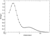 |
Fig. 1 Projected surface area distribution of MMS2 analog powder, with effective radius reff = 1.25 μm and effective variance νeff = 1.37. |
Compositional properties of the samples.
2.2 Surface roughness
Figure 2 shows the scanning electron microscope (SEM) images of the illuminated surface for each sample. The surfaces present a high degree of roughness at different scales that gradually increase from sample MASC-1 (Fig. 2a) to MASC-4 (Fig. 2d). The SEM images cover an area of 500×500 μm2.
To estimate surface roughness on smaller scales, atomic force microscopy (AFM) analysis was performed. We employed the tapping mode AFM of the Scientific Instrumentation Centre of the University of Granada. This technique images the sample topography by scanning its surface with an oscillating cantilever. It detects changes in tip-sample interaction forces by monitoring the amplitude of cantilever oscillation, thereby capturing the sample’s topography. In all cases, the scanning time was set to 10 minutes. For a fixed scanning time, regions with higher topographical complexity result in smaller scanned area. The results, summarized in Table 2, represent the (arithmetic) average height parameter Sa, measured in microns, with the corresponding scanned area (μm2) for three different patches analyzed for each sample. Sa is defined as the average absolute deviation of roughness irregularities from the mean line over a sampling length, as described by Gadelmawla et al. (2002). The scanned area varies due to the irregularities of the samples, as more complex topographies result in smaller scanned areas within the same time interval. Figure 3 provides examples of AFM images for each sample, where dark areas represent valleys and light regions indicate reliefs, as shown on the color scale bar. Each image covers an area of 20×20 μm2, except for MASC-2, which spans 30×30 μm2. Corresponding histograms display pixel counts over the absolute depth variations (in microns).
Based on the AFM analysis, MASC-1 is identified as the smoothest sample, exhibiting less dispersion in Sa values across the three selected patches. MASC-4 is the roughest, showing higher and more disperse Sa values. MASC-2 and MASC-3 exhibit similar Sa values, although MASC-2 displays a region with a larger scanned area (patch 2), indicating a smoother zone.
A visual analysis of the SEM images (Fig. 2) reveals that the surfaces exhibit structural features on larger scales compared to the previously measured surface roughness (Sa). The surfaces are marked by pits, ranging in size up to a few tens of micrometers. The number of these pits increases progressively from MASC-1, where no pits are observed, to MASC-4, which displays the highest number of cavities. The cavities possess complex structures with coves extending across multiple layers. These features can absorb a portion of the incident light and produce shadows that vary with the scattering angle.
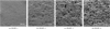 |
Fig. 2 SEM images of the MASC-1 (a), MASC-2 (b), MASC-3 (c), and MASC-4 (d) samples. The images cover an area of 500 × 500 μm2. |
Measured average height surface roughness parameter, Sa, and corresponding scanned area for the three patches analyzed for each sample by AFM analysis.
3 Experimental apparatus
The measurements were conducted at the IAA CODULAB, as described by Muñoz et al. (2020). This facility specializes in measuring the scattering matrices of various types of dust grains and can be configured for different experimental setups. These include measurements of clouds that consist of micron-sized particles (e.g., Frattin et al. 2019; Martín et al. 2021; Muñoz et al. 2021), and millimeter-sized pebbles (e.g., Muñoz et al. 2020; Frattin et al. 2022).
For this experiment, the setup was adapted to accommodate centimeter-sized cylindrical samples. Figure 4, panel a, shows a schematic overview of the adapted optical train as seen from above. We used a Coherent High Performance OBIST M diode laser emitting at 640 nm as light source. The laser light passes through a polarizer (P) and an electro-optic modulator (M). A beam expander is located after the modulator to widen the laser beam while maintaining a homogenous flux distribution. As shown in Fig. 4, panel c, the expanded beam illuminates a circular surface with a diameter of 0.3 cm on the base of the cylindrical sample. The sample is placed on a conical-tip flat black holder. To optimize the positioning of the surface of interest at the center of the ring, the holder is mounted on an x–y–z rotational stage (Fig. 4, panel b).
The scattered light is detected by a photomultiplier tube (PM detector) that moves along a 1 meter-diameter ring. A monitor (PM monitor) positioned at a fixed location on the ring, corrects for variations in intensity due to the different filters used to attenuate the incoming light beam when the signal saturates. Since the incoming light is absorbed within the sample and no radiation is transmitted, scattering occurs primarily near the surface, with negligible contributions from deeper within the sample. This observation aligns with the assumption of a semi-infinite medium. As a result, the measurable scattering angle, θ, is limited to the range of 90° to 177°. This range may be reduced in the case of rough surfaces, where light scattered parallel to the surface can be blocked by surface irregularities. In our case, the range in which the signal-to-noise ratio is acceptable is restricted to 94° to 177° (Fig. 4, panel a).
The combination of polarization modulation of the incident light and lock-in detection enables the measurement of all Fi,j elements of the 4×4 scattering matrix, F, for the sample. The matrix is described by the following relationship (Hovenier et al. 2004):
![Mathematical equation: $\[\left(\begin{array}{l}I_s \\Q_s \\U_s \\V_s\end{array}\right) \propto\left(\begin{array}{llll}F_{11} & F_{12} & F_{13} & F_{14} \\F_{21} & F_{22} & F_{23} & F_{24} \\F_{31} & F_{32} & F_{33} & F_{34} \\F_{41} & F_{42} & F_{43} & F_{44}\end{array}\right)\left(\begin{array}{l}I_0 \\Q_0 \\U_0 \\V_0\end{array}\right),\]$](/articles/aa/full_html/2025/05/aa53599-24/aa53599-24-eq1.png) (1)
(1)
where I0, Q0, U0, V0 and Is, Qs, Us, Vs are the Stokes vectors of the incident and scattered light beams, respectively. The elements Fij of the scattering matrix depend on the wavelength of the incoming light beam, the scattering angle θ and on the physical properties of the sample (size, morphology, and refractive index).
For an unpolarized incoming light beam, the element F11(θ) represents the scattered flux detected at angle θ and is referred to as the phase function. The ratio −F12(θ)/F11(θ) corresponds to the degree of linear polarization, also for an incident unpolarized light beam. These two quantities are particularly significant in astronomical applications, as they can be measured directly through both in situ and ground-based observations. In astronomical observations, the phase angle, α, is commonly used and is related to the scattering angle as α = 180°−θ. A comprehensive explanation of the scattering-matrix formalism is given by Hovenier et al. (2004) and van de Hulst (1957).
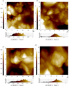 |
Fig. 3 AFM images of the MASC-1 (a), MASC-2 (b), MASC-3 (c), and MASC-4 (d) samples. The color bar at the left indicates the depth scale (in μm) in the color maps. The histogram at the bottom indicates the pixel counts over the absolute variation depth (in μm). |
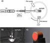 |
Fig. 4 Panel a: schematic overview of the adapted CODULAB optical train as seen from above. Shown is the filter wheel (FW), polarizer (P), modulator (M), diaphragm (D), analyzer (A), quarter wave plate (Q), and photomultiplier (PM). Panel b: the sample is located on a conical-tip holder mounted on an x–y–z rotating table. Panel c: illuminated cylindrical sample located on the conical holder. The illuminated area covers a circular region with a diameter of 0.3 cm. |
4 Results
The scattering matrix elements for the regolith-simulant samples were measured and are presented in Fig. 5. As mentioned in Sect. 3, the scattering angles of the measured data range from 94° to 177°, with measurements taken at 2° intervals between 94° and 150° and at 1° intervals between 150° and 177°. No light is received at angles smaller than 90°. The error bars represent the experimental uncertainties, and where no bar is visible, the error is smaller than the plotted symbol. As mentioned, the blocking effect of surface irregularities reduces the signal-to-noise ratio, resulting in significantly larger error bars for angles between 94° and 100° compared to the rest of angles.
The measured elements clearly reveal the impact of surface roughness. The curves for the various samples fall within relatively narrow ranges when plotted against the scattering angle, with MASC-1 (the smoothest) and MASC-4 (the roughest) defining the boundaries of these ranges. The measured F13(θ)/F11(θ), F14(θ)/F11(θ), F24(θ)/F11(θ), F31(θ)/F11(θ), and F41(θ)/F11(θ) are zero within the experimental errors in the full range of scattering angle. This suggests that the measured samples can be considered as media with mirror symmetry.
4.1 Phase function
The upper left panel of Fig. 5 displays the phase function curves of the samples on a logarithmic scale. To estimate the geometric albedo, the F11(θ) value of each sample was compared to that of a diffuse reflectance standard, a Spectralon (Labsphere SRT-99-020 AA-00823-000) with a nominal reflectance of 99%. Spectralon, a fluoropolymer with high diffuse reflectance, acts as a Lambertian surface, meaning its intensity follows the cosine law: I = I0cos(α), where α is the phase angle (α = 180° − θ). Radiance from a Lambertian surface remains constant across all scattering angles.
The samples albedo at 170° is calculated as ![Mathematical equation: $\[A\left(170^{\circ}\right)=F_{11}^{\mathrm{M}}\left(170^{\circ}\right) / F_{11}^{\mathrm{S}}\left(170^{\circ}\right)\]$](/articles/aa/full_html/2025/05/aa53599-24/aa53599-24-eq2.png) , where
, where ![Mathematical equation: $\[F_{11}^{\mathrm{M}}\left(170^{\circ}\right)\]$](/articles/aa/full_html/2025/05/aa53599-24/aa53599-24-eq3.png) and
and ![Mathematical equation: $\[F_{11}^{\mathrm{S}}\left(170^{\circ}\right)\]$](/articles/aa/full_html/2025/05/aa53599-24/aa53599-24-eq4.png) are the phase function values at 170° for the sample and the Spectralon, respectively. The results, expressed as percentages (%), are listed in Table 3. Due to instrumental limitations, it is not possible to observe the geometric albedo at a scattering angle of 180 degrees, that is, opposition. From this point forward, the term 170°-albedo refers to the measurements taken at 170 degrees, used as a proxy for the geometric albedo. All F11(θ) curves displayed in Fig. 5 are normalized to their corresponding albedo at 170°. Among the samples, MASC-1 is the brightest, with a 170°-albedo of 40%, followed by MASC-2 and MASC-3, which have lower albedos. MASC-4 is the darkest, with an albedo of 27%. This indicates an inverse relationship between albedo and surface roughness (Sa): higher surface roughness correlates with lower albedo.
are the phase function values at 170° for the sample and the Spectralon, respectively. The results, expressed as percentages (%), are listed in Table 3. Due to instrumental limitations, it is not possible to observe the geometric albedo at a scattering angle of 180 degrees, that is, opposition. From this point forward, the term 170°-albedo refers to the measurements taken at 170 degrees, used as a proxy for the geometric albedo. All F11(θ) curves displayed in Fig. 5 are normalized to their corresponding albedo at 170°. Among the samples, MASC-1 is the brightest, with a 170°-albedo of 40%, followed by MASC-2 and MASC-3, which have lower albedos. MASC-4 is the darkest, with an albedo of 27%. This indicates an inverse relationship between albedo and surface roughness (Sa): higher surface roughness correlates with lower albedo.
Direct measurements of the Martian-regolith simulant geometric albedo at 180° in the R band (700 nm) yield a value of 0.289±0.003 (Mallama 2007). This is consistent with the result obtained for the roughest sample measured in this work, MASC-4.
Figure 6 shows the phase functions for Spectralon and the samples on a linear scale. The measured F11(θ) for Spectralon is normalized to 1 at 170°, so that the value of each curve at 170° corresponds to the 170° albedo.
One interpretation of these results relates to the shape of the roughness. Surface topography is crucial for interpreting the photometry of regolith-like surfaces and the shape of the roughness influences their scattering behavior (Shkuratov et al. 2005). Thus, we needed to take into account both the surface roughness in terms of vertical depth, Sa, and the shape of the asperities rising on a larger scale. The surfaces of these samples show cavities with peculiar shapes larger than the wavelength and with slope angles greater than 90°, able to absorb the incoming light and create shadows that change depending on the scattering angle. Thus, one possible explanation is that absorption and shadowing effects dominate when large-scale topography with photon-trapping cavities are present, reducing light and darkening the sample.
4.2 Degree of linear polarization
The upper-middle panel of Fig. 5 shows the degree of linear polarization curves, −F12(θ)/F11(θ). From opposition at θ = 180°, these curves generally increase with decreasing scattering angle and exhibit a shallow NPB. Figure 7 provides a closer look at the degree of linear polarization for the four samples between 120° and 177°. While the values are somewhat scattered, a slight trend emerges: MASC-1 shows a higher, more linear curve, whereas MASC-4 exhibits a flatter, more dispersed pattern.
The NPB is a well-known feature observed in measurements of atmosphere-less bodies covered with regolith (e.g., Rosenbush et al. 2015; Cellino et al. 2015) and in cometary comae (Kiselev et al. 2015). At small phase angles, the polarization plane coincides with the scattering plane, resulting in negative polarization values. The shape, depth, and position of the inversion angle of the NPB depend on several surface properties, including roughness, topography, monomers size, packing density, and composition.
The primary mechanisms responsible for the NPB are single-particle scattering and CB (Muinonen et al. 2015, and references therein). The proportions of single and multiple scattering due to the particles forming the surface contribute to the formation of NPB, particularly in densely packed media (e.g., Shkuratov et al. 2004, 2006).
Our results reveal a shallow NPB within the scattering angle range of 160°–177° for all samples. Although the data are somewhat scattered, making it difficult to pinpoint a precise inversion angle, a trend emerges. MASC-1 exhibits a higher degree of linear polarization with the NPB shifted to larger scattering angles, whereas MASC-4 shows a flatter degree of linear polarization with the NPB appearing at smaller scattering angles (see Fig. 7).
Multiple scattering is more pronounced in low-absorbing materials, that is, materials with higher albedo (Li et al. 2015; Shkuratov et al. 2006) and such materials tend to display shallower NPBs compared to high-absorbing ones. Intriguingly, our samples are in direct conflict with the generally accepted trend: more prominent NPBs are here measured for samples with higher albedos. The present NPB trend can be explained by the interplay of total, single, and multiple scattering. With increasing roughness, the proportion of single scattering decreases, resulting in weakening NPB from single particles. In the phase angles of the present measurements, this weakening trend is not counterbalanced by the increasing relative significance of NPB from CB. One may predict that, closer to zero phase angle, the NPB from CB would start to predominate (Muinonen et al. 2025).
To further investigate the behavior of the NPB, we compared it to the curve generated by a cloud of dust composed of the same material. Figure 8 shows the degree of linear polarization for the smoothest sample (MASC-1), the roughest sample (MASC-4), and for a dust cloud consisting of the MMS2 powder. In particular, we show the measured data for the MMS2-M sample as described by Martikainen et al. (2024). The MMS2-M sample shares the same composition as the dust used in the regolith-simulant samples but features a size distribution with an effective radius reff = 2.3 μm and an effective variance νeff = 0.28 (slightly narrower than the distribution used for the MASC samples). The NPBs observed in particulate media are shallower and have inversion angles shifted to larger scattering angles compared to those produced by the cloud of dust particles. This behavior is in agreement with the explanation above based on the interplay of single and multiple scattering.
Comparative laboratory works of Shkuratov et al. (2002, 2004, 2006, 2007) and Hadamcik et al. (2011) regarding particulate surfaces and particle clouds demonstrated the same behavior: particulate surfaces produce shallower NPBs compared to particle clouds. They also observed that smooth surfaces exhibit deeper NPBs compared to rough surfaces with reliefs, further highlighting the significant role of surface topography in influencing the degree of linear polarization.
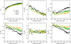 |
Fig. 5 Measured scattering matrix elements as a function of the scattering angle for MASC-1 (black dots), MASC-2 (gray triangles), MASC-3 (green stars), and MASC-4 (orange squares). The F11 curves are normalized to their corresponding albedo at 170 degrees (see Table 3). |
Albedo (A) at a 170° scattering angle in percent.
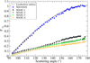 |
Fig. 6 Phase function F11(θ) for the regolith-simulant samples, the Spectralon (blue diamonds), and the Lambertian surface (black line) in linear scale. The values for the Spectralon are normalized to 1 at 170°, so the value of the samples at 170° corresponds to their albedo. |
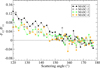 |
Fig. 7 Degree of linear polarization curves −F12(θ)/F11(θ) of the four samples in the scattering angle range 120°–177°. |
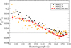 |
Fig. 8 Degree of linear polarization curves of samples MASC-1 (black) and MASC-4 (orange) together with dust sample MMS2-M (red) from Martikainen et al. (2024). |
4.3 Diagonal elements of the scattering matrix
The trends in the scattering matrix elements F22(θ)/F11(θ) (upper right panel of Fig. 5), F33(θ)/F11(θ) (lower left), and F44(θ)/F11(θ) (lower right) are particularly noticeable. The smoother the sample surface, the steeper these curves appear. For instance, MASC-1, with the lowest roughness, shows the steepest curves. As surface roughness increases, the curves flatten, with MASC-4 (the roughest) exhibiting the flattest behavior. MASC-2 and MASC-3 display similar trends, consistent with their comparable surface properties. These trends are consistent with the geometric optics simulations by Väisänen et al. (2020b), and as such the interplay of total, single, and multiple scattering explains the trends. Increasing roughness decreases both the total scattering and the proportion of single to multiple scattering. The latter trend follows from the interactions near the surface being replaced by the more complex interactions deeper in the volume. The net effect is increasing depolarization with increasing roughness, shown by the measured matrix element ratios F22(θ)/F11(θ), F33(θ)/F11(θ), and F44(θ)/F11(θ).
5 Discussion
In the present study, the samples that effectively represent planetary regolith exhibit highly heterogeneous structures with roughness on multiple scales and complex topography. These features dominate their scattering behavior.
For surfaces, the conditions for single scattering are no longer applicable. Single scattering generally applies to optically thin media, such as atmospheric aerosols, interplanetary dust, or interstellar dust, where each particle is excited solely by the external incident field. In contrast, planetary regolith, with its high particle concentration, forms an optically thick medium where multiple scattering must be considered. It implies excitation of the particle by the incident field as well as by the scattered field from all the surrounding particles. Detailed reviews of observations and theoretical interpretations of multiple scattering effects can be found in works, for instance, by Muinonen et al. (2015), Rosenbush et al. (2015), Mishchenko et al. (2007), Mackowski & Mishchenko (1996), and Shkuratov et al. (1994).
The primary physical mechanisms influencing the scattering behavior of particulate media include incoherent single and multiple scattering, with a due account for shadowing and CB. These mechanisms depend on the physical properties of the medium, such as its composition, roughness, and volume density, and by extension its albedo.
One key finding from this study is the inverse relationship between surface roughness and albedo: as surface roughness increases, albedo decreases. Roughness was measured on both small scales using AFM analysis (vertical depth of 2 microns) and larger scales through visual examination of the SEM images (tens of microns). The larger-scale structures, with their complex shapes and porous features, can trap and absorb light. In these cases, the shape of the structures becomes the dominant parameter, with absorption and shadowing emerging as primary mechanisms.
Shadowing occurs when surface structures physically block certain light paths, preventing the light from reaching the observer or being scattered by other parts of the surface. This effect is particularly pronounced in rough or densely packed particulate media, where geometric optics dominate on scales larger than the wavelength. Shadowing reduces the amount of scattered light in certain directions and creates dark areas in the scattered light pattern.
The inverse relation between albedo (reflectance) and surface roughness observed in this study is in agreement with laboratory measurements on particulate surfaces (Shepard & Helfenstein 2011; Capaccioni et al. 1990), geological research involving field measurements of snow albedo, (Larue et al. 2020; Lhermitte et al. 2014), and studies in computer graphics (Sun 2023). Furthermore, since composition, volume density, and roughness influence the behavior of the phase function, photometric models of regolith surfaces must incorporate these properties to accurately derive albedo from reflectance measurements (Hapke et al. 1993; Mishchenko et al. 1999; Hasselmann et al. 2021, 2024; Björn et al. 2024).
Many studies focus on the phase function F11(θ) and the degree of linear polarization −F12(θ)/F11(θ) as these elements can be directly measured through ground-based and in situ observations of Solar System bodies (Rosenbush et al. 2015; Cellino et al. 2015; Belskaya & Bagnulo 2015). Polarimetric observations of these bodies are especially valuable near opposition at small phase angles, where astronomical observations are more numerous, and the surface microstructures have a significant impact on the light-scattering process. Our present results indicate a complex relationship between the albedo, degree of linear polarization, and surface roughness. This is in violation with the so-called Umov’s law for the albedo-polarization relationship that would suggest more pronounced polarization for lower albedo.
Considerable attention has been given to the backscattering region and its characteristic features, such as the NPB and the BOE. The former is generally attributed to the CB and single-particle mechanisms (Muinonen et al. 2025; Muinonen et al. 2012; Rosenbush et al. 2015; Mishchenko et al. 2010). Coherent backscattering refers to the situation where the interference of waves scattered along reciprocal paths has a significant impact on the light-scattering signal. In the backscattering region, this occurs when rays are scattered by the same particles, but in opposite directions, and interfere constructively (e.g., Muinonen 1990; Hapke 1990; Shkuratov 1989). In the exact backscattering direction, the scattered waves traverse identical path lengths and the interference is constructive. In other directions, the interference can be constructive or destructive, depending on the specific path lengths of the interfering waves. In the present work, the samples show shallow NPBs, suggesting a significant contribution from single scattering neutralized by multiple scattering, which is promoted by surface roughness and the shape of the asperities.
Laboratory experiments on particulate surfaces show that introducing surface reliefs reduces backscattering effects due to decreased proportion of single scattering, leading to shallower NPBs and BOEs (Shkuratov et al. 2002, 2004, 2006, 2007; Renard et al. 2010; Hadamcik et al. 2011; Geake & Geake 1990). Conversely, surfaces with fine structures at the wavelength scale produce more pronounced NPBs (Shkuratov et al. 2002). Laboratory measurements of forsterite micrometric powder (Muñoz et al. 2021) and of the same Martian analog material used in this work, but in the form of particle clouds (Martikainen et al. 2023), indicate that the NPB diminishes as particle size increases relative to the wavelength.
Theoretical and numerical studies of surfaces with multiple-scale roughness and high packing densities are essential for understanding the mechanisms that govern their scattering behavior. This study underscores the importance of considering surface roughness shapes when developing realistic models. The samples analyzed in this work contain a dust volume percentage exceeding 40% (as in the case of MASC-4), resulting in a very high packing density.
Simulations with irregularly shaped particles and high packing density have been conducted by Väisänen et al. (2020b), who modeled discrete random media using a hybrid RT and geometric optics approach. They divided the medium into a mantle of Gaussian-random-sphere particles (Muinonen et al. 1996) and a diffusely scattering core. Their results, with packing densities up to 40%, are consistent with those of the present study, showing a very shallow NPB and F22(θ)/F11(θ) elements resembling the shape of the measured F22(θ)/F11(θ) curves obtained for the cylinder aggregates. They also found that high packing densities suppress the brightness increase in the backscattering direction.
Grynko et al. (2020) also studied high-packing-density surfaces, emphasizing the importance of using irregularly shaped particles to simulate particulate media in the backscattering regime. Furthermore, Grynko et al. (2022) demonstrated that backscattering polarization can be explained for surfaces with a low geometric albedo of a few percent through first-order and second-order scattering in the upper layer of a particulate structure with a packing density of 50%.
6 Conclusions
We measured the scattering matrix of four Martian analog samples with varying surface roughnesses. These represent the first surface measurements conducted at CODULAB, and the experimental apparatus was specifically adapted to meet the new requirements. Our results reveal a clear trend in the scattering matrix elements, which is strongly influenced by the complex surface topography of the samples. We identified an inverse relationship between the surface roughness and albedo: as the surface roughness increases, the albedo decreases. This effect likely arises from absorption and shadowing. Larger pores within the geometric optics regime form cavities that absorb radiation and cast shadows, reducing the amount of scattered light that reaches the detector. Additionally, we observed a very shallow NPB, which is likely diminished by the increased proportion of multiple scattering.
This study highlights the crucial role of topography and the shape of the large-scale structures of regolith in determining the scattering behavior of dense surfaces. Further investigations into densely packed media, taking the heterogeneous structures of surfaces and the irregular shapes of particles into account, would be invaluable for interpreting astronomical data.
This work is part of an ongoing project; we plan to extend our measurements to the blue wavelength domain to study the effects of absorption on rough surfaces. Additionally, we aim to measure the scattering matrices of aggregates derived from portions of the regolith-simulant samples. These results will provide essential insights into the impact of surface roughness on the regolith of atmosphere-less bodies, such as asteroids, and the scattering properties of cometary comae.
Data availability
The experimental data are freely available at the Granada-Amsterdam light scattering database, scattering.iaa.es, upon request via citation of this paper and Muñoz et al. (2025).
Acknowledgements
The authors sincerely thank Antoine Pommerol for his valuable feedback which helped us to improve a previous version of this manuscript. Authors acknowledge support by grant PID2021-123370OB-100/AEI/10.13039/501100011033/FEDER funded by MCIN/AEI/10.13039/501100011033 and Severo Ochoa grant CEX2021-001131-S funded by MCIN/AEI/10.13039/501100011033. This project also was supported by the NASA KPLO Participating Scientist Program NNH18ZDA001N-KPLOPSP, grant 80NSSC21K0755. Research by KM and AP supported by the Research Council of Finland grants Nos. 336546, 345115, and 359893. We thank Rocío Márquez Crespo and Fátima Linares Ordóñez from the Scientific InstrumentationCentre of the University of Granada for providing the SEM and AFM images, respectively.
References
- Belskaya, I., & Bagnulo, S. 2015, Transneptunian Objects and Centaurs, eds. L. Kolokolova, J. Hough, & A.-C. Levasseur-Regourd (Cambridge University Press), 405 [Google Scholar]
- Björn, V., Muinonen, K., Penttilä, A., & Domingue, D. 2024, PSJ, 5, 260 [Google Scholar]
- Capaccioni, F., Cerroni, P., Barucci, M. A., & Fulchignoni, M. 1990, Icarus, 83, 325 [Google Scholar]
- Cellino, A., Gil-Hutton, R., & Belskaya, I. 2015, Asteroids, eds. L. Kolokolova, J. Hough, & A.-C. Levasseur-Regourd (Cambridge University Press), 360 [Google Scholar]
- Frattin, E., Muñoz, O., Moreno, F., et al. 2019, MNRAS, 484, 2198 [Google Scholar]
- Frattin, E., Martikainen, J., Muñoz, O., et al. 2022, MNRAS, 517, 5463 [NASA ADS] [CrossRef] [Google Scholar]
- Gadelmawla, E., Koura, M., Maksoud, T., Elewa, I., & Soliman, H. 2002, J. Mater. Process. Technol., 123, 133 [CrossRef] [Google Scholar]
- Geake, J. E., & Geake, M. 1990, MNRAS, 245, 46 [NASA ADS] [Google Scholar]
- Grynko, Y., Shkuratov, Y., & Förstner, J. 2020, J. Quant. Spec. Radiat. Transf., 255, 107234 [Google Scholar]
- Grynko, Y., Shkuratov, Y., Alhaddad, S., & Förstner, J. 2022, Icarus, 384, 115099 [NASA ADS] [CrossRef] [Google Scholar]
- Hadamcik, E., Renard, J.-B., Levasseur-Regourd, A. C., & Lasue, J. 2011, in Polarimetric Detection, Characterization and Remote Sensing, eds. M. I. Mishchenko, Y. S. Yatskiv, V. K. Rosenbush, & G. Videen (Dordrecht: Springer Netherlands), 137 [CrossRef] [Google Scholar]
- Hansen, J. E., & Travis, L. D. 1974, Space Sci. Rev., 16, 527 [Google Scholar]
- Hapke, B. 1990, Icarus, 88, 407 [NASA ADS] [CrossRef] [Google Scholar]
- Hapke, B. W., Nelson, R. M., & Smythe, W. D. 1993, Science, 260, 509 [CrossRef] [Google Scholar]
- Hasselmann, P. H., Fornasier, S., Barucci, M. A., et al. 2021, Icarus, 357, 114106 [Google Scholar]
- Hasselmann, P. H., Della Corte, V., Pravec, P., et al. 2024, PSJ, 5, 91 [Google Scholar]
- Hovenier, J. W., Van Der Mee, C., & Domke, H. 2004, Transfer of Polarized Light in Planetary Atmospheres: Basic Concepts and Practical Methods, 318 [Google Scholar]
- Jeong, M., Kim, S. S., Garrick-Bethell, I., et al. 2015, ApJS, 221, 16 [Google Scholar]
- Jeong, M., Choi, Y.-J., Kang, K.-I., et al. 2023, J. Korean Astron. Soc., 56, 293 [Google Scholar]
- Kiselev, N., Rosenbush, V., Levasseur-Regourd, A.-C., & Kolokolova, L. 2015, Comets, eds. L. Kolokolova, J. Hough, & A.-C. Levasseur-Regourd (Cambridge University Press), 379 [Google Scholar]
- Larue, F., Picard, G., Arnaud, L., et al. 2020, Cryosphere, 14, 1651 [Google Scholar]
- Lhermitte, S., Abermann, J., & Kinnard, C. 2014, Cryosphere, 8, 1069 [Google Scholar]
- Li, J. Y., Helfenstein, P., Buratti, B., Takir, D., & Clark, B. E. 2015, in Asteroids IV, eds. P. Michel, F. E. DeMeo, & W. F. Bottke, 129 [Google Scholar]
- Mackowski, D. W., & Mishchenko, M. I. 1996, J. Opt. Soc. Am., 13, 2266 [NASA ADS] [CrossRef] [Google Scholar]
- Mallama, A. 2007, Icarus, 192, 404 [NASA ADS] [CrossRef] [Google Scholar]
- Markkanen, J., & Penttilä, A. 2023, J. Quant. Spec. Radiat. Transf., 310, 108733 [Google Scholar]
- Martikainen, J., Muñoz, O., Jardiel, T., et al. 2023, ApJS, 268, 47 [Google Scholar]
- Martikainen, J., Muñoz, O., Gómez Martín, J. C., et al. 2024, ApJS, 273, 28 [Google Scholar]
- Martín, J. C. G., Guirado, D., Frattin, E., et al. 2021, J. Quant. Spec. Radiat. Transf., 271, 107761 [Google Scholar]
- Mishchenko, M. I., Dlugach, Z. M., Yanovitskij, E. G., & Zakharova, N. T. 1999, J. Quant. Spec. Radiat. Transf., 63, 409 [Google Scholar]
- Mishchenko, M. I., Liu, L., Mackowski, D. W., Cairns, B., & Videen, G. 2007, Opt. Express, 15, 2822 [Google Scholar]
- Mishchenko, M. I., Rosenbush, V. K., Kiselev, N. N., et al. 2010, arXiv e-prints [arXiv:1010.1171] [Google Scholar]
- Muñoz, O., Moreno, F., Guirado, D., et al. 2011, Icarus, 211, 894 [Google Scholar]
- Muinonen, K. O. 1990, PhD thesis, University of Helsinki, Finland [Google Scholar]
- Muinonen, K., Nousiainen, T., Fast, P., Lumme, K., & Peltoneimi, J. 1996, J. Quant. Spec. Radiat. Transf., 55, 577 [Google Scholar]
- Muinonen, K., Parviainen, H., Näränen, J., et al. 2011, A&A, 531, A150 [NASA ADS] [CrossRef] [EDP Sciences] [Google Scholar]
- Muinonen, K., Mishchenko, M. I., Dlugach, J. M., et al. 2012, ApJ, 760, 118 [Google Scholar]
- Muinonen, K., Penttilä, A., & Videen, G. 2015, in Polarimetry of Stars and Planetary Systems, eds. L. Kolokolova, J. Hough, & A.-C. Levasseur-Regourd, 114 [CrossRef] [Google Scholar]
- Muinonen, K., Leppälä, A., & Markkanen, J. 2025, J. Quant. Spec. Radiat. Transf., 330, 109226 [Google Scholar]
- Muñoz, O., Moreno, F., Gómez-Martín, J. C., et al. 2020, ApJS, 247, 19 [CrossRef] [Google Scholar]
- Muñoz, O., Frattin, E., Jardiel, T., et al. 2021, ApJS, 256, 17 [CrossRef] [Google Scholar]
- Muñoz, O., Frattin, E., Martikainen, J., et al. 2025, J. Quant. Spec. Radiat. Transf., 331, 109252 [Google Scholar]
- Nelson, R. M., Boryta, M. D., Hapke, B. W., et al. 2018, Icarus, 302, 483 [NASA ADS] [CrossRef] [Google Scholar]
- Ovcharenko, A. A., Bondarenko, S. Y., Zubko, E. S., et al. 2006, J. Quant. Spec. Radiat. Transf., 101, 394 [Google Scholar]
- Penttilä, A., Markkanen, J., Väisänen, T., et al. 2021, J. Quant. Spec. Radiat. Transf., 262, 107524 [Google Scholar]
- Peters, G. H., Abbey, W., Bearman, G. H., et al. 2008, Icarus, 197, 470 [Google Scholar]
- Poch, O., Cerubini, R., Pommerol, A., Jost, B., & Thomas, N. 2018, J. Geophys. Res., 123, 2564 [Google Scholar]
- Renard, J.-B., Francis, M., Hadamcik, E., et al. 2010, Appl. Opt., 49, 3552 [Google Scholar]
- Rosenbush, V., Kiselev, N., & Afanasiev, V. 2015, in Polarimetry of Stars and Planetary Systems, eds. L. Kolokolova, J. Hough, & A.-C. Levasseur-Regourd, 340 [CrossRef] [Google Scholar]
- Shepard, M. K., & Helfenstein, P. 2011, Icarus, 215, 526 [Google Scholar]
- Shkuratov, Y. G. 1989, Sol. Syst. Res., 23, 111 [Google Scholar]
- Shkuratov, Y. G., Muinonen, K., Bowell, E., et al. 1994, Earth Moon Planets, 65, 201 [NASA ADS] [CrossRef] [Google Scholar]
- Shkuratov, Y., Ovcharenko, A., Zubko, E., et al. 2002, Icarus, 159, 396 [CrossRef] [Google Scholar]
- Shkuratov, Y., Ovcharenko, A., Zubko, E., et al. 2004, J. Quant. Spec. Radiat. Transf., 88, 267 [NASA ADS] [CrossRef] [Google Scholar]
- Shkuratov, Y. G., Stankevich, D. G., Petrov, D. V., et al. 2005, Icarus, 173, 3 [Google Scholar]
- Shkuratov, Y., Bondarenko, S., Ovcharenko, A., et al. 2006, J. Quant. Spec. Radiat. Transf., 100, 340 [CrossRef] [Google Scholar]
- Shkuratov, Y., Bondarenko, S., Kaydash, V., et al. 2007, J. Quant. Spec. Radiat. Transf., 106, 487 [Google Scholar]
- Shkuratov, Y., Opanasenko, N., Zubko, E., et al. 2007, Icarus, 187, 406 [NASA ADS] [CrossRef] [Google Scholar]
- Shkuratov, Y., Videen, G., & Kaydash, V. 2025, Optics of the Moon (Elsevier) [Google Scholar]
- Spadaccia, S., Patty, C. H. L., Capelo, H. L., Thomas, N., & Pommerol, A. 2022, A&A, 665, A49 [NASA ADS] [CrossRef] [EDP Sciences] [Google Scholar]
- Spadaccia, S., Patty, C. H. L., Thomas, N., & Pommerol, A. 2023, Icarus, 396, 115503 [NASA ADS] [CrossRef] [Google Scholar]
- Stankevich, D., Shkuratov, Y., Sim, C. K., et al. 2023, J. Quant. Spec. Radiat. Transf., 296, 108457 [Google Scholar]
- Stankevich, D. G., Shkuratov, Y. G., & Muinonen, K. 1999, J. Quant. Spec. Radiat. Transf., 63, 445 [Google Scholar]
- Sun, L. 2023, Heliyon, 9, e15928 [Google Scholar]
- Väisänen, T., Markkanen, J., Hadamcik, E., et al. 2020a, Opt. Lett., 45, 1679 [Google Scholar]
- Väisänen, T., Martikainen, J., & Muinonen, K. 2020b, J. Quant. Spec. Radiat. Transf., 241, 106719 [Google Scholar]
- van de Hulst, H. C. 1957, Light Scattering by Small Particles (New York: John Wiley & Sons) [Google Scholar]
- Waza, A., Kjer, J., Peiteado, M., et al. 2023, Planet. Space Sci., 227, 105638 [Google Scholar]
All Tables
Measured average height surface roughness parameter, Sa, and corresponding scanned area for the three patches analyzed for each sample by AFM analysis.
All Figures
|
Fig. 1 Projected surface area distribution of MMS2 analog powder, with effective radius reff = 1.25 μm and effective variance νeff = 1.37. |
| In the text | |
|
Fig. 2 SEM images of the MASC-1 (a), MASC-2 (b), MASC-3 (c), and MASC-4 (d) samples. The images cover an area of 500 × 500 μm2. |
| In the text | |
|
Fig. 3 AFM images of the MASC-1 (a), MASC-2 (b), MASC-3 (c), and MASC-4 (d) samples. The color bar at the left indicates the depth scale (in μm) in the color maps. The histogram at the bottom indicates the pixel counts over the absolute variation depth (in μm). |
| In the text | |
|
Fig. 4 Panel a: schematic overview of the adapted CODULAB optical train as seen from above. Shown is the filter wheel (FW), polarizer (P), modulator (M), diaphragm (D), analyzer (A), quarter wave plate (Q), and photomultiplier (PM). Panel b: the sample is located on a conical-tip holder mounted on an x–y–z rotating table. Panel c: illuminated cylindrical sample located on the conical holder. The illuminated area covers a circular region with a diameter of 0.3 cm. |
| In the text | |
|
Fig. 5 Measured scattering matrix elements as a function of the scattering angle for MASC-1 (black dots), MASC-2 (gray triangles), MASC-3 (green stars), and MASC-4 (orange squares). The F11 curves are normalized to their corresponding albedo at 170 degrees (see Table 3). |
| In the text | |
|
Fig. 6 Phase function F11(θ) for the regolith-simulant samples, the Spectralon (blue diamonds), and the Lambertian surface (black line) in linear scale. The values for the Spectralon are normalized to 1 at 170°, so the value of the samples at 170° corresponds to their albedo. |
| In the text | |
|
Fig. 7 Degree of linear polarization curves −F12(θ)/F11(θ) of the four samples in the scattering angle range 120°–177°. |
| In the text | |
|
Fig. 8 Degree of linear polarization curves of samples MASC-1 (black) and MASC-4 (orange) together with dust sample MMS2-M (red) from Martikainen et al. (2024). |
| In the text | |
Current usage metrics show cumulative count of Article Views (full-text article views including HTML views, PDF and ePub downloads, according to the available data) and Abstracts Views on Vision4Press platform.
Data correspond to usage on the plateform after 2015. The current usage metrics is available 48-96 hours after online publication and is updated daily on week days.
Initial download of the metrics may take a while.