Fig. 3
Download original image
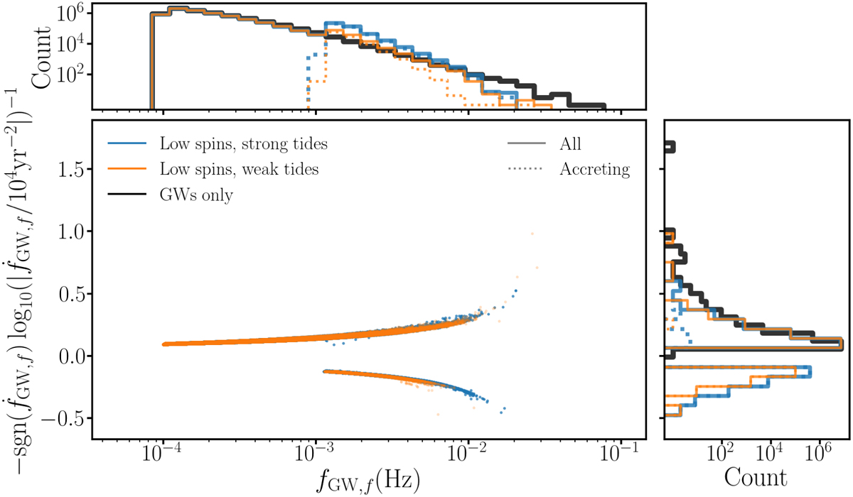
Comparison of the populations in the ![]() plane for the ‘low spins, strong tides’ (in blue) and ‘low spins, weak tides’ (in orange) scenarios, where
plane for the ‘low spins, strong tides’ (in blue) and ‘low spins, weak tides’ (in orange) scenarios, where ![]() . This quantity has the same sign and monotonic behaviour as
. This quantity has the same sign and monotonic behaviour as ![]() . The black lines in the upper and right panels show the result in the ‘GWs only’ scenario. Accreting systems are typically those with
. The black lines in the upper and right panels show the result in the ‘GWs only’ scenario. Accreting systems are typically those with ![]() < 0. We recall that we keep only DWDs that have fGW,f ≥ 0.1 mHz in the ‘GWs only’ case, which explains why the distribution goes to 0 below this limit and for small positive values of
< 0. We recall that we keep only DWDs that have fGW,f ≥ 0.1 mHz in the ‘GWs only’ case, which explains why the distribution goes to 0 below this limit and for small positive values of ![]() .
.
Current usage metrics show cumulative count of Article Views (full-text article views including HTML views, PDF and ePub downloads, according to the available data) and Abstracts Views on Vision4Press platform.
Data correspond to usage on the plateform after 2015. The current usage metrics is available 48-96 hours after online publication and is updated daily on week days.
Initial download of the metrics may take a while.