| Issue |
A&A
Volume 691, November 2024
|
|
|---|---|---|
| Article Number | A272 | |
| Number of page(s) | 7 | |
| Section | Stellar atmospheres | |
| DOI | https://doi.org/10.1051/0004-6361/202451417 | |
| Published online | 15 November 2024 | |
Magnetic field of the roAp star KIC 10685175: Observations versus theory
1
Department of Astronomy, Peking University,
Beijing
100871,
China
2
The Kavli Institute for Astronomy and Astrophysics, Peking University,
Beijing
100871,
China
3
Leibniz-Institut für Astrophysik Potsdam (AIP),
An der Sternwarte 16,
14482
Potsdam,
Germany
4
School of Physics and Astronomy, Beijing Normal University,
Beijing
100875,
China
5
Institute for Frontiers in Astronomy and Astrophysics, Beijing Normal University,
Beijing
102206,
China
6
Centre for Space Research, North-West University,
Mahikeng
2745,
South Africa
7
Jeremiah Horrocks Institute, University of Central Lancashire,
Preston
PR1 2HE,
UK
★ Corresponding authors; This email address is being protected from spambots. You need JavaScript enabled to view it.
; This email address is being protected from spambots. You need JavaScript enabled to view it.
Received:
8
July
2024
Accepted:
28
September
2024
Abstract
Context. KIC 10685175 is a roAp star whose polar magnetic field is predicted to be 6 kG through a nonadiabatic axisymmetric pulsation theoretical model.
Aims. In this work, we aim to measure the magnetic field strength of KIC 10685175 using high-resolution spectropolarimetric observations, and compare it with the one predicted by the theoretical model.
Methods. Two high-resolution unpolarized spectra have been analyzed to ascertain the presence of magnetically split lines and derive the iron abundance of this star through equivalent width measurements of 10 Fe lines. One polarized spectrum has been used to measure the mean longitudinal magnetic field with the least-squares deconvolution technique. Further, to examine the presence of chemical spots on the stellar surface, we have measured the mean longitudinal magnetic fields using different lines belonging to different elements.
Results. From the study of two high-resolution unpolarized spectra, we obtained the spectroscopic atmospheric parameters including the effective temperature (Teff), surface gravity (log 𝑔), iron abundance ([Fe/H]), abundance ratio of alpha elements to iron ([α/Fe]), and micro-turbulent velocity (Vmic). The final result is [Teff, log g, [Fe/H], [α/Fe], Vmic)]=[8250 ± 200 K, 4.4 ± 0.1, −0.4 ± 0.2, 0.16 ± 0.1, 1.73 ± 0.2 km s−1]. Although the Fe absorption lines appear relatively weak in comparison to typical Ap stars with similar Teff, the lines belonging to rare earth elements (Eu and Nd) are stronger than those in chemically normal stars, indicating the peculiar nature of KIC 10685175. The mean longitudinal magnetic field, 〈Bℓ〉 = −226 ± 39 G, was measured in the polarized spectrum, but magnetically split lines were not detected. No significant line profile variability is evident in our spectra. Also, the longitudinal magnetic field strengths measured using line masks constructed for different elements are rather similar. Due to the poor rotation phase coverage of our data, additional spectroscopic and polarimetric observations are needed to allow us to come to any conclusions about the inhomogeneous element distribution over the stellar surface.
Conclusions. The estimated polar magnetic field is 4.8 ± 0.8 kG, which is consistent with the predicted polar magnetic field strength of about 6kG within 3σ. This work therefore provides support for the pulsation theoretical model.
Key words: stars: abundances / stars: chemically peculiar / stars: magnetic field / stars: individual: KIC 10685175
© The Authors 2024
 Open Access article, published by EDP Sciences, under the terms of the Creative Commons Attribution License (https://creativecommons.org/licenses/by/4.0), which permits unrestricted use, distribution, and reproduction in any medium, provided the original work is properly cited.
This article is published in open access under the Subscribe to Open model. This email address is being protected from spambots. You need JavaScript enabled to view it. to support open access publication.
1 Introduction
Ap stars are chemically peculiar stars of spectral type A that have overabundances of iron-peak and rare-earth elements, such as Si, Cr, Sr, and Eu (Preston 1974). A prime factor governing the peculiarities of Ap stars is the strong magnetic fields they host. These magnetic fields are roughly dipolar, with typical field strengths of a kilo Gauss, or more. The strong magnetic field suppresses convection, providing a stable environment for ions with many absorption features to be lifted by radiation pressure against gravity and kept stratified in the observable surface layers. At the same time, some other elements, especially helium, which have few absorption lines near flux maximum in the outer envelope of the star, settle down, affected by gravity. The element stratification in the presence of a magnetic field causes the peculiarities of surface abundance.
Some Ap stars exhibit high-overtone, low-degree pressure pulsation modes. These are called rapidly oscillating Ap (roAp) stars and they have many pulsation features. In the HR diagram, these stars overlap with δ Sct stars, which are nonmagnetic (or extremely weakly magnetic). Generally, the δ Sct stars pulsate in low-radial-overtone p modes, while the roAp stars pulsate in high-radial-overtone magneto-acoustic modes. Also, unlike the nonmagnetic stars, the pulsation axes of roAp stars are almost symmetric about the oblique quasi-dipolar magnetic field (Kochukhov 2003; Saio 2005; Bigot & Kurtz 2011). Thus, it is believed that the strong magnetic fields of roAp stars play an essential role in the pulsation mode excitation and selection (Balmforth et al. 2001; Saio 2005; Cunha 2006).
The pulsation axes of roAp stars are affected by the presence of a magnetic field, as is discussed in Dziembowski & Goode (1996), Cunha & Gough (2000), and Saio & Gautschy (2004), which means the pulsation mode is not a pure dipole or quadrupole (or higher). Saio (2005) provides a method to model the quadrupole or dipole pulsation distorted by dipole magnetic fields. In this model, the polar magnetic field is predicted by comparing the theoretical pulsation data with the observed one. Further, this model is used to estimate the polar magnetic field strength, effective temperature, mass, and other stellar parameters (Holdsworth et al. 2016, 2018). On the other hand, testing the consistency between the field measurements and the predictions on the magnetic field strengths permits one to support the theoretical model, or place new constraints on it.
KIC 10685175 is a roAp star that has been observed by both Kepler (Borucki et al. 2010; Koch et al. 2010) and the Transiting Exoplanet Survey Satellite (TESS; Ricker et al. 2015). Gray et al. (2016) first classified KIC 10685175 as an Ap star of spectral type A6 IV (Sr)Eu using a low-resolution spectrum from the Large Sky Area Multi-Object Fiber Spectroscopic Telescope (LAMOST; Zhao et al. 2012; Cui et al. 2012), and a second classification of A4V Eu was given by Hümmerich et al. (2018) using a high-resolution spectrum obtained at Stará Lesná Observatory. However, magnetic field measurements have not been carried out for this star yet. Shi et al. (2020) studied the rotation and pulsation features of the star. Using their values for the rotation period, Prot = 3.1028 d, and the estimated radius, R = 1.39 ± 0.05 R⊙, from Gaia Collaboration (2018), we obtain the equatorial rotation velocity veq = 22.7 ± 0.8 km s−1. Assuming the inclination, i = 60°, from the work of Shi et al. (2020), we get v sin i = 19.6 ± 0.7 km s−1. The uncertainty of sin i was not considered, since it cannot be derived through the pulsation theoretical model in Shi et al. (2020). From the theoretical model presented by Saio (2005), the predicted dipole magnetic field strength is about 6 kG, which is expected to be detectable in high-resolution spectra. If this predicted magnetic field can be confirmed by observations, this star will belong to a group of roAp stars with rather strong surface magnetic fields.
There are two main observational strategies to measure the magnetic field: one is related to spectroscopic observations of the magnetically split lines and observations of circular polarization. High-resolution spectroscopic observations permit one to determine the average surface magnetic field, 〈B〉, by measuring the splitting between the Zeeman components in magnetically sensitive lines. This method is simple and straightforward, but requires high resolution and a high signal-to-noise ratio (S/N). Another method of measuring magnetic fields is high- resolution spectropolarimetric observations. This method allows us to measure the average over the stellar disc of the line-of-sight component of the magnetic vector, which is called the mean longitudinal magnetic field. Observations of circular polarization are the most widely used to measure magnetic fields in Ap stars and do not need very high S/N.
Detailed information for the observations of KIC 10685175.
2 Observations and data reduction
The spectra were obtained using the Echelle Spectropolarimet- ric Device for the Observation of Stars (ESPaDOnS) on the 3.6-m Canada-France-Hawaii Telescope (CFHT). ESPaDOnS is a bench-mounted high-resolution echelle spectrograph and spectropolarimeter with wavelength coverage from 370 to 1050 nm (Donati et al. 2006). There are two observation modes for ESPaDOnS – the spectropolarimetric mode with a resolving power of R ~ 68 000 and the spectroscopic mode with a higher resolution of up to R ~ 81 000.
Two high-resolution (R ~ 81 000) spectra were obtained in the spectroscopic mode on September 1, 2021. Using the exposure time of 1300 s for each spectrum, we achieved the S/N of about 60 at 6120 Å. On October 20, 2022, a lower-resolution (R ~ 68 000) circularly polarized spectrum in spectropolarimetric mode was obtained as a follow-up observation. The spectropolarimetric observation consisted of four sub-exposures observed at different positions of the quarter-wave retarder plate. Each sub-exposure time is 1600 s. The achieved S/N of integral light spectra at 6120 Å is 90. The data were reduced using Libre-ESpRIT (Donati et al. 1997), which is the pipeline built for the ESPaDOnS. The reduction includes optimal spectrum extraction and normalization. More detailed information on the observations is presented in Table 1.
For clarity, the phase-folded light curve of KIC 10685175 is shown in Fig. 1 and the rotation phases of three spectral observations are marked as dotted lines in the figure. The data, time zero-point, T0=BJD 2458 711.21391, and the rotation period, Prot = 3.1028 d, are all from Shi et al. (2020).
 |
Fig. 1 Phase-folded light curve of KIC 10685175. The positions of three spectral observations are marked as dotted lines in the figure. |
3 Spectral analysis
The effective temperature, Teff, and surface gravity, log 𝑔, of KIC 10685175 have been measured in several works. Gaia Collaboration (2018) derived Teff=7900 K from Gaia DR2 Bp, Rp, and G band photometry. Anders et al. (2022) derived Teff=8000 K and log 𝑔=4.28 using Gaia DR3 photometry together with other multibands of 2MASS and AllWISE. However, there are no stellar parameters based on high-resolution spectra for this star, and most measurements are from photometry and isochrone fitting. As LAMOST provides low-resolution spectra for this star, some works, such as Luo et al. (2022), derived Teff and log 𝑔 based on low-resolution spectra. The parameters for this star found in the literature are listed in Table 2.
Here, we used the unpolarized spectra to derive the stellar parameters, including the effective temperature (Teff), surface gravity (log 𝑔), iron abundance ([Fe/H]), abundance ratio of alpha elements to iron ([α/Fe]), and micro-turbulent velocity (Vmic) for KIC 10685175. In this paper, the value of log 𝑔 is in the CGS system, and the unit of [Fe/H] and [α/Fe] is dex.
The equivalent width (EW) measurements were performed using the program iSpec (Blanco-Cuaresma et al. 2014; Blanco- Cuaresma 2019). In the EW method, iSpec measures EWs of several selected lines by fitting them with Gaussian functions. The theoretical EWs can be calculated considering the excitation equilibrium and ionization balance. A least-squares algorithm is applied in each iteration and the optimized parameters are selected by minimizing the differences between the observed and theoretical EWs.
The EW method requires unblended lines. We inspected Fe I and Fe II lines one by one to make sure that they are unblended and their EWs are smaller than 100 mÅ. Finally, 12 lines including 11 Fe I lines and one Fe II line were selected.
iSpec will derive Fe abundances from each Fe line based on its EW and the stellar parameters. Different atomic line parameters are sensitive to different stellar parameters. The reduced EW (log10  ), the lower energy levels, and the ionization states are sensitive to vmic, Teff, and log 𝑔, respectively. Using this property, we can adjust the stellar parameters to make the individual Fe abundances of each line consistent.
Since we only have one Fe II line, deriving log 𝑔 based on the ionization balance is unreliable. Here, we calculated log 𝑔 from photometry. Assuming Teff = 8000 K, with the parallax and magnitude from Gaia DR3, we have log 𝑔 = 4.4 ± 0.1.
We fixed log 𝑔 = 4.4 and give initial values of Teff, [Fe/H], [α/Fe], and Vmic. We started from [Teff, [Fe/H], [α/Fe], and Vmic]=[8000 K, −0.1, 0.04, 2.5 km s−1 ], where the initial values of Teff and [Fe/H] are from the average values from Table 2, [α/Fe]=−0.4[Fe/H] was calculated using the relationship in Matsuno et al. (2024), and Vmic was estimated using an empirical relation considering the effective temperature, surface gravity, and metallicity that was constructed in iSpec. Then, these four parameters were gradually changed to finally make sure that:
There is no trend between [Fe/H] and lower excitation energy.
There is no trend between [Fe/H] and reduced EWs.
The next [Fe/H] in the stellar parameter is replaced using the average value of [Fe/H] in those 12 lines.
Using the atomic line list extracted from VALD and the atmosphere model from ATLAS (Castelli & Kurucz 2004), and based on the MOOG code (Sneden et al. 2012), we derived the final result, [Teff, [Fe/H], [α/Fe], Vmic]=[8250±200K, −0.4 ± 0.2,0.16 ± 0.1,1.7 ± 0.2 km s−1]. The uncertainties of Teff and Vmic were arrived at based on the decision that the slopes – the slopes of the trend of [Fe/H] versus lower excitation energy and [Fe/H] versus reduced EW – should be smaller than 0.1. The uncertainty of [Fe/H] was from the standard deviation of the [Fe/H] of the 12 lines, and the uncertainty of [α/Fe] was propagated from that of [Fe/H]. We also examined whether the ionization equilibrium was satisfied by using the fixed log 𝑔 = 4.4.
[Fe/H] = −0.4 is very different compared with the measurements in the literature, in which the results have been derived from photometry and evolution models that are less suitable for Ap stars. The low [Fe/H] also indicates that the Fe abundance of this star is lower than that of an Ap star with Teff = 8000 K, although it is typical for Ap stars that are much cooler than KIC 10685175 (see Fig. 5 of Ghazaryan et al. 2018.)
In the following, we compare the spectrum of KIC 10685175 with another Ap star and an A-type star with a normal chemical abundance. The chemically normal star that we chose is HD 186689, with fundamental parameters − Teff = 7950 K, log 𝑔 = 4.16, and [Fe/H]=−0.33 (Gaia Collaboration 2016, 2023) – that are similar to those of KIC 10685175. The v sin i for this star is 34 km s−1 (Erspamer & North 2003), which is slightly larger than that of KIC 10685175. The spectrum was obtained from the ELODIE1 database and is shown in Fig. 2. Compared with HD 186689, KIC 10685175 has slightly weaker Fe lines but Nd and Eu show significant overabundance, which is a typical feature of Ap stars. We also compared the spectrum of KIC 10685175 with the spectrum of another Ap star with similar Teff, α Cir. The Teff = 7900 K, log 𝑔 = 4.2, and v sin i =13.2 km s−1 of α Cir (Ghazaryan et al. 2018; Ammler-von Eiff & Reiners 2012) are close to those of KIC 10685175. The spectrum of α Cir was obtained by Holdsworth & Brunsden (2020) using the High Resolution Spectrograph attached to the Southern African Large Telescope (SALT). In Fig. 2, we show that for KIC 10685175, the Fe lines are much weaker than those in α Cir. For the Eu and Nd lines, by calculating the EWs of each line, we confirmed that the two stars have similar intensities for the Eu II line, and that the Nd III line of KIC 10685175 is less enhanced.
Parameters of KIC 10685175 in the literature.
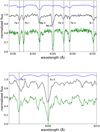 |
Fig. 2 Comparison of the spectra in the vicinity of the Nd and Eu lines between three A-type stars: the spectrum the star with a normal abundance, HD 186689 (top – blue), our target, KIC 10685175 (middle – black), and the spectrum of the known roAp star, α Cir (bottom – green). Strong spectral lines are marked with dashed black lines. The abscissa is wavelength in (Å) and the ordinate is normalized intensity. For clarity, the spectra of HD 186689 and α Cir have been shifted. |
4 The magnetic field of KIC 10685175
4.1 The surface magnetic field
High-resolution spectroscopic observations can be used to determine the mean magnetic field modulus, 〈B〉 (Mathys 1989), by measuring the wavelength shifts between the magnetically split components using the relation
 (1)
(1)
Here, λr, λb, and λ0 represent the wavelengths of the red and blue components, and the central wavelength, respectively; 𝑔 is the Landé factor, and k = 4.67×10⁻¹³ Å−1G−1.
The widely used magnetically sensitive doublet Fe II 6149 Å was inspected for the presence of magnetically split lines. However, as we show in Fig. 3, this line does not exhibit a magnetically split structure. We also inspected other magnetically sensitive lines that have large Landé factors (𝑔eff ≥1.5) and doublet patterns, such as Fe I 6336.82 Å (𝑔eff =2.0) and Cr II 5116.04 Å (𝑔eff =2.92), but no magnetically split pattern was detected. The relatively high v sin i for this star significantly inhibits the detection of magnetically split lines. Besides, the profile variation due to the spots can also contaminate the line splitting or broadening from the Zeeman effect, which makes the line splitting less likely to be detected.
4.2 The longitudinal magnetic field
The reduced circularly polarized observations provided the Stokes intensity, I, circular polarization – V – parameters, and diagnostic – N – spectra. The mean longitudinal magnetic field, 〈Bℓ〉, was determined through
![Mathematical equation: $\langle {B_\ell }\rangle = - 2.14 \times {10^{11}}{{{{\mathop \smallint \nolimits^ }^}vV(v)dv} \over {{\lambda _0}{g_{{\rm{eff}}}}c{{\mathop \smallint \nolimits^ }^}[{I_c} - I(v)]dv}}.$](/articles/aa/full_html/2024/11/aa51417-24/aa51417-24-eq3.png) (2)
(2)
Here, v is the velocity offset from the line center, and the unit is km s−1, while λ0 and 𝑔eff are the effective wavelength and the effective Landé factor used for normalization, respectively (Rees & Semel 1979; Donati et al. 1997).
The noise level was greatly reduced with the help of the least-squares deconvolution (LSD) technique (Donati et al. 1997; Folsom et al. 2018). In this technique, it is assumed that each spectral line can be described by the same profile with a different scale factor that depends on the central wavelength, line strength, and magnetic sensitivity.
The line list was constructed using the Vienna Atomic Line Database (VALD; Ryabchikova et al. 2015) assuming Teff = 8200 K and log 𝑔 = 4.4. All the lines were inspected to make sure that they are deeper than 5% of the continuum and not significantly blended with other lines. Lines contaminated by telluric absorption or located in hydrogen line wings were removed from the line list. The information about the selected line list is presented in Table 3.
In Fig. 4, we show for the line list constructed for all elements the LSD profiles of Stokes I, V, and diagnostic null. LSD profiles were calculated in the velocity range of −30 to 30 km s−1 using a step of 1 km s−1. The normalized Landé factor is 1.26, and the normalized wavelength of 4914 Å. We followed the generally adopted procedure of using the false alarm probability (FAP) based on reduced χ2 test statistics (Donati et al. 1992, 1997): the presence of a Zeeman signature is considered as a definite detection (DD) if FAP ≤ 10−5 , as a marginal detection (MD) if 10−5 < FAP ≤ 10−3, and as a non-detection (ND) if FAP > 10−3. The V spectrum exhibits a clear Zeeman feature, indicating the presence of a magnetic field. Using Eq. (2), the mean longitudinal magnetic field was calculated to be 〈Bℓ〉 = −226 ± 39 G. The FAP is listed in Table 3.
 |
Fig. 3 Combined spectrum (R = 81 000) of KIC 10685175 zoomed in on the spectral region containing the magnetically sensitive line Fe II 6149 Å. |
4.3 Comparison of the measured and predicted magnetic field strengths
In the recent study of Shi et al. (2020), it was suggested that KIC 10685175 possess a strong magnetic field with a dipole magnetic field strength of 6 kG. The theoretical pulsation model of Saio (2005) was used to compare the observations of KIC 10685175 with theoretical predictions. Following Stibbs (1950), and assuming a dipole magnetic field inclined by an angle, β, to the rotation axis, a polar magnetic field can be estimated through
 (3)
(3)
The limb darkening coefficient, u = 0.5, was extracted from Claret & Bloemen (2011), using log 𝑔 = 4.5, Teff = 8000 K, and a metallicity of Z = 0. The value Z was derived through Z =10[Fe/H]×Z⊙, where [Fe/H]=−0.4 and Z⊙=0.02. Using the mean longitudinal magnetic field strength, Bℓ = −226 ± 39 G, determined in the rotational phase Φ = 0.34, and the stellar inclination and the magnetic obliquity, (i,β) = (60°, 60°), from the pulsation model presented in Shi et al. (2020), we estimated the polar magnetic field to be 4.8 ± 0.8 kG. This is compatible with the theoretically predicted polar magnetic field of 6 kG within 3σ, supporting the theoretical model of Saio (2005).
Numbers of the lines in line lists and the mean longitudinal magnetic field calculated from different elements.
 |
Fig. 4 The profile of Stokes V, diagnostic null, and I (from top to bottom) calculated for KIC 10685175. |
5 Discussion and conclusion
Using two high-resolution spectroscopic spectra and one circularly polarized spectrum, we have studied the stellar parameters of the roAp star KIC 10685175 and measured its mean longitudinal magnetic field strength. Compared to chemically normal stars, KIC 10685175 exhibits chemical peculiarities such as an overabundance of Eu and Nd that is typical of magnetic Ap stars. The Fe lines, however, appear to be weaker than in other Ap stars with similar fundamental parameters.
Due to the lower number of available spectra, it is difficult to conclude whether chemical spots are present on the stellar surface. An inhomogeneous surface element distribution can be explored by considering the differences in magnetic field strengths obtained using line lists constructed for different elements. Assuming a dipolar magnetic field configuration, if a stronger mean longitudinal magnetic field is measured in the lines of a specific element, we can conclude that this element tends to form a spot closer to the magnetic pole. The results of the LSD technique applied to the line masks for Ca I, Cr II, Fe I, and Fe II are displayed in Fig. A.1 and the results of our measurements of the mean longitudinal magnetic field are presented in Table 3. Unfortunately, due to the low number of unblended lines belonging to the rare earth elements, no corresponding line lists have been constructed. Hümmerich et al. (2018) classified KIC 10685175 as A4V Eu. However, there are too few Eu lines visible in the spectrum to construct an Eu line mask.
As we show in Table 3, only the mean longitudinal magnetic field using Fe I lines is definitely detected and the result, Bℓ(Fe I)=−248 ± 47 G, is very close to the measurements obtained using all lines. This is reasonable because the number of Fe I lines dominates the line list. For Ca I, we obtained Bℓ(Ca I)=−115 ± 57 G, but the FAP indicates no detection. The magnetic fields for Fe II (−254 ± 55 G) and Cr II (−398 ± 105 G) are only marginally detected. The difference between the magnetic field strengths obtained for Cr II, Fe I, and Fe II is larger than 1σ. It is probably due to the inhomogeneous distribution of these elements, but is not significant enough for us to come to a solid conclusion.
Chemical spots on the surface of Ap stars usually cause significant variability of the spectral line profiles over the rotation period (Babcock 1958). To further test the possible presence of chemical spots on the surface of KIC 10685175, the LSD technique was applied for all three available observations to calculate the Stokes I profiles. Using the time zeropoint, T0=BJD 2 458 711.21391, and the rotation period, Prot = 3.1028 d, from Shi et al. (2020), both unpolarized spectra correspond to the rotation phases 0.92 and 0.93, respectively, and the polarized spectrum to the phase 0.34. For all three different rotation phases, the Stokes I profiles calculated for the line list containing all lines and those for the line lists constructed for different elements are presented in Fig. 5 and Fig. A.2. We also checked the Stokes I profiles for Nd and Pr, but only Nd III 6145 Å can be detected in all spectra. So, in Fig. A.2, we have compared the profiles of Nd III 6145 Å directly without calculating LSD profiles. No significant changes in the LSD Stokes I profiles are detected, although the profiles for Fe I calculated for the phase 0.34 show slightly flat-bottom profiles compared to those observed in other phases. As the rotation phase coverage of our data is rather poor, additional observations are needed to permit us to come to any conclusions about the surface inhomogeneous element distribution.
Despite the fact that magnetically split lines were not detected in our spectra, under the assumption of the dipolar topology of the global magnetic field, the strength of the measured mean longitudinal magnetic field, 〈Bℓ〉 = −226 ± 39 G, in combination with the already known stellar inclination and the magnetic obliquity, suggest that the polar magnetic field is 4.8 ± 0.8 kG. This polar field strength is consistent with the field strength predicted by the theoretical model of Saio (2005).
 |
Fig. 5 LSD Stokes I profiles calculated for all three available observations using all lines. The rotation phase is marked at the top of each panel. |
Acknowledgements
This work was funded by the National Natural Science Foundation of China (NSFC Grant Nos. 12090040, 12090042, 12090044, U1731108 and 11833002) and the National Key R&D Program of China (No. 2019YFA0405500). DWK acknowledges support from the Fundação para a Ciência e a Tecnologia (FCT) through national funds (2022.03993.PTDC). This work is based on data collected at the Canada-France-Hawaii Telescope, and also uses data from the VALD database, European Space Agency mission Gaia (http://www.cosmos.esa.int/Gaia), and the SIMBAD database. The observation time is obtained through the Telescope Access Program (TAP). Some of the observations in this paper were obtained with the Southern African Large Telescope (SALT) under proposal code 2017-1-SCI-023 (PI: Holdsworth). This work has made use of data products from the Guo Shou Jing Telescope (the Large Sky Area Multi Object Fibre Spectroscopic Telescope, LAMOST). LAMOST is a National Major Scientific Project built by the Chinese Academy of Sciences. Funding for the project has been provided by the National Development and Reform Commission. LAMOST is operated and managed by the National Astronomical Observatories, Chinese Academy of Sciences.
Appendix A Additional figure
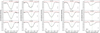 |
Fig. A.2 Same as Fig. 5 but for different elements. The rotation phase is marked at the top of each panel. For Nd III, the intensity profiles of 6145.07 Å are directly compared, instead of calculating LSD profiles. |
References
- Ammler-von Eiff, M., & Reiners, A. 2012, A&A, 542, A116 [NASA ADS] [CrossRef] [EDP Sciences] [Google Scholar]
- Anders, F., Khalatyan, A., Queiroz, A. B. A., et al. 2022, A&A, 658, A91 [NASA ADS] [CrossRef] [EDP Sciences] [Google Scholar]
- Babcock, H. W. 1958, ApJS, 3, 141 [Google Scholar]
- Balmforth, N. J., Cunha, M. S., Dolez, N., Gough, D. O., & Vauclair, S. 2001, MNRAS, 323, 362 [NASA ADS] [CrossRef] [Google Scholar]
- Bigot, L., & Kurtz, D. W. 2011, A&A, 536, A73 [NASA ADS] [CrossRef] [EDP Sciences] [Google Scholar]
- Blanco-Cuaresma, S. 2019, MNRAS, 486, 2075 [Google Scholar]
- Blanco-Cuaresma, S., Soubiran, C., Heiter, U., & Jofré, P. 2014, A&A, 569, A111 [CrossRef] [EDP Sciences] [Google Scholar]
- Borucki, W. J., Koch, D., Basri, G., et al. 2010, Science, 327, 977 [Google Scholar]
- Castelli, F., & Kurucz, R. L. 2004, IAU Symp. 210, Poster A20 [Google Scholar]
- Claret, A., & Bloemen, S. 2011, A&A, 529, A75 [NASA ADS] [CrossRef] [EDP Sciences] [Google Scholar]
- Cui, X.-Q., Zhao, Y.-H., Chu, Y.-Q., et al. 2012, Res. Astron. Astrophys., 12, 1197 [Google Scholar]
- Cunha, M. S. 2006, MNRAS, 365, 153 [NASA ADS] [CrossRef] [Google Scholar]
- Cunha, M. S., & Gough, D. 2000, MNRAS, 319, 1020 [CrossRef] [Google Scholar]
- Donati, J. F., Semel, M., & Rees, D. E. 1992, A&A, 265, 669 [Google Scholar]
- Donati, J. F., Semel, M., Carter, B. D., Rees, D. E., & Collier Cameron, A. 1997, MNRAS, 291, 658 [Google Scholar]
- Donati, J. F., Catala, C., Landstreet, J. D., & Petit, P. 2006, in Astronomical Society of the Pacific Conference Series, 358, Solar Polarization 4, eds. R. Casini, & B. W. Lites, 362 [NASA ADS] [Google Scholar]
- Dziembowski, W. A., & Goode, P. R. 1996, ApJ, 458, 338 [Google Scholar]
- Erspamer, D., & North, P. 2003, A&A, 398, 1121 [NASA ADS] [CrossRef] [EDP Sciences] [Google Scholar]
- Folsom, C. P., Bouvier, J., Petit, P., et al. 2018, MNRAS, 474, 4956 [NASA ADS] [CrossRef] [Google Scholar]
- Gaia Collaboration (Prusti, T., et al.) 2016, A&A, 595, A1 [NASA ADS] [CrossRef] [EDP Sciences] [Google Scholar]
- Gaia Collaboration (Brown, A. G. A., et al.) 2018, A&A, 616, A1 [NASA ADS] [CrossRef] [EDP Sciences] [Google Scholar]
- Gaia Collaboration (Vallenari, A., et al.) 2023, A&A, 674, A1 [NASA ADS] [CrossRef] [EDP Sciences] [Google Scholar]
- Ghazaryan, S., Alecian, G., & Hakobyan, A. A. 2018, MNRAS, 480, 2953 [NASA ADS] [CrossRef] [Google Scholar]
- Gray, R. O., Corbally, C. J., De Cat, P., et al. 2016, AJ, 151, 13 [Google Scholar]
- Grevesse, N., & Sauval, A. J. 1998, Space Sci. Rev., 85, 161 [Google Scholar]
- Holdsworth, D. L., & Brunsden, E. 2020, PASP, 132, 105001 [NASA ADS] [CrossRef] [Google Scholar]
- Holdsworth, D. L., Kurtz, D. W., Smalley, B., et al. 2016, MNRAS, 462, 876 [NASA ADS] [CrossRef] [Google Scholar]
- Holdsworth, D. L., Saio, H., Bowman, D. M., et al. 2018, MNRAS, 476, 601 [NASA ADS] [CrossRef] [Google Scholar]
- Huber, D., Silva Aguirre, V., Matthews, J. M., et al. 2014, ApJS, 211, 2 [NASA ADS] [CrossRef] [Google Scholar]
- Hümmerich, S., Mikulášek, Z., Paunzen, E., et al. 2018, A&A, 619, A98 [NASA ADS] [CrossRef] [EDP Sciences] [Google Scholar]
- Koch, D. G., Borucki, W. J., Basri, G., et al. 2010, ApJ, 713, L79 [Google Scholar]
- Kochukhov, O. 2003, A&A, 404, 669 [NASA ADS] [CrossRef] [EDP Sciences] [Google Scholar]
- Luo, A. L., Zhao, Y. H., Zhao, G., et al. 2022, VizieR Online Data Catalog: V/156 [Google Scholar]
- Mathys, G. 1989, Fund. Cosmic Phys., 13, 143 [Google Scholar]
- Matsuno, T., Starkenburg, E., Balbinot, E., & Helmi, A. 2024, A&A, 685, A59 [NASA ADS] [CrossRef] [EDP Sciences] [Google Scholar]
- Pinsonneault, M. H., An, D., Molenda-Zakowicz, J., et al. 2012, ApJS, 199, 30 [NASA ADS] [CrossRef] [Google Scholar]
- Preston, G. W. 1974, ARA&A, 12, 257 [Google Scholar]
- Rees, D. E., & Semel, M. D. 1979, A&A, 74, 1 [NASA ADS] [Google Scholar]
- Ricker, G. R., Winn, J. N., Vanderspek, R., et al. 2015, J. Astron. Telesc. Instrum. Syst., 1, 014003 [Google Scholar]
- Ryabchikova, T., Piskunov, N., Kurucz, R. L., et al. 2015, Phys. Scr., 90, 054005 [Google Scholar]
- Saio, H. 2005, MNRAS, 360, 1022 [NASA ADS] [CrossRef] [Google Scholar]
- Saio, H., & Gautschy, A. 2004, MNRAS, 350, 485 [NASA ADS] [CrossRef] [Google Scholar]
- Shi, F., Kurtz, D., Saio, H., Fu, J., & Zhang, H. 2020, ApJ, 901, 15 [NASA ADS] [CrossRef] [Google Scholar]
- Sneden, C., Bean, J., Ivans, I., Lucatello, S., & Sobeck, J. 2012, Astrophysics Source Code Library [record ascl:1202.009] [Google Scholar]
- Stibbs, D. W. N. 1950, MNRAS, 110, 395 [Google Scholar]
- Xiang, M., Rix, H.-W., Ting, Y.-S., et al. 2022, A&A, 662, A66 [NASA ADS] [CrossRef] [EDP Sciences] [Google Scholar]
- Zhao, G., Zhao, Y.-H., Chu, Y.-Q., Jing, Y.-P., & Deng, L.-C. 2012, Res. Astron. Astrophys., 12, 723 [NASA ADS] [CrossRef] [Google Scholar]
All Tables
Numbers of the lines in line lists and the mean longitudinal magnetic field calculated from different elements.
All Figures
|
Fig. 1 Phase-folded light curve of KIC 10685175. The positions of three spectral observations are marked as dotted lines in the figure. |
| In the text | |
|
Fig. 2 Comparison of the spectra in the vicinity of the Nd and Eu lines between three A-type stars: the spectrum the star with a normal abundance, HD 186689 (top – blue), our target, KIC 10685175 (middle – black), and the spectrum of the known roAp star, α Cir (bottom – green). Strong spectral lines are marked with dashed black lines. The abscissa is wavelength in (Å) and the ordinate is normalized intensity. For clarity, the spectra of HD 186689 and α Cir have been shifted. |
| In the text | |
|
Fig. 3 Combined spectrum (R = 81 000) of KIC 10685175 zoomed in on the spectral region containing the magnetically sensitive line Fe II 6149 Å. |
| In the text | |
|
Fig. 4 The profile of Stokes V, diagnostic null, and I (from top to bottom) calculated for KIC 10685175. |
| In the text | |
|
Fig. 5 LSD Stokes I profiles calculated for all three available observations using all lines. The rotation phase is marked at the top of each panel. |
| In the text | |
 |
Fig. A.1 Same as Fig. 4 but for different elements. |
| In the text | |
|
Fig. A.2 Same as Fig. 5 but for different elements. The rotation phase is marked at the top of each panel. For Nd III, the intensity profiles of 6145.07 Å are directly compared, instead of calculating LSD profiles. |
| In the text | |
Current usage metrics show cumulative count of Article Views (full-text article views including HTML views, PDF and ePub downloads, according to the available data) and Abstracts Views on Vision4Press platform.
Data correspond to usage on the plateform after 2015. The current usage metrics is available 48-96 hours after online publication and is updated daily on week days.
Initial download of the metrics may take a while.