© The Authors 2024

1. Introduction

Fluids in a turbulent regime transfer the energy of fluctuations across scales due to their non-linear interactions, in a process known as energy cascade. Non-linearities not only act upon the energy of fluctuations, but also on other turbulence properties as well. This enables the formation of multiple cascades in the system, with the development of one affecting that of another (Alexakis & Biferale 2018). Properties of incompressible magneto-hydrodynamic (MHD) fluid are strongly determined by three second-order (rugged) invariants: combined (kinetic plus magnetic) energy, and cross and magnetic helicities. While the magnetic helicity remains an ideal invariant even in the compressible Hall MHD, the presence of the Hall term couples the cross and kinetic helicities; a combination of the two, the mixed helicity (also called X helicity; see Pouquet & Yokoi 2022) is the ideal invariant appropriate for the incompressible Hall MHD. These ideal invariants are particularly relevant in turbulence. Cascade and dissipation of the combined energy is one of the central problems of (Hall) MHD turbulence and those processes are influenced by the different helicities, which in turn may exhibit analogous cascade and dissipation phenomena to the energy ones. All these processes constrain and change the dynamics of turbulent systems. For instance, cross helicity may reduce the energy cascade (Dobrowolny et al. 1980) and plays an important role in the generation of magnetic fields through turbulence dynamo processes (Yokoi 1999); it may also affect the repartition of heating between ions and electrons (Squire et al. 2023).

The solar wind exhibits important fluctuations of the magnetic field, plasma bulk velocity, and other quantities over a wide range of scales (Kiyani et al. 2015; Alexandrova et al. 2021). These fluctuations often have power-law-like spectral properties and are non-linearly coupled; the solar wind system is an example of a turbulent system in weakly collisional plasmas (Bruno & Carbone 2013). While slow solar wind streams have a weak average cross helicity (however see e.g. D’Amicis & Bruno 2015; Shi et al. 2021), fast solar wind streams have typically relatively strong average cross helicities. These high-cross helicity streams are also called Alfvénic streams as they exhibit important correlations or anti-correlations between the magnetic field and the plasma bulk velocities, which are characteristic of Alfvén waves (Belcher & Davis 1971; Grappin et al. 1991). Plasma turbulence in high-cross helicity streams and the behaviour of the combined energy and cross helicity are often studied in the incompressible MHD approximation and the energy and helicity is replaced by pseudo-energies in the terms of the Elsässer variables (combinations of the magnetic field in the Alfén units and the plasma bulk velocity; see Tu et al. 1989). In situ observations in the solar wind, as well as numerical simulations, indicate that the two pseudo-energies cascade in parallel, which means that the combined energy and cross helicity cascade in parallel. However, at variance with predictions of incompressible MHD (Dobrowolny et al. 1980), the combined energy in the solar wind decreases more slowly with the radial distance than the cross helicity, and consequently the relative cross helicity decreases. It is therefore important to determine the influence of compressive and non-ideal (Hall and kinetic) effects.

Compressive effects break the invariance of the combined energy and the mixed helicity, but the solar wind exhibits only weak density fluctuations (Shi et al. 2021), meaning that compressibility effects are likely not dominant in solar wind turbulence; the compressible MHD turbulence simulations of Montagud-Camps et al. (2022) behave qualitatively similar to incompressible simulations, again in contrast with observations. For weakly collisional solar-wind plasmas, it is also necessary to investigate the consequences of formation of non-Maxwellian particle distribution functions, which requires the tensor description of the particle pressure (Del Sarto et al. 2016). One of these consequences is the pressure-strain coupling, which appears to be very important, as it may work as an effective dissipation rate for the combined energy (Yang et al. 2017; Matthaeus et al. 2020). In this paper, we address the question how the pressure-strain effect influences the different helicities in order to complete our understanding of the rugged invariants in weakly collisional plasma turbulence. We analysed results of the two-dimensional pseudo-spectral hybrid simulation of decaying, high-cross helicity plasma turbulence. We used the Kármán-Howarth-Monin (KHM) equation (de Kármán & Howarth 1938; Politano & Pouquet 1998a,b) in the hybrid approximation for the energy (Hellinger et al. 2024) and we derived the equivalent equations for the helicities. The paper is organised as follows: In Section 2 we describe the pseudo-spectral hybrid code and in Section 3 we summarise the governing equations and their conservation properties. Section 4 presents the overall simulation results and in Section 5 we analyse the KHM properties of the energy (subsect. 5.1) and the cross, kinetic, and mixed helicities (subsect. 5.2). Finally, in Section 6 we summarise and discuss the simulation results. In the Appendix we complement our KHM results with spatial and spectral filtering techniques.

2. Numerical code

For the numerical simulation, we used the 2D pseudo-spectral version of the hybrid code based on the model of Matthews (1994). In this code, the electrons are considered as a massless charge-neutralising fluid, with a constant temperature, whereas ions are treated as particles. Ions have positions and velocities separated by half time steps and are advanced by the Boris scheme, which requires the fields to be known at a half time step ahead of the particle velocities. This is obtained by advancing the current density to this time (with only one computational pass through the particle data at each time step). The same grid is used for all the fields and their spatial derivatives, needed for the time advance (cf. Valentini et al. 2007), are calculated with the fast Fourier transform (Frigo & Johnson 2005). The particle contribution to the current density at the relevant nodes is evaluated with bilinear weighting followed by smoothing over three points. No smoothing is performed on the electromagnetic fields. A small resistivity is used in the Ohm’s law to avoid an accumulation of energy at small scales. The magnetic field is advanced in time with a modified midpoint method, which allows time substepping to advance the field.

The units and parameters of the simulation are as follows: units of space and time are the ion inertial length d_i = c/ω_pi and the (inverse of the) ion gyro-frequency Ω_i, respectively, where ω_pi = (n_pe²/m_pϵ₀)^1/2 is the proton plasma frequency. In these expressions, n_p and B₀ are the density of the plasma protons and magnitude of the initial magnetic field, respectively, while e and m_p are the proton electric charge and mass, respectively; and, finally c, ϵ₀, and μ₀ are the speed of light and the dielectric and magnetic permeabilities of vacuum, respectively. The spatial resolution is Δx = Δy = d_i/8. There are 16 384 particles per cell for protons; β_i = β_e = 0.5. The simulation box is in the x-y plane and is assumed to be periodic in both dimensions. The fields and moments are defined on a 2D grid with dimensions 2048 × 2048. The time step for the particle advance is dt = 0.01Ω_i⁻¹ while the magnetic field B is advanced with a smaller time step, dt_B = dt/20. (The vector potential A is initialised from the magnetic field assuming the Coulomb gauge and is then evolved in time in the code.) The background magnetic field B₀ is perpendicular to the simulation plane. Following Franci et al. (2015), we initialised the system with an isotropic 2D spectrum of modes with random phases, linear Alfvén polarisation (δB ⊥ B₀) over large scales k ≤ 0.1d_i⁻¹ with a flat 1D spectrum. The system initially has the (rms) amplitude of magnetic field fluctuations δB/B₀ = 0.3, and the relative cross helicity σ_c = 0.6. The magnetic and kinetic helicities are initially almost zero.

3. Governing equations

We investigated a system governed by the following equations for the plasma density ρ, the plasma mean velocity u, and the magnetic field B:

$$\begin{array}{cc}\hfill \frac{\partial \rho }{\partial t}+(\mathit{u}·\mathbf{\nabla })\rho & =-\rho \mathbf{\nabla }·\mathit{u},\hfill \end{array}$$(1)

$$\begin{array}{cc}\hfill \frac{\partial \mathit{u}}{\partial t}+(\mathit{u}·\mathbf{\nabla })\mathit{u}& =\frac{\mathit{J}\times \mathit{B}}{\rho }-\frac{\mathbf{\nabla }·\mathbf{P}}{\rho }\hfill \end{array}$$(2)

$$\begin{array}{cc}\hfill \frac{\partial \mathit{B}}{\partial t}& =\mathbf{\nabla }\times [(\mathit{u}-\mathit{j})\times \mathit{B}]+\eta {\mathrm{\nabla }}^2\mathit{B}.\hfill \end{array}$$(3)

Here P is the plasma pressure tensor, η is the electric resistivity, J is the electric current density, and j is the electric current density in velocity units, j = J/ρ_c = u − u_e (ρ_c and u_e being the charge density and the electron velocity, respectively). We assume SI units except for the magnetic permeability μ₀, which is set to one (SI results can be obtained by the rescaling B → Bμ₀^−1/2). Equation (3) (except the resistive term) can be derived taking moments of the Vlasov equation for protons and electrons, and assuming massless electrons. We added a resistive dissipation, as used in the hybrid code (cf. Hellinger et al. 2024).

We investigated properties of the different energies and helicities in electron–proton plasma in the hybrid approximation. For the sum of the (proton) kinetic (E_kin = ⟨ρ|u|²⟩/2) and the magnetic (E_mag = ⟨|B|²⟩/2) energies averaged over a closed volume (denoted by angle brackets ⟨ • ⟩) we obtained the following budget equation:

$$\begin{array}{c}\hfill {\partial }_t(E_{}\text{kin}+E_{}\text{mag})=-Q,\end{array}$$(4)

where Q = Q_η + ψ denotes the total (effective) dissipation rate consisting of the pressure-strain rate ψ = −⟨P : ∇u⟩, and the resistive dissipation rate Q_η = η⟨|J|²⟩. Following Kida & Orszag (1990), we defined a density-weighted velocity field w = ρ^1/2u and we represented the kinetic energy as a second-order positively definite quantity, E_kin = ⟨|w|²⟩/2.

For the averaged cross helicity (H_c = ⟨u ⋅ B⟩), we obtained the following equation:

$$\begin{array}{c}\hfill {\partial }_t{H}_c=-\langle \mathit{\omega }·(\mathit{j}\times \mathit{B})\rangle -{\psi }_{\mathit{Hc}}-{ϵ}_{\eta Hc},\end{array}$$(5)

where ω = ∇ × u is the vorticity field, ψ_Hc = −⟨P : ∇(B/ρ)⟩ is the cross helicity equivalent of the pressure-strain rate (generalisation of the pressure–dilation coupling; see Montagud-Camps et al. 2022), and ϵ_ηHc = η⟨ω ⋅ J⟩ is the cross helicity resistive dissipation rate. The first term on the right-hand side of Eq. (5) couples the cross helicity to the kinetic helicity.

For the (rescaled) kinetic helicity (H_k = m⟨u ⋅ ω⟩/(2e)), we derived the dynamic equation

$$\begin{array}{c}\hfill {\partial }_t{H}_k=\langle \mathit{\omega }·(\mathit{j}\times \mathit{B})\rangle -{\psi }_{\mathit{Hk}},\end{array}$$(6)

where ψ_Hk = −m⟨P : ∇(ω/ρ)⟩/e is the kinetic helicity equivalent of the pressure-strain rate. In the above formulas, we chose to represent the kinetic helicity with the renormalisation factor m/e, that is, the proton mass-to-charge ratio, in order to have the cross and kinetic helicities in the same units. The mixed helicity, the sum of the cross and (renormalised) kinetic helicities, H_x = H_c + H_k, is then an ideal invariant of the hybrid system, and behaves as

$$\begin{array}{c}\hfill {\partial }_t{H}_x=-{\psi }_{\mathit{Hc}}-{ϵ}_{\eta Hc}-{\psi }_{\mathit{Hk}}.\end{array}$$(7)

The magnetic helicity is a separate ideal invariant of Hall MHD as well as of the hybrid system. In this paper, we investigate properties of a simulated system with periodic boundary conditions and a background uniform magnetic field B₀ = ⟨B⟩. In this case, the vector potential A₀ generating B₀ = ∇ × A₀ is not periodic and affects the magnetic helicity conservation (Matthaeus & Goldstein 1982); we studied properties of the modified magnetic helicity H_m = ⟨A₁ ⋅ (B₁ + 2B₀)⟩, where B₁ and A₁ are the fluctuating components of the magnetic and vector potential fields, B₁ = B − B₀ and A₁ = A − A₀, respectively. For the averaged modified magnetic helicity, we obtained the following conservation properties:

$$\begin{array}{c}\hfill {\partial }_t{H}_m=-{ϵ}_{\mathit{Hm}},\end{array}$$(8)

where ϵ_Hm = 2η⟨B ⋅ J⟩ is the resistive dissipation rate.

4. Simulation results

Figure 1 shows the evolution of different quantities as a function of time. In the simulation, the proton kinetic energy E_kin and the magnetic energy E_mag oscillate with opposite phases, suggesting energy exchanges, but overall these two quantities decrease. On the other hand, the proton internal energy, E_int = 3⟨p⟩/2, increases (here p is the scalar pressure, p = tr(P), tr being the trace). This heating (energisation) is weak initially (tΩ_i ≲ 200) and gets progressively stronger as turbulence develops. The total energy E_tot = E_kin + E_int + E_mag slowly decreases owing to resistive dissipation because electrons are assumed to be massless and isothermal. This behaviour is seen in Fig. 1a, which displays the relative changes in the kinetic (ΔE_kin), magnetic (ΔE_mag), internal (ΔE_int), and total (ΔE_tot) energies. The proton energisation is driven by the pressure-strain coupling, which plays the role of an effective dissipation channel. Figure 1b displays the pressure-strain effective dissipation rate ψ and the resistive dissipation rate Q_η (dashed line). The pressure-strain rate ψ exhibits a large initial surge owing to a relaxation of the initial conditions and then slowly increases and saturates; ψ oscillates in time largely owing to compressive effects. The resistive dissipation rate Q_η slowly increases, exhibits a local maximum at around tΩ_i ≃ 240 (due to the onset of reconnection). The resistive dissipation rate reaches the maximum at tΩ_i ≃ 550 and slowly decreases thereafter.

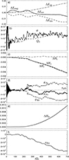Fig. 1. Evolution of different quantities as a function of time: (a) Relative changes in the kinetic energy ΔEkin (dashed line), magnetic energy ΔEmag (solid line), internal energy ΔEint (dash-dotted line), and total energy ΔEtot (dotted line), (b) resistive dissipation rate Qη (dashed line) and pressure-strain effective dissipation rate ψ (solid line), (c) relative changes in the kinetic helicity ΔHk (dash-dotted line), mixed helicity ΔHx (solid line), and cross helicity ΔHc (dashed line), (d) resistive cross-helicity dissipation rate ϵηHc (dotted line), pressure-strain effective cross-helicity dissipation rate ψHc (dashed line), pressure-strain effective mixed-helicity dissipation rate ψHx (solid line), and pressure-strain effective kinetic-helicity dissipation rate ψHk (dash-dotted line), (e) relative change in the magnetic helicity ΔHm, and (f) resistive magnetic-helicity dissipation rate ϵHm.

The cross helicity H_c decreases with time, initially slowly, and later (tΩ_i ≳ 200) the decrease is faster and approximately linear in time; the kinetic helicity H_k very slightly increases at the beginning (from its nearly zero initial value) and remains roughly constant later on (tΩ_i ≳ 200); consequently, the mixed helicity H_x = H_c + H_k closely follows the evolution of the cross helicity H_c. This is shown in Fig. 1c, which displays the evolution of the relative changes in the cross (ΔH_c), mixed (ΔH_x), and kinetic (ΔH_k) helicities. We expected this evolution of the different helicities to be driven by the respective (effective) dissipation rates. Figure 1d shows the resistive cross-helicity dissipation rate ϵ_ηHc, and the equivalents of the pressure-strain effective dissipation: the cross-helicity rate ψ_Hc, the kinetic-helicity rate ψ_Hk, and the mixed-helicity rate ψ_Hx. The resistive cross-helicity dissipation rate is negligible but the cross-helicity pressure-strain rate ψ_Hc is strong and reaches a roughly constant value at tΩ_i ≳ 240, which is compatible with the rate of decrease in the cross helicity. We interpret ψ_Hc as an effective dissipation rate of the cross helicity. On the other hand, the kinetic-helicity ψ_Hk and the mixed-helicity ψ_Hx rates become negative for later times (tΩ_i ≳ 300), which is at variance with the time evolution of H_k and H_x; interpretations of the terms ψ_Hk and ψ_Hx are unclear. The pressure-strain terms ψ_Hc and ψ_Hk are dominated by incompressive fluctuations, and their compressive components ⟨p(B ⋅ ∇)ρ⁻¹⟩ and ⟨p(ω ⋅ ∇)ρ⁻¹⟩ are negligible due to small density variations (here p is the scalar pressure, p = tr(P), tr being the trace). The combined energy and the cross helicity decrease in time but the latter process is slower; consequently the relative cross helicity increases with time.

Finally, the (modified) magnetic helicity increases with time in a quadratic manner as displayed in Fig. 1e, which shows the relative change in this quantity (ΔH_m). This evolution is driven by the resistive magnetic-helicity dissipation rate ϵ_Hm, which becomes negative and decreases approximately linearly for tΩ_i ≳ 200 (see Fig. 1f). In summary, Figure 1 indicates that, for tΩ_i ≳ 550, the different dissipation rates are relatively constant, a property which is expected in a fully developed turbulence system. Once this state is attained in a free decaying simulation, temporal variations of the fluctuating quantities can be considered negligible (we test this expectation using the KHM equations in Section 5).

During the evolution, the kinetic and magnetic energies spread over a wide range of scales and similar evolution is observed for the cross helicity. Figure 2 shows their omnidirectional spectral properties at tΩ_i = 700: Figure 2a displays power spectral densities of B and w fields, P_B and P_w, respectively. These power spectral densities exhibit a power-law-like behaviour at large scales (with a slope somewhat less steep than −5/3) and they steepen at small scales, P_w at around kd_i ≃ 1 and P_B at around kd_i ≃ 3. The kinetic spectral density P_w becomes dominated by the noise for about kd_i ≳ 6, whereas the magnetic spectral density P_B seems to be affected by the noise for kd_i ≳ 20.

Figure 2b shows co-spectra of the cross helicity P_Hc and the (absolute value of the) kinetic helicity P_Hk. P_Hc exhibits a power-law like behaviour at large scales with a slope similar to that of the energy power spectral densities and steepens somewhere between kd_i ≃ 1 and kd_i ≃ 3, which are the spectral break points of P_w and P_B. The kinetic-helicity co-spectrum P_Hk oscillates between positive and negative values and constitutes a small fraction of P_Hc at large scales and at small scales P_Hk becomes comparable to P_Hc; for kd_i ≳ 6, both quantities are dominated by the noise. As the magnetic helicity remains small during the whole simulation, we did not investigate its spectral or spatial decomposition properties.

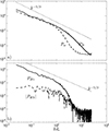Fig. 2. Omnidirectional spectral properties of different quantities at tΩi = 700: (a) Power spectral densities of (solid) the magnetic field B, PB (solid), and compensated proton velocity field w, Pw (dashed), as a function of k normalised to di. (b) Cross helicity co-spectrum PHc (solid) and (absolute value of) kinetic helicity co-spectrum PHk (dashed) as a function of k. The dotted lines show a spectrum ∝k−5/3 for comparison.

5. The Kármán-Howarth-Monin equations

To understand cross-scale transfers (cascades), exchanges, and dissipations of energies and helicities, we analysed the hybrid simulation results using the corresponding KHM equations. We started with the combined energy.

5.1. Energy

We characterised the spatial scale decomposition of the kinetic and magnetic (and their sum) energies using the second-order structure functions:

$$\begin{array}{c}\hfill S_w=\frac{1}{4}\langle {|\delta \mathit{w}|}^2\rangle ,S_B=\frac{1}{4}\langle {|\delta \mathit{B}|}^2\rangle ,\text{and}S=S_w+S_B,\end{array}$$

where the deltas denote increments of the corresponding quantities; for example, δw = w(x + l)−w(x), with x being the position and l the separation (lag) vector. For the second-order structure function, S, we obtain (Hellinger et al. 2024)

$$\begin{array}{c}\hfill {\partial }_{t}S=K_{}\text{MHD}+K_{}\text{Hall}-\Psi -D,\end{array}$$(9)

where K_MHD and K_Hall are the MHD and Hall non-linear cross-scale transfer (cascade) rates, respectively, $\Psi$ represents the pressure-strain effect, and D accounts for the effects of resistive dissipation. We expressed the cascade rates K_MHD and K_Hall (as well as $\Psi$ and D) in the following form:

$$\begin{array}{cc}\hfill K_{}\text{MHD}& =-\frac{1}{2}\langle \delta \mathit{w}·\delta [(\mathit{u}·\mathbf{\nabla })\mathit{w}+\frac{1}{2}\mathit{w}(\mathbf{\nabla }·\mathit{u})]\rangle \hfill \\ \hfill & -\frac{1}{2}\langle \delta \mathit{w}·\delta \left(\frac{\mathit{J}\times \mathit{B}}{\sqrt{\rho }}\right)\rangle +\frac{1}{2}\langle \delta \mathit{J}·\delta (\mathit{u}\times \mathit{B})\rangle \hfill \end{array}$$(10)

$$\begin{array}{cc}\hfill K_{}\text{Hall}& =-\frac{1}{2}\langle \delta \mathit{J}·\delta (\mathit{j}\times \mathit{B})\rangle \hfill \end{array}$$(11)

$$\begin{array}{cc}\hfill \Psi & =-\frac{1}{2}\langle \delta \mathit{w}·\delta \left(\frac{\mathbf{\nabla }·\mathbf{P}}{\sqrt{\rho }}\right)\rangle \hfill \end{array}$$(12)

$$\begin{array}{cc}\hfill D& =\frac{1}{2}\eta \langle {|\delta \mathit{J}|}^2\rangle =Q_{\eta }-\frac{1}{2}\eta {\mathrm{\nabla }}^2{S}_B.\hfill \end{array}$$(13)

The KHM equation constitutes a cross-scale energy conservation equation; we define the validity test O as

$$\begin{array}{c}\hfill O=-{\partial }_{t}S+K_{}\text{MHD}+K_{}\text{Hall}-\Psi -D,\end{array}$$(14)

which measures the error of the code owing to numerical issues. Figure 3 displays the isotropised energy KHM analysis of the simulation results at the end of the simulation, tΩ_i = 700. Figure 3 shows the validity test O and the different contributing terms, −∂_tS​, K_MHD, K_Hall, $-\Psi$, and −D (normalised to the total effective dissipation rate Q) as a function of the scale separation l = |l| (normalised to d_i). The KHM Equation (9) is relatively well satisfied (|O|/Q ≲ 10 %); this error is connected with the noise level owing to the particle-in-cell scheme. The energy decay ∂_tS​ is strong at large scales l ≳ 10d_i, but becomes less important and is negligible somewhat below l = d_i. The MHD cascade rate is around zero at large scales and becomes important at intermediate scales (6d_i ≳ l ≳ 1d_i), where it reaches a maximum value of about the dissipation rate Q. At small scales, part of the cascade continues via the Hall term and K_Hall attains a maximum value of about 20% of Q; at these scales, the resistive dissipation and the pressure-strain interaction are also active.

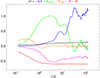Fig. 3. Isotropised energy KHM analysis at tΩi = 700: Validity test O (black line) as a function of l along with the different contributing terms: decay rate −∂tS (blue), MHD cascade rate KMHD (green), Hall cascade rate KHall (orange), resistive dissipation rate −D (red), and pressure-strain rate $-\Psi$ (magenta). All the quantities are normalised to the effective total dissipation rate Q.

Figure 3 shows the properties of well-developed decaying turbulence (see Fig. 3 of Hellinger et al. 2024). The combined energy decays at large scales, cascades at intermediate scales, and dissipates at small scales. As the KHM equation remains relatively well satisfied throughout the entire simulation, including the turbulence onset, we can analyse the temporal evolution of each KHM term at all times. We can determine which term or process dominates (at a given scale) during the onset and once the cascade is fully developed. Figure 4 shows the evolution of the isotropised KHM results, the different contributing terms as a function of time, and the separation scale l normalised to the total effective dissipation rate Q (averaged over the time interval 600 ≤ tΩ_i ≤ 700). Figure 4 demonstrates that the features of well-developed turbulence seen in Fig. 3 only appear at later times. During an initial phase (0 ≤ tΩ_i ≤ 200), the system is governed by ∂_tS ≃ K_MHD, and increasingly small scales are generated through the (MHD) non-linear coupling as ∂_tS is positive at intermediate scales. At later times (for about tΩ_i ≲ 550), ∂_tS becomes negative, monotonically decreasing with l as expected. As the energy transfer towards smaller scales continues, the resistive and the effective pressure-strain dissipation effects gradually appear (their behaviour corresponds to the evolution of the resistive Q_η and pressure-strain rates ψ in Fig. 1b). The Hall term gradually sets in around 180 ≲ tΩ_i ≲ 230.

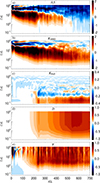Fig. 4. Evolution of isotropised energy KHM results. Shown are the different KHM terms as a function of time t and l: (a) decay rate ∂tS, (b) MHD cascade rate KMHD, (c) Hall cascade rate KHall, (d) resistive dissipation rate D, and (e) pressure-strain rate $\Psi$. All the quantities are normalised to the effective total dissipation rate Q (averaged over 600 ≤ tΩi ≤ 700).

5.2. Cross and kinetic helicities

Next we continued with the cross, kinetic, and mixed helicities. First, we characterised the cross helicity using a second-order structure function (cf. Banerjee & Galtier 2016, 2017) as

$$\begin{array}{c}\hfill S_{\mathit{Hc}}=\frac{1}{2}\langle \delta \mathit{u}·\delta \mathit{B}\rangle .\end{array}$$(15)

For S​_Hc we get the following dynamic KHM equation:

$$\begin{array}{c}\hfill {\partial }_t{S}_{\mathit{Hc}}=K_{\text{MHD}Hc}+K_{\text{Hall}Hc}-{\Psi }_{\mathit{Hc}}-D_{\mathit{Hc}},\end{array}$$(16)

where

$$\begin{array}{cc}\hfill K_{\text{MHD}Hc}& =-\frac{1}{2}\langle \delta \mathit{B}·\delta [(\mathit{u}·\mathbf{\nabla })\mathit{u}]\rangle +\frac{1}{2}\langle \delta \mathit{B}·\delta \left(\frac{\mathit{J}\times \mathit{B}}{\rho }\right)\rangle \hfill \\ \hfill & +\frac{1}{2}\langle \delta \mathit{\omega }·\delta (\mathit{u}\times \mathit{B})\rangle \hfill \end{array}$$(17)

$$\begin{array}{cc}\hfill K_{\text{Hall}Hc}& =-\frac{1}{2}\langle \delta \mathit{\omega }·\delta (\mathit{j}\times \mathit{B})\rangle \hfill \end{array}$$(18)

$$\begin{array}{cc}\hfill D_{\mathit{Hc}}& =\frac{\eta }{2}\langle \delta \mathit{\omega }·\delta \mathit{J}\rangle \hfill \end{array}$$(19)

$$\begin{array}{cc}\hfill {\Psi }_{\mathit{Hc}}& =\frac{1}{2}\langle \delta \mathit{B}·\delta \left(\frac{\mathbf{\nabla }·\mathbf{P}}{\rho }\right)\rangle .\hfill \end{array}$$(20)

Here, K_MHDHc and K_HallHc represent the MHD and Hall non-linear coupling terms, respectively, D_Hc accounts for the effects of resistive dissipation, whereas $\Psi$ characterises the cross-helicity equivalent of the pressure-strain effect.

Similarly, we define a second-order structure function for the kinetic helicity:

$$\begin{array}{c}\hfill S_{\mathit{Hk}}=\frac{m}{4e}\langle \delta \mathit{u}·\delta \mathit{\omega }\rangle .\end{array}$$(21)

For S​_Hk, the KHM equation reads

$$\begin{array}{c}\hfill {\partial }_t{S}_{\mathit{Hk}}=K_{\text{MHD}Hk}+K_{\text{Hall}Hk}-{\Psi }_{\mathit{Hk}},\end{array}$$(22)

where

$$\begin{array}{cc}\hfill K_{\text{MHD}Hk}& =-\frac{m}{2e}\langle \delta \mathit{\omega }·\delta [(\mathit{u}·\mathbf{\nabla })\mathit{u}]\rangle ,\hfill \end{array}$$(23)

$$\begin{array}{cc}\hfill K_{\text{Hall}Hk}& =-K_{\text{Hall}Hc},\hfill \end{array}$$(24)

$$\begin{array}{cc}\hfill {\Psi }_{\mathit{Hk}}& =\frac{m}{2e}\langle \delta \mathit{\omega }·\delta \left(\frac{\mathbf{\nabla }·\mathbf{P}}{\rho }\right)\rangle .\hfill \end{array}$$(25)

Here, analogously to the cross helicity, K_MHDHk and K_HallHk represent the MHD and Hall non-linear coupling terms, respectively, and ${\Psi }_{\mathit{Hk}}$ characterises the kinetic-helicity equivalent of the pressure-strain effect.

Finally, for the mixed helicity, we define a second-order structure function as a sum of the two previous ones,

$$\begin{array}{c}\hfill S_{\mathit{Hx}}=S_{\mathit{Hc}}+S_{\mathit{Hk}},\end{array}$$(26)

and we obtain the corresponding KHM equation (again as a sum of the two previous ones):

$$\begin{array}{c}\hfill {\partial }_t{S}_{\mathit{Hx}}=K_{\text{MHD}Hx}-{\Psi }_{\mathit{Hx}}-D_{\mathit{Hc}},\end{array}$$(27)

where

$$\begin{array}{cc}\hfill K_{\mathit{Hx}}& =K_{\text{MHD}Hc}+K_{\text{MHD}Hk}\hfill \end{array}$$(28)

$$\begin{array}{cc}\hfill {\Psi }_{\mathit{Hx}}& ={\Psi }_{\mathit{Hc}}+{\Psi }_{\mathit{Hk}}.\hfill \end{array}$$(29)

In the mixed-helicity KHM equation, K_Hx represents the MHD non-linear coupling term (the Hall contribution cancels out), D_Hc remains the cross-helicity resistive term, and ${\Psi }_{\mathit{Hx}}$ characterises the mixed-helicity equivalent of the pressure-strain effect.

Starting with the mixed helicity, we define the validity test O_Hx,

$$\begin{array}{c}\hfill O_{\mathit{Hx}}=-{\partial }_t{S}_{\mathit{Hx}}+K_{\mathit{Hx}}-{\Psi }_{\mathit{Hx}}-D_{\mathit{Hc}},\end{array}$$(30)

as in the energy case. Figure 5 displays the isotropised mixed-helicity KHM analysis of the simulation results at the end of the simulation, tΩ_i = 700, showing the validity test O_Hx and the different contributing terms (−∂_tS​_Hx, K_Hx, $-{\Psi }_{\mathit{Hx}}$, −D_Hc) as a function of the scale separation l=. These quantities are normalised to the total effective dissipation rate ϵ_Hc = ϵ_ηHc + ψ_Hc, a sum of the cross-helicity resistive and pressure-strain rates. As for the energy, the mixed-helicity KHM Eq. (27) is relatively well satisfied (|O_Hx|/ϵ_Hc ≲ 5 %).

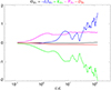Fig. 5. Isotropised mixed-helicity KHM analysis at tΩi = 700: Validity test OHx (black line) as a function of l along with the different contributing terms: decay rate −∂tS​Hx (blue), MHD term KHx (green), resistive dissipation rate −DHc (red), and pressure-strain rate $-{\Psi }_{\mathit{Hx}}$ (magenta). All the quantities are normalised to the effective total (cross-helicity) dissipation rate ϵHc.

Figure 5 exhibits a very different behaviour from that seen in Fig. 3 for the energy. The decay term ∂_tS​_Hx is important (and negative) at large scales. The dissipation term D_Hc is positive but small, and the resistive dissipation of cross and mixed helicities is weak. While ∂_tS​_Hx and D_Hc behave similarly to the energy counterparts, K_Hx and ${\Psi }_{\mathit{Hx}}$ are of opposite sign. The mixed-helicity pressure-strain term ${\Psi }_{\mathit{Hx}}$ has a negative sign, which suggests that the pressure-strain coupling generates the mixed helicity at small scales. The non-linear term K_Hx also has a negative sign, which may indicate an inverse cascade of the mixed helicity. These two suggestions are at variance with the overall decrease in the mixed helicity; consequently, we cannot interpret K_Hx as the cascade rate and ${\Psi }_{\mathit{Hx}}$ as the effective dissipation rate of the mixed helicity.

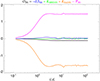Fig. 6. Isotropised kinetic-helicity KHM analysis at tΩi = 700: Validity test OHk (black line) as a function of l along with the different contributing terms: the decay rate −∂tS​Hk (blue), the MHD cascade rate KMHDHk (green), the Hall cascade rate KHallHk (orange), and the pressure-strain rate $-{\Psi }_{\mathit{Hk}}$ (magenta). All the quantities are normalised to the effective total (cross-helicity) dissipation rate ϵHc.

To better understand the behaviour of the mixed helicity, we looked at its two contributions, H_c and H_k, separately. We started with the kinetic helicity KHM Equation (22), defining the corresponding validity test O_Hk,

$$\begin{array}{c}\hfill O_{\mathit{Hk}}=-{\partial }_t{S}_{\mathit{Hk}}+K_{\text{MHD}Hk}+K_{\text{Hall}Hk}-{\Psi }_{\mathit{Hk}}.\end{array}$$(31)

Figure 6 displays the isotropised kinetic-helicity KHM analysis of the simulation results at the end of the simulation, tΩ_i = 700; it shows the validity test O_Hk and the different contributing terms, −∂_tS​_Hk, K_MHDHx, K_HallHx, and $-{\Psi }_{\mathit{Hk}}$ (normalised to the total effective dissipation rate ϵ_Hc) as a function of the scale separation l. The kinetic-helicity KHM equation is well satisfied (|O_Hk|/ϵ_Hc ≲ 10 %), but the behaviours of the different terms are very different from the energy KHM results in Fig. 3. The decay term ∂_tS​_Hk and the MHD coupling term K_MHDHx are negligible; this is in agreement with the evolution of the kinetic helicity, which is roughly constant. In contrast, the Hall coupling term K_HallHx and the pressure-strain term ${\Psi }_{\mathit{Hk}}$ are strong and mostly compensate each other,

$$\begin{array}{c}\hfill K_{\text{Hall}Hk}\simeq {\Psi }_{\mathit{Hk}}.\end{array}$$(32)

Therefore, the Hall term couples to the kinetic-helicity pressure-strain term.

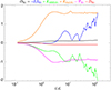Fig. 7. Isotropised cross-helicity KHM analysis at tΩi = 700: Validity test OHc (black line) as a function of l along with the different contributing terms: the decay rate −∂tS​Hc (blue), the MHD term KMHDHc (green), the Hall term KHallHc (orange), the resistive dissipation rate −DHc (red), and the pressure-strain rate $-{\Psi }_{\mathit{Hc}}$ (magenta). All the quantities are normalised to the effective total (cross-helicity) dissipation rate ϵHc.

We continued with the cross-helicity KHM Equation (16): we define the corresponding validity test O_Hc,

$$\begin{array}{c}\hfill O_{\mathit{Hc}}=-{\partial }_t{S}_{\mathit{Hc}}+K_{\text{MHD}Hc}+K_{\text{Hall}Hc}-{\Psi }_{\mathit{Hk}}-D_{\mathit{Hc}}.\end{array}$$(33)

Figure 7 displays the isotropised cross-helicity KHM analysis of the simulation results at the end of the simulation, tΩ_i = 700; it shows the validity test O_Hc and the different contributing terms, −∂_tS​_Hc, K_MHDHc, K_HallHc, $-{\Psi }_{\mathit{Hc}}$, and −D_Hc, as a function of the scale separation l. The cross-helicity KHM equation is relatively well satisfied (|O_Hc|/ϵ_Hc ≲ 15 %). The results of Fig. 7 become somewhat similar to those of the energy KHM results of Fig. 3: the decay term ∂_tS​_Hc is negative and dominates at large scales; and the resistive and the cross-helicity pressure-strain rates behave as dissipation channels and are important at small scales. However, the MHD and Hall coupling terms remain strange. Nevertheless, when we combine them into one term, K_Hc = K_MHDHc + K_HallHc, the resulting quantity exhibits an analogous behaviour to the energy cascade rate (see Fig. 3).

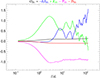Fig. 8. Rearranged isotropised cross-helicity KHM analysis of Fig. 7: Validity test OHc (black line), decay rate −∂tS​Hc (blue), MHD+Hall term KHc (green), resistive dissipation rate −DHc (red), and pressure-strain rate $-{\Psi }_{\mathit{Hc}}$ (magenta) as a function of l. All the quantities are normalised to the effective total (cross-helicity) dissipation rate ϵHc.

Figure 8 repeats the results of Fig. 7 but combines the MHD and Hall contributions into one term, K_Hc. This indicates that K_Hc describes the total (MHD+Hall) cascade rate of the cross helicity. Figure 8 indicates that the cross helicity decays at large scales, cascades at intermediate scales, and dissipates at small scales via the resistive and effective pressure-strain dissipation effects, at least at the end of simulation. We used the cross-helicity KHM equation to look at the development of the system. Figure 9 shows the evolution of the isotropised KHM results, the different contributing terms as a function of time, and the separation scale l normalised to the total effective dissipation rate ϵ_Hc (averaged over the time interval 600 ≤ tΩ_i ≤ 700). Figure 9 reveals a very similar behaviour to the energy properties in Fig. 4. During the initial phase (0 ≤ tΩ_i ≤ 200), the system is governed by ∂_tS​_Hc ≃ K_Hc, and increasingly small scales are generated through the (MHD) non-linear coupling as ∂_tS​_Hc is positive at intermediate scales. At later times (for about tΩ_i ≲ 550), ∂_tS​_Hc becomes mostly negative and negligible at small scales. As the energy transfer towards smaller scales continues, the resistive dissipation and more importantly the pressure-strain effective dissipation gradually appear (corresponding to the evolution of the resistive ϵ_ηHc and pressure-strain rates ψ_Hc in Fig. 1d).

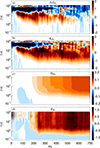Fig. 9. Evolution of isotropised cross-helicity KHM results. Shown are the different KHM terms as a function of time t and l: (a) decay rate ∂tS​Hc, (b) MHD+Hall cascade rate KHc, (c) resistive dissipation rate DHc, and (d) pressure-strain rate ${\Psi }_{\mathit{Hc}}$. All the quantities are normalised to the effective total dissipation rate ϵHc (averaged over 600 ≤ Ωi ≤ 700).

6. Discussion

In this paper we present an investigation of 2D decaying plasma turbulence in a weakly collisional plasma with an out-of-plane background magnetic field using a pseudo-spectral hybrid code. The plasma system is initialised with substantial fluctuating kinetic and magnetic energies as well as cross helicity at relatively large scales; these initial fluctuations exhibit no overall magnetic or kinetic helicities. We analyse the simulation results using the KHM equation for the combined (kinetic plus magnetic) energy, and cross, kinetic, and mixed helicities. These different KHM equations, which characterise the cross-scale conservation of the given quantity, are well satisfied. These code properties are partly attributable to the pseudo-spectral scheme, which improves the cross-scale conservation properties compared to a finite-difference scheme. The KHM results show that the combined energy, which is initially distributed at large scales, transfers to smaller scales owing to the non-linear MHD term (and later the Hall one). After a transient period, a fully developed turbulent system arises, where the energy decays at large scales, cascades at intermediate scales, and is dissipated at small scales via the resistive term and the pressure-strain term; this system plays the role of an effective dissipation mechanism. These results agree with previous hybrid simulation results (Hellinger et al. 2022, 2024).

The properties of the cross, kinetic, and mixed helicities are more complicated. In the hybrid approximation, we expected the mixed helicity (combination of the cross and kinetic helicities) to be the relevant quantity, which decays, cascades, and dissipates. However, the simulation results show that the cross helicity is the relevant quantity in weakly collisional plasmas. The corresponding KHM equation indicates that the cross helicity behaves analogously to the combined energy: it decays at large scales, cascades via the MHD and Hall non-linear coupling at intermediate scales, and dissipates at small scales via the resistive term and, more importantly, via the cross helicity equivalent of the pressure-strain term, which again plays a role of an effective dissipation mechanism.

The combined energy and the cross helicity decrease over time, but the latter process is slower, and consequently the relative cross helicity increases. This is in agreement with the theoretical incompressible MHD expectations and numerical simulations (e.g. Dobrowolny et al. 1980; Montagud-Camps et al. 2022), but is at variance with observations (Bavassano et al. 1998). This effect may be related to large-scale gradients in the solar wind due to its expansion (Grappin et al. 2022) and/or velocity shears (Roberts et al. 1992); we note that, assuming homogeneity, these effects can be included in the KHM equation (Wan et al. 2009; Stawarz et al. 2011; Hellinger et al. 2013).

The magnetic helicity is a separate ideal invariant in the hybrid system (similarly to the Hall MHD case; see Pouquet & Yokoi 2022). In the simulation, the magnetic helicity is initially negligible and is scantily generated via the resistive term (as the magnetic helicity is not a positively definite quantity, this term may lead to its production). We did not observe any coupling between the magnetic and cross helicities, in agreement with theoretical expectations. We also derived and analysed the KHM equation for the magnetic helicity; these results indicate that the magnetic helicity does not exhibit any cascade (not shown here). We investigated a system where the mixed and magnetic helicities are not coupled, but in a more general situation it is necessary to investigate the generalised (canonical) helicity, that is, a combination of the mixed and magnetic helicities (cf. Pouquet & Yokoi 2022). In such a situation, there may be coupling between the cross and magnetic helicities, which could lead to a reduction of the energy cascade, a phenomenon called helicity barrier (Meyrand et al. 2021). Squire et al. (2023) interpreted some hybrid simulation results as being a consequence of the helicity barrier. Our results, however, show that the helicity barrier is not relevant in hybrid (or Hall MHD) systems.

In this work, we used the KHM equations to analyse numerical simulation results for the properties of the energy and the cross helicity. Based on the similarities between the KHM results for the two quantities, we conclude that, even though the cross helicity is not an ideal invariant, it is this quantity that decays, cascades, and dissipates in parallel with the combined energy. As our results could simply be due to some peculiar properties of the KHM approach, we investigated analogous spectral-transfer and coarse-graining approaches (see Appendices A and B). We obtained equivalent results for the energy and the cross helicity, allowing us to conclude that our results are robust. However, we investigated only one 2D simulation with a particular set of parameters; more simulations are needed to study the roles of the various plasma and turbulence parameters. In particular, it would be interesting to check how different values of magnetic helicity (and its cascade) influence properties of plasma turbulence (cf. Stribling et al. 1995). Furthermore, in the simulation, the initial kinetic helicity was negligible and remained negligible during the whole simulation. It is not clear what would happen if the simulation were to start with a strong kinetic helicity. This work also needs to be extended to three dimensions to account for the anisotropy induced by the background magnetic field (Verdini et al. 2015; Montagud-Camps et al. 2022; Hellinger et al. 2024). It is also necessary to study a fully kinetic regime; the electron pressure strain effect may act at relatively large scales for the energy (Yang et al. 2022; Manzini et al. 2024) and may influence the evolution of the cross helicity.

In conclusion, this paper we show that the dynamics of cross helicity in weakly collisional plasmas is strongly affected over a wide range of scales (even well above ion scales) by the Hall and pressure-strain physics. Observational tests of these results are challenging; the relevant quantities contain the vorticity field, which is impossible to measure with just one spacecraft. The incompressible MHD KHM equation is often used to estimate energy and cross-helicity cascade rates from in situ spacecraft measurements in the solar wind (Sorriso-Valvo et al. 2007; MacBride et al. 2008; Stawarz et al. 2009; Marino & Sorriso-Valvo 2023). Our results, along with those of previous studies, show that at large scales this approximation is sufficient for the energy; the Hall correction appears at the ion scale (Bandyopadhyay et al. 2020) and the pressure-strain effect for the energy also becomes important at around this scale (Yang et al. 2022; Manzini et al. 2024). On the other hand, our results indicate that the MHD estimates of the cross-helicity cascade rate are inadequate in the solar wind; in our simulation, the cross-helicity MHD cascade rate is weaker than the Hall cascade rate and they even have the opposite sign.

Acknowledgments

This work was supported by the Ministry of Education, Youth and Sports of the Czech Republic through the e-INFRA CZ (ID:90254). The authors thank T. Tullio for a continuous enriching support and acknowledge useful discussions with A. Verdini, S. Landi, L. Matteini, Emanuele Papini, and L. Franci.

References

Appendix A: Energy

A.1. Spectral transfer approach

Another possibility how to quantify the turbulence properties is the spectral approach (cf. Mininni et al. 2007; Grete et al. 2017). We characterised the combined energy by a low-pass filtered quantity (Hellinger et al. 2021, 2024)

$$\begin{array}{cc}\hfill E_k& =\frac{1}{2}\sum _{|{\mathit{k}}^{\prime }|\le k}(|\widehat{\mathit{w}}{|}^2+{|\widehat{\mathit{B}}|}^2),\hfill \end{array}$$(A.1)

where the wide hat denotes the Fourier transform. For the spectrally-decomposed quantity E_k we obtained the following dynamic equation

$$\begin{array}{c}\hfill {\partial }_t{E}_k+S_{\text{MHD}k}+S_{\text{Hall}k}=-{\mathrm{\Psi }}_k-D_k,\end{array}$$(A.2)

where S​_MHDk and S​_Hallk represent the MHD and Hall energy transfer rates, respectively; Ψ_k describes the pressure-strain effect; and D_k is the resistive dissipation rate for modes with wave-vector magnitudes smaller than or equal to k. They can be expressed as

$$\begin{array}{cc}\hfill S_{\text{MHD}k}& =\mathfrak{R}\sum _{|{\mathit{k}}^{\prime }|\le k}[{\widehat{\mathit{w}}}^{\ast }·\widehat{(\mathit{u}·\mathbf{\nabla })\mathit{w}}+\frac{1}{2}{\widehat{\mathit{w}}}^{\ast }·\widehat{\mathit{w}(\mathbf{\nabla }·\mathit{u})}\hfill \\ \hfill & -{\widehat{\mathit{w}}}^{\ast }·\widehat{{\rho }^{-1/2}\mathit{J}\times \mathit{B}}-{\widehat{\mathit{B}}}^{\ast }·\widehat{\mathbf{\nabla }\times (\mathit{u}\times \mathit{B})}],\hfill \end{array}$$(A.3)

$$\begin{array}{cc}\hfill S_{\text{Hall}k}& =\mathfrak{R}\sum _{|{\mathit{k}}^{\prime }|\le k}{\widehat{\mathit{B}}}^{\ast }·\widehat{\mathbf{\nabla }\times (\mathit{j}\times \mathit{B})},\hfill \end{array}$$(A.4)

$$\begin{array}{cc}\hfill {\mathrm{\Psi }}_k& =\mathfrak{R}\sum _{|{\mathit{k}}^{\prime }|\le k}{\widehat{\mathit{w}}}^{\ast }·\widehat{{\rho }^{-1/2}\mathbf{\nabla }·\mathbf{P}},\hfill \end{array}$$(A.5)

$$\begin{array}{cc}\hfill D_k& =\eta \sum _{|{\mathit{k}}^{\prime }|\le k}|{\mathit{k}}^{\prime }{|}^2{|\widehat{\mathit{B}}|}^2.\hfill \end{array}$$(A.6)

In these expression the asterisk denotes the complex conjugate, and ℜ denotes the real part. For fully developed turbulence S​_MHDk and S​_Hallk are the MHD and Hall cascade rates, respectively.

Similarly to the KHM case, we defined the validity test of the spectral transfer (ST) equation, Eq. (A.2), as

$$\begin{array}{c}\hfill O_k={\partial }_t{E}_k+S_{\text{MHD}k}+S_{\text{Hall}k}+{\mathrm{\Psi }}_k+D_k.\end{array}$$(A.7)

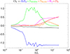Fig. A.1. Spectral transfer (ST) analysis of the combined energy, the validity test of the isotropic ST Ok, Eq. (A.7), as a function of k at tΩi = 700 (black line) along with the different contributing terms: decay rate ∂tEk (blue), MHD cascade rate S​MHDk (green), Hall cascade rate S​Hallk (orange), resistive dissipation rate Dk (red), and pressure-strain rate Ψk (magenta). All the quantities are given in units of the total (effective) dissipation rate Q.

Figure A.1 shows the ST validity test O_k and the contributing terms as functions of k at tΩ_i = 700 The ST equation (A.2) is relatively well satisfied (|O_k|/Q ≲ 14 %). Figure A.1 quantifies the turbulence properties, the energy decays at large scales, cascades at intermediate scales, and at small scales the cascade partly continues via the Hall term and partly is dissipated by the resistive and pressure-strain effects. The ST results in Fig. A.1 are quantitatively equivalent to the corresponding KHM results (see Fig. 3) through the inverse proportionality $kl=\sqrt{2}$. Using this relationship we got

$$\begin{array}{c}\hfill S_{\text{MHD}k}\simeq K_{}\text{MHD},S_{\text{Hall}k}\simeq K_{}\text{Hall}.\end{array}$$(A.8)

The other terms exhibit a complementarity properties; the ST approach is by construction (spectral) low-pass filter whereas the KHM approach exhibits rather high-pass (or spatial low-pass) filter behaviour (see Hellinger et al. 2021, 2024).

A.2. Coarse-graining approach

An alternative way how to analyse the turbulence properties is the spatial filtering (Eyink & Aluie 2009; Aluie 2011; Manzini et al. 2022). In this approach the scale decomposition of the combined energy is done using a spatial filter (coarse graining)

$$\begin{array}{c}\hfill E_l=\frac{1}{2}\langle \overline{\rho }|\stackrel{\sim }{\mathit{u}}{|}^2+{|\overline{\mathit{B}}|}^2\rangle \end{array}$$(A.9)

where the line denotes a spatial filtering

$$\begin{array}{c}\hfill {\overline{\mathit{a}}}_l(\mathit{x})=\int {\mathrm{d}}^{2}x{G}_l(\mathit{r})\mathit{a}(\mathit{x}+\mathit{r})\end{array}$$(A.10)

and the tilde denotes the corresponding density-weighted or Favre filtering (Favre 1969)

$$\begin{array}{c}\hfill {\stackrel{\sim }{\mathit{a}}}_l=\frac{{\overline{\rho \mathit{u}}}_l}{{\overline{\rho }}_l}.\end{array}$$(A.11)

For the filtered energy we obtained this dynamic equation

$$\begin{array}{c}\hfill {\partial }_t{E}_l+{\mathrm{\Pi }}_{\text{MHD}l}+{\mathrm{\Pi }}_{\text{Hall}l}=-{\mathrm{\Phi }}_l-{\mathcal{D}}_l\end{array}$$(A.12)

where Π_MHDl and Π_Halll represent the MHD and Hall energy transfer rates, respectively; Φ_l and 𝒟_l describe the pressure-strain and resistive dissipation effects, respectively. These terms can be expressed as

$$\begin{array}{cc}\hfill {\mathrm{\Pi }}_{\text{MHD}l}& =\langle \mathbf{\nabla }\stackrel{\sim }{\mathit{u}}:\overline{\rho }\stackrel{\sim }{\mathit{\tau }}\rangle -\langle \stackrel{\sim }{\mathit{u}}·\overline{\mathit{J}\times \mathit{B}}\rangle -\langle \overline{\mathit{J}}·\overline{(\mathit{u}\times \mathit{B})}\rangle \hfill \end{array}$$(A.13)

$$\begin{array}{cc}\hfill {\mathrm{\Pi }}_{\text{Hall}l}& =\langle \overline{\mathit{J}}·\overline{(\mathit{j}\times \mathit{B})}\rangle \hfill \end{array}$$(A.14)

$$\begin{array}{cc}\hfill {\mathrm{\Phi }}_l& =-\langle \mathbf{\nabla }\stackrel{\sim }{\mathit{u}}:\overline{\mathbf{P}}\rangle \hfill \end{array}$$(A.15)

$$\begin{array}{cc}\hfill {\mathcal{D}}_l& =\eta \langle |\overline{\mathit{J}}{|}^2\rangle \hfill \end{array}$$(A.16)

where $\stackrel{\sim }{\mathit{\tau }}=\stackrel{\sim }{\mathit{u}}\stackrel{\sim }{\mathit{u}}-\stackrel{\sim }{\mathit{u}\mathit{u}}$. As before we defined the validity test of the coarse-graining (CG) equation, Eq. (A.12), as

$$\begin{array}{c}\hfill {\mathcal{O}}_l={\partial }_t{E}_l+{\mathrm{\Pi }}_{\text{MHD}l}+{\mathrm{\Pi }}_{\text{Hall}l}+{\mathrm{\Phi }}_l+{\mathcal{D}}_l\end{array}$$(A.17)

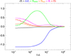Fig. A.2. Coarse-graining (CG) analysis of the combined energy: Validity test of the isotropic CG 𝒪l, Eq. (A.17), as a function of k at tΩi = 700(black line) along with the different contributing terms: decay rate ∂tEl (blue), MHD cascade rate ΠMHDl (green), Hall cascade rate ΠHalll (orange), resistive dissipation rate 𝒟l (red), and pressure-strain rate Φl (magenta). All the quantities are given in units of the total (effective) dissipation rate Q.

Figure A.2 shows results of the coarse-graining for the spatial low-pass filter using the normalized boxcar window function. The CG validity test is relatively well satisfied (|𝒪_l|/Q ≲ 10 %); the respective errors of the KHM, ST, and CG approaches are comparable. Figure A.2 repeats the turbulence picture we saw in the KHM and ST approaches, the energy decays at large scales, cascades at intermediate scales, and at small scales the cascade partly continues via the Hall term and partly is dissipated by the resistive and pressure-strain effects. For the spatial low-pass filter and the same separation and filter scale l we obtained quantitatively equivalent MHD and Hall cascade rates compared to the KHM equation (and, consequently, compared to the ST equation as we saw in the previous subsection):

$$\begin{array}{c}\hfill {\mathrm{\Pi }}_{\text{MHD}l}\simeq K_{}\text{MHD},{\mathrm{\Pi }}_{\text{Hall}l}\simeq K_{}\text{Hall}.\end{array}$$(A.18)

The other respective terms in the CG and KHM approaches exhibit a complementarity behaviour, which is similar to that of the ST approach in subsection A.1. We note that it is possible to use the spectral filtering in a way analogical to the CG approach (Arró et al. 2022). It is possible to use spectral low-pass filters, which lead to an inverse dependence of the different quantities on l (i.e. l → −l).

Appendix B: Cross helicity

B.1. Spectral transfer

For the spectral scale decomposition of the cross helicity we chosen

$$\begin{array}{cc}\hfill H_{\mathit{ck}}& =\mathfrak{R}\sum _{|{\mathit{k}}^{\prime }|\le k}({\widehat{\mathit{u}}}^{\ast }·\widehat{{\mathit{B}}_1})\hfill \end{array}$$(B.1)

In analogy with the KHM equation (where the increment representation losses the information about the background magnetic field B₀) we used the fluctuating magnetic field B₁ = B − B₀. For H_ck we obtained the following dynamic equation

$$\begin{array}{c}\hfill {\partial }_t{H}_{\mathit{ck}}+S_{\mathit{Hck}}=-{\mathrm{\Psi }}_{\mathit{Hck}}-D_{\mathit{Hck}},\end{array}$$(B.2)

where S​_Hck represents the (joint MHD and Hall) cross helicity transfer rate, and Ψ_Hck and D_Hck describe the pressure-strain and resistive dissipation effects, respectively. These terms can be expressed as

$$\begin{array}{cc}\hfill S_{\mathit{Hck}}& =\mathfrak{R}\sum _{|{\mathit{k}}^{\prime }|\le k}[{\widehat{{\mathit{B}}_1}}^{\ast }·\widehat{(\mathit{u}·\mathbf{\nabla })\mathit{u}}-{\widehat{{\mathit{B}}_1}}^{\ast }·\widehat{\frac{\mathit{J}\times \mathit{B}}{\rho }}\hfill \\ \hfill & -{\widehat{\mathit{\omega }}}^{\ast }·\widehat{\mathit{u}\times \mathit{B}}+{\widehat{\mathit{\omega }}}^{\ast }·\widehat{\mathit{j}\times \mathit{B}}]\hfill \end{array}$$(B.3)

$$\begin{array}{cc}\hfill {\mathrm{\Psi }}_{\mathit{Hck}}& =\mathfrak{R}\sum _{|{\mathit{k}}^{\prime }|\le k}{\widehat{{\mathit{B}}_1}}^{\ast }·\widehat{\frac{\mathbf{\nabla }·\mathbf{P}}{\rho }}\hfill \end{array}$$(B.4)

$$\begin{array}{cc}\hfill D_{\mathit{Hck}}& =\eta \mathfrak{R}\sum _{|{\mathit{k}}^{\prime }|\le k}{|{\mathit{k}}^{\prime }|}^2{\widehat{\mathit{u}}}^{\ast }·\widehat{\mathit{B}}\hfill \end{array}$$(B.5)

Here again we defined the validity test of the ST cross-helicity equation (B.2) as

$$\begin{array}{c}\hfill O_{\mathit{Hck}}={\partial }_t{H}_{\mathit{ck}}+S_{\mathit{Hck}}+{\mathrm{\Psi }}_{\mathit{Hck}}+D_{\mathit{Hck}}.\end{array}$$(B.6)

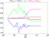Fig. B.1. ST analysis of the cross helicity: Validity test of the isotropic ST OHck, Eq. (B.6), as a function of k at tΩi = 700 (black line) along with the different contributing terms: decay rate ∂tHck (blue), cascade rate S​Hck (green), resistive dissipation rate DHck (red), and pressure-strain rate ΨkHc (magenta). All the quantities are given in units of the total (effective) cross-helicity dissipation rate ϵHc.

Figure B.1 shows that the cross helicity ST equation (B.2) is relatively well satisfied (|O_Hck|/ϵ_Hc ≲ 15%). In the Fig. B.1 we recovered the KHM results, the cross helicity decays at large scales, cascades at intermediate scales, and at small scales it is dissipated by the resistive and pressure-strain effects, with the latter process being the dominant one. Similarly to the case of the energy ST and KHM equations the cross helicity ST and KHM approaches give equivalent cascade rates

$$\begin{array}{c}\hfill S_{\mathit{Hck}}\simeq K_{}\text{Hc}\end{array}$$(B.7)

for $kl=\sqrt{2}$. The other terms have again complementary behaviour.

B.2. Coarse graining

For the scale-decomposition of the cross helicity we choose the following filtered quantity

$$\begin{array}{c}\hfill H_{\mathit{cl}}=\langle \overline{{\mathit{B}}_1}·\overline{\mathit{u}}\rangle .\end{array}$$(B.8)

For the coarse-grained cross helicity H_cl we obtained this dynamic equation

$$\begin{array}{c}\hfill {\partial }_t{H}_{\mathit{cl}}+{\mathrm{\Pi }}_{\mathit{Hcl}}=-{\mathrm{\Phi }}_{\mathit{Hcl}}-{\mathcal{D}}_{\mathit{Hcl}}.\end{array}$$(B.9)

where Π_Hcl represents the cross helicity transfer rate, and Φ_Hcl and 𝒟_Hcl describe the pressure-strain and resistive dissipation effects, respectively. These terms can be expressed as

$$\begin{array}{cc}\hfill {\mathrm{\Pi }}_{\mathit{Hcl}}& =\langle \overline{{\mathit{B}}_1}·\overline{(\mathit{u}·\mathbf{\nabla })\mathit{u}}\rangle -\langle \overline{{\mathit{B}}_1}·\overline{\frac{\mathit{J}\times \mathit{B}}{\rho }}\rangle -\langle \overline{\mathit{\omega }}·\overline{\mathit{u}\times \mathit{B}}\rangle \hfill \\ \hfill & +\langle \overline{\mathit{\omega }}·\overline{\mathit{j}\times \mathit{B}}\rangle \hfill \end{array}$$(B.10)

$$\begin{array}{cc}\hfill {\mathrm{\Phi }}_{\mathit{Hcl}}& =\langle \overline{{\mathit{B}}_1}·\overline{\frac{\mathbf{\nabla }·\mathbf{P}}{\rho }}\rangle \hfill \end{array}$$(B.11)

$$\begin{array}{cc}\hfill {\mathcal{D}}_{\mathit{Hcl}}& =\eta \langle \overline{\mathit{\omega }}·\overline{\mathit{J}}\rangle \hfill \end{array}$$(B.12)

As before, we defined the validity test of the CG cross-helicity equation (B.9) as

$$\begin{array}{c}\hfill {\mathcal{O}}_{\mathit{Hcl}}={\partial }_t{H}_{\mathit{cl}}+{\mathrm{\Pi }}_{\mathit{Hcl}}+{\mathrm{\Phi }}_{\mathit{Hcl}}+{\mathcal{D}}_{\mathit{Hcl}}\end{array}$$(B.13)

Figure B.2 shows that the cross helicity CG equation is relatively well satisfied (|𝒪_Hcl|/ϵ_Hc ≲ 16%). Figure B.2 again repeats the same information seen in the corresponding KHM and ST analyses: the cross helicity decays at large scales, cascades at intermediate scales, and at small scales it is dissipated by the resistive and pressure-strain effects. The KHM and CG approaches give quantitatively similar results, for the cascade rates

$$\begin{array}{c}\hfill {\mathrm{\Pi }}_{\mathit{Hcl}}\simeq K_{\mathit{Hc}}.\end{array}$$(B.14)

The other respective terms in the CG and KHM approaches exhibit a complementarity behaviour, which is similar to that of the ST approach in subsection B.1.

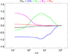Fig. B.2. CG analysis of the cross helicity: Validity test of the isotropic CG 𝒪Hcl, Eq. (B.13), as a function of k at tΩi = 700 (black line) along with the different contributing terms: decay rate ∂tHcl (blue), MHD cascade rate ΠHcl (green), resistive dissipation rate 𝒟Hcl (red), and pressure-strain rate ΦHcl (magenta). All the quantities are given in units of the total (effective) cross-helicity dissipation rate ϵHc.

All Figures

Fig. 1. Evolution of different quantities as a function of time: (a) Relative changes in the kinetic energy ΔEkin (dashed line), magnetic energy ΔEmag (solid line), internal energy ΔEint (dash-dotted line), and total energy ΔEtot (dotted line), (b) resistive dissipation rate Qη (dashed line) and pressure-strain effective dissipation rate ψ (solid line), (c) relative changes in the kinetic helicity ΔHk (dash-dotted line), mixed helicity ΔHx (solid line), and cross helicity ΔHc (dashed line), (d) resistive cross-helicity dissipation rate ϵηHc (dotted line), pressure-strain effective cross-helicity dissipation rate ψHc (dashed line), pressure-strain effective mixed-helicity dissipation rate ψHx (solid line), and pressure-strain effective kinetic-helicity dissipation rate ψHk (dash-dotted line), (e) relative change in the magnetic helicity ΔHm, and (f) resistive magnetic-helicity dissipation rate ϵHm.

In the text

Fig. 2. Omnidirectional spectral properties of different quantities at tΩi = 700: (a) Power spectral densities of (solid) the magnetic field B, PB (solid), and compensated proton velocity field w, Pw (dashed), as a function of k normalised to di. (b) Cross helicity co-spectrum PHc (solid) and (absolute value of) kinetic helicity co-spectrum PHk (dashed) as a function of k. The dotted lines show a spectrum ∝k−5/3 for comparison.

In the text

	Fig. 3. Isotropised energy KHM analysis at tΩi = 700: Validity test O (black line) as a function of l along with the different contributing terms: decay rate −∂tS (blue), MHD cascade rate KMHD (green), Hall cascade rate KHall (orange), resistive dissipation rate −D (red), and pressure-strain rate $-\Psi$ (magenta). All the quantities are normalised to the effective total dissipation rate Q.
In the text

	Fig. 4. Evolution of isotropised energy KHM results. Shown are the different KHM terms as a function of time t and l: (a) decay rate ∂tS, (b) MHD cascade rate KMHD, (c) Hall cascade rate KHall, (d) resistive dissipation rate D, and (e) pressure-strain rate $\Psi$. All the quantities are normalised to the effective total dissipation rate Q (averaged over 600 ≤ tΩi ≤ 700).
In the text

Fig. 5. Isotropised mixed-helicity KHM analysis at tΩi = 700: Validity test OHx (black line) as a function of l along with the different contributing terms: decay rate −∂tS​Hx (blue), MHD term KHx (green), resistive dissipation rate −DHc (red), and pressure-strain rate $-{\Psi }_{\mathit{Hx}}$ (magenta). All the quantities are normalised to the effective total (cross-helicity) dissipation rate ϵHc.

In the text

Fig. 6. Isotropised kinetic-helicity KHM analysis at tΩi = 700: Validity test OHk (black line) as a function of l along with the different contributing terms: the decay rate −∂tS​Hk (blue), the MHD cascade rate KMHDHk (green), the Hall cascade rate KHallHk (orange), and the pressure-strain rate $-{\Psi }_{\mathit{Hk}}$ (magenta). All the quantities are normalised to the effective total (cross-helicity) dissipation rate ϵHc.

In the text

Fig. 7. Isotropised cross-helicity KHM analysis at tΩi = 700: Validity test OHc (black line) as a function of l along with the different contributing terms: the decay rate −∂tS​Hc (blue), the MHD term KMHDHc (green), the Hall term KHallHc (orange), the resistive dissipation rate −DHc (red), and the pressure-strain rate $-{\Psi }_{\mathit{Hc}}$ (magenta). All the quantities are normalised to the effective total (cross-helicity) dissipation rate ϵHc.

In the text

	Fig. 8. Rearranged isotropised cross-helicity KHM analysis of Fig. 7: Validity test OHc (black line), decay rate −∂tS​Hc (blue), MHD+Hall term KHc (green), resistive dissipation rate −DHc (red), and pressure-strain rate $-{\Psi }_{\mathit{Hc}}$ (magenta) as a function of l. All the quantities are normalised to the effective total (cross-helicity) dissipation rate ϵHc.
In the text

	Fig. 9. Evolution of isotropised cross-helicity KHM results. Shown are the different KHM terms as a function of time t and l: (a) decay rate ∂tS​Hc, (b) MHD+Hall cascade rate KHc, (c) resistive dissipation rate DHc, and (d) pressure-strain rate ${\Psi }_{\mathit{Hc}}$. All the quantities are normalised to the effective total dissipation rate ϵHc (averaged over 600 ≤ Ωi ≤ 700).
In the text

Fig. A.1. Spectral transfer (ST) analysis of the combined energy, the validity test of the isotropic ST Ok, Eq. (A.7), as a function of k at tΩi = 700 (black line) along with the different contributing terms: decay rate ∂tEk (blue), MHD cascade rate S​MHDk (green), Hall cascade rate S​Hallk (orange), resistive dissipation rate Dk (red), and pressure-strain rate Ψk (magenta). All the quantities are given in units of the total (effective) dissipation rate Q.

In the text

Fig. A.2. Coarse-graining (CG) analysis of the combined energy: Validity test of the isotropic CG 𝒪l, Eq. (A.17), as a function of k at tΩi = 700(black line) along with the different contributing terms: decay rate ∂tEl (blue), MHD cascade rate ΠMHDl (green), Hall cascade rate ΠHalll (orange), resistive dissipation rate 𝒟l (red), and pressure-strain rate Φl (magenta). All the quantities are given in units of the total (effective) dissipation rate Q.

In the text

Fig. B.1. ST analysis of the cross helicity: Validity test of the isotropic ST OHck, Eq. (B.6), as a function of k at tΩi = 700 (black line) along with the different contributing terms: decay rate ∂tHck (blue), cascade rate S​Hck (green), resistive dissipation rate DHck (red), and pressure-strain rate ΨkHc (magenta). All the quantities are given in units of the total (effective) cross-helicity dissipation rate ϵHc.

In the text

Fig. B.2. CG analysis of the cross helicity: Validity test of the isotropic CG 𝒪Hcl, Eq. (B.13), as a function of k at tΩi = 700 (black line) along with the different contributing terms: decay rate ∂tHcl (blue), MHD cascade rate ΠHcl (green), resistive dissipation rate 𝒟Hcl (red), and pressure-strain rate ΦHcl (magenta). All the quantities are given in units of the total (effective) cross-helicity dissipation rate ϵHc.

In the text

References

- Alexakis, A., & Biferale, L. 2018, Phys. Rep., 767, 1 [CrossRef] [Google Scholar]
- Alexandrova, O., Jagarlamudi, V. K., Hellinger, P., et al. 2021, Phys. Rev. E, 103, 063202 [NASA ADS] [CrossRef] [Google Scholar]
- Aluie, H. 2011, Phys. Rev. Lett., 106, 174502 [NASA ADS] [CrossRef] [Google Scholar]
- Arró, G., Califano, F., & Lapenta, G. 2022, A&A, 668, A33 [NASA ADS] [CrossRef] [EDP Sciences] [Google Scholar]
- Bandyopadhyay, R., Sorriso-Valvo, L., Chasapis, A., et al. 2020, Phys. Rev. Lett., 124, 225101 [CrossRef] [Google Scholar]
- Banerjee, S., & Galtier, S. 2016, Phys. Rev. E, 93, 033120 [NASA ADS] [CrossRef] [Google Scholar]
- Banerjee, S., & Galtier, S. 2017, J. Phys. A, 50, 015501 [NASA ADS] [CrossRef] [Google Scholar]
- Bavassano, B., Pietropaolo, E., & Bruno, R. 1998, J. Geophys Res., 103, 6521 [NASA ADS] [CrossRef] [Google Scholar]
- Belcher, J. W., & Davis, L., Jr 1971, J. Geophys Res., 76, 3534 [NASA ADS] [CrossRef] [Google Scholar]
- Bruno, R., & Carbone, V. 2013, LRSP, 10, 2 [NASA ADS] [Google Scholar]
- D’Amicis, R., & Bruno, R. 2015, ApJ, 805, 84 [Google Scholar]
- de Kármán, T., & Howarth, L. 1938, Proc. R. Soc. London Ser. A, 164, 192 [CrossRef] [Google Scholar]
- Del Sarto, D., Pegoraro, F., & Califano, F. 2016, Phys. Rev. E, 93, 053203 [CrossRef] [Google Scholar]
- Dobrowolny, M., Mangeney, A., & Veltri, P. 1980, Phys. Rev. Lett., 45, 144 [CrossRef] [Google Scholar]
- Eyink, G. L., & Aluie, H. 2009, Phys. Fluids, 21, 115107 [NASA ADS] [CrossRef] [Google Scholar]
- Favre, A. 1969, Problems of Hydrodynamic and Continuum Mechanics (Philadelphia: SIAM), 231 [Google Scholar]
- Franci, L., Landi, S., Matteini, L., Verdini, A., & Hellinger, P. 2015, ApJ, 812, 21 [NASA ADS] [CrossRef] [Google Scholar]
- Frigo, M., & Johnson, S. G. 2005, Proc. IEEE, 93, 216 [Google Scholar]
- Grappin, R., Velli, M., & Mangeney, A. 1991, Ann. Geophys., 9, 416 [Google Scholar]
- Grappin, R., Verdini, A., & Müller, W. C. 2022, ApJ, 933, 246 [NASA ADS] [CrossRef] [Google Scholar]
- Grete, P., O’Shea, B. W., Beckwith, K., Schmidt, W., & Christlieb, A. 2017, Phys. Plasmas, 24, 092311 [NASA ADS] [CrossRef] [Google Scholar]
- Hellinger, P., Trávníček, P. M., Štverák, Š., Matteini, L., & Velli, M. 2013, J. Geophys Res., 118, 1351 [NASA ADS] [CrossRef] [Google Scholar]
- Hellinger, P., Papini, E., Verdini, A., et al. 2021, ApJ, 917, 101 [NASA ADS] [CrossRef] [Google Scholar]
- Hellinger, P., Montagud-Camps, V., Franci, L., et al. 2022, ApJ, 930, 48 [NASA ADS] [CrossRef] [Google Scholar]
- Hellinger, P., Verdini, A., Montagud-Camps, V., et al. 2024, A&A, 684, A120 [NASA ADS] [CrossRef] [EDP Sciences] [Google Scholar]
- Kida, S., & Orszag, S. A. 1990, J. Sci. Comput., 5, 85 [NASA ADS] [CrossRef] [Google Scholar]
- Kiyani, K. H., Osman, K. T., & Chapman, S. C. 2015, Phil. Trans. R. Soc. A, 373, 20140155 [Google Scholar]
- MacBride, B. T., Smith, C. W., & Forman, M. A. 2008, ApJ, 679, 1644 [NASA ADS] [CrossRef] [Google Scholar]
- Manzini, D., Sahraoui, F., Califano, F., & Ferrand, R. 2022, Phys. Rev. E, 106, 035202 [NASA ADS] [CrossRef] [Google Scholar]
- Manzini, D., Sahraoui, F., & Califano, F. 2024, Phys. Rev. Lett., 132, 235201 [NASA ADS] [CrossRef] [Google Scholar]
- Marino, R., & Sorriso-Valvo, L. 2023, Phys. Rep., 1006, 1 [NASA ADS] [CrossRef] [Google Scholar]
- Matthaeus, W. H., & Goldstein, M. L. 1982, J. Geophys Res., 87, 6011 [NASA ADS] [CrossRef] [Google Scholar]
- Matthaeus, W. H., Yang, Y., Wan, M., et al. 2020, ApJ, 891, 101 [NASA ADS] [CrossRef] [Google Scholar]
- Matthews, A. 1994, JCoPh, 112, 102 [NASA ADS] [Google Scholar]
- Meyrand, R., Squire, J., Schekochihin, A. A., & Dorland, W. 2021, J. Plasma Phys., 87, 535870301 [CrossRef] [Google Scholar]
- Mininni, P. D., Alexakis, A., & Pouquet, A. 2007, J. Plasma Phys., 73, 377 [NASA ADS] [CrossRef] [Google Scholar]
- Montagud-Camps, V., Hellinger, P., Verdini, A., et al. 2022, ApJ, 938, 90 [NASA ADS] [CrossRef] [Google Scholar]
- Politano, H., & Pouquet, A. 1998a, Geophys. Res. Lett., 25, 273 [NASA ADS] [CrossRef] [Google Scholar]
- Politano, H., & Pouquet, A. 1998b, Phys. Rev. E, 57, R21 [CrossRef] [Google Scholar]
- Pouquet, A., & Yokoi, N. 2022, Phil. Trans. R. Soc. A, 380, 20210087 [CrossRef] [Google Scholar]
- Roberts, D. A., Goldstein, M. L., Matthaeus, W. H., & Ghosh, S. 1992, J. Geophys Res., 97, 17115 [NASA ADS] [CrossRef] [Google Scholar]
- Shi, C., Velli, M., Panasenco, O., et al. 2021, ApJ, 650, A21 [Google Scholar]
- Sorriso-Valvo, L., Marino, R., Carbone, V., et al. 2007, Phys. Rev. Lett., 99, 115001 [CrossRef] [Google Scholar]
- Squire, J., Meyrand, R., & Kunz, M. W. 2023, ApJ, 957, L30 [NASA ADS] [CrossRef] [Google Scholar]
- Stawarz, J. E., Smith, C. W., Vasquez, B. J., Forman, M. A., & MacBride, B. T. 2009, ApJ, 697, 1119 [NASA ADS] [CrossRef] [Google Scholar]
- Stawarz, J. E., Vasquez, B. J., Smith, C. W., Forman, M. A., & Klewicki, J. 2011, ApJ, 736, 44 [NASA ADS] [CrossRef] [Google Scholar]
- Stribling, T., Matthaeus, W. H., & Oughton, S. 1995, Phys. Plasmas, 2, 1437 [NASA ADS] [CrossRef] [Google Scholar]
- Tu, C. Y., Marsch, E., & Thieme, K. M. 1989, J. Geophys Res., 94, 11739 [NASA ADS] [CrossRef] [Google Scholar]
- Valentini, F., Trávníček, P., Califano, F., Hellinger, P., & Mangeney, A. 2007, JCoPh, 225, 753 [NASA ADS] [Google Scholar]
- Verdini, A., Grappin, R., Hellinger, P., Landi, S., & Müller, W. C. 2015, ApJ, 804, 119 [NASA ADS] [CrossRef] [Google Scholar]
- Wan, M., Servidio, S., Oughton, S., & Matthaeus, W. H. 2009, Phys. Plasmas, 16, 090703 [NASA ADS] [CrossRef] [Google Scholar]
- Yang, Y., Matthaeus, W. H., Parashar, T. N., et al. 2017, Phys. Plasmas, 24, 072306 [NASA ADS] [CrossRef] [Google Scholar]
- Yang, Y., Matthaeus, W. H., Roy, S., et al. 2022, ApJ, 929, 142 [NASA ADS] [CrossRef] [Google Scholar]
- Yokoi, N. 1999, Phys. Fluids, 11, 2307 [NASA ADS] [CrossRef] [Google Scholar]