© The Authors 2024

1. Introduction

It is now commonly known that high-resolution transit absorption spectra are contaminated by planet-occulted line distortions (POLDs) originating from the non-homogeneity of the stellar spectrum over the surface of a star. These POLDs can bias the absorption spectra to a point where the distortions can be interpreted as, or even hide, actual absorption signatures of a planetary atmosphere. A way to correct these biases regularly seen in the literature in recent years is to divide the observed absorption spectra by a synthetic absorption spectrum computed from the transit of an opaque planetary disc (e.g. Casasayas-Barris et al. 2017, 2018; Yan & Henning 2018; Nugroho et al. 2020; Maguire et al. 2023, 2024; Keles et al. 2024; Masson et al. 2024). In this way, only the POLDs are included in the simulated absorption spectra, and the division is thought to leave only the absorption signature of the atmosphere. This residual signal can then be fitted and used to derive atmospheric properties. However, with such a correction, the absorption spectra are not fully corrected from the POLDs and residual biases remain, affecting the true atmospheric signal. In this Letter we aim to show how absorption spectra remain biased by the stellar spectrum even after correction, in addition to assessing the magnitude of these residual biases.

2. Correcting absorption spectra

2.1. A simplified setup

Let us assume a star made of three squares with respective fluxes F₁, F₂, and F₃ (see Fig. 1) and a planet with an atmosphere transiting the star. Square 1 is unocculted, square 2 is completely occulted by the planetary atmosphere, and square 3 is completely occulted by the planet’s opaque body (see Fig. 1).

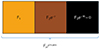Fig. 1. Three-cell star occulted by a planet and its atmosphere.

We then have the out-of-transit spectrum given by

$$\begin{array}{c}\hfill {\mathrm{F}}_{\mathrm{out}}(\lambda )={\mathrm{F}}_1(\lambda )+{\mathrm{F}}_2(\lambda )+{\mathrm{F}}_3(\lambda )\end{array}$$(1)

and the in-transit spectrum given by

$$\begin{array}{c}\hfill {\mathrm{F}}_{\mathrm{in}}^{\mathrm{pl}+\mathrm{atm}}(\lambda )={\mathrm{F}}_1(\lambda )+{\mathrm{F}}_2(\lambda )\times {\mathrm{e}}^{-\tau (\lambda )},\end{array}$$(2)

where F_i is the local flux coming from the stellar cells, λ is the wavelength dependence, and e( − τ) shows that during the transit F₂ has been absorbed by the planetary atmosphere, with τ the optical depth of the atmosphere. The absorption spectrum is given by

$$\begin{array}{c}\hfill {\mathcal{A}}_{\mathrm{pl}+\mathrm{atm}}(\lambda )=\frac{{\mathrm{F}}_{\mathrm{out}}(\lambda )-{\mathrm{F}}_{\mathrm{in}}^{\mathrm{pl}+\mathrm{atm}}(\lambda )}{{\mathrm{F}}_{\mathrm{out}}(\lambda )}=\frac{{\mathrm{F}}_2(\lambda )\times (1-{\mathrm{e}}^{-\tau (\lambda )})+{\mathrm{F}}_3(\lambda )}{{\mathrm{F}}_1(\lambda )+{\mathrm{F}}_2(\lambda )+{\mathrm{F}}_3(\lambda )}·\end{array}$$(3)

In the following equations we have dropped the wavelength dependence subscript for clarity.

In the literature, it is common to simulate the absorption spectrum using only the opaque planetary body. The observed absorption spectrum is then divided by this simulated absorption spectrum to correct for the POLDs and supposedly derive the absorption spectrum of the planetary atmosphere. The residual is often fitted, and atmospheric properties are then derived from this signal. The simulated absorption spectrum of the opaque planetary body, in our example, can be written as

$$\begin{array}{c}\hfill {\mathcal{A}}_{\mathrm{pl}}=\frac{{\mathrm{F}}_{\mathrm{out}}-{\mathrm{F}}_{\mathrm{in}}^{\mathrm{pl}}}{{\mathrm{F}}_{\mathrm{out}}}=\frac{{\mathrm{F}}_3}{{\mathrm{F}}_1+{\mathrm{F}}_2+{\mathrm{F}}_3}·\end{array}$$(4)

Dividing Eq. (3) by Eq. (4), we get

$$\begin{array}{cc}\hfill \frac{{\mathcal{A}}_{\mathrm{pl}+\mathrm{atm}}}{{\mathcal{A}}_{\mathrm{pl}}}& =\frac{{\mathrm{F}}_2\times (1-e^{-\tau })+{\mathrm{F}}_3}{{\mathrm{F}}_3}\hfill \\ \hfill & =1+(1-e^{-\tau })\frac{{\mathrm{F}}_2}{{\mathrm{F}}_3}·\hfill \end{array}$$(5)

After this supposed correction, a factor F₂/F₃ still affects the atmospheric signature, e^−τ.

2.2. Generalisation to a discretised stellar disc

In this section we generalise the derivation described above to a number of stellar cells, n. The out-of-transit spectrum is given by

$$\begin{array}{c}\hfill {\displaystyle {\mathrm{F}}_{\mathrm{out}}={\displaystyle \sum _{i=1}^n}{\mathrm{F}}_i,}\end{array}$$(6)

where the i index runs over all the cells of the stellar disc. The in-transit spectrum is given by

$$\begin{array}{c}\hfill {\displaystyle {\mathrm{F}}_{\mathrm{in}}^{\mathrm{pl}+\mathrm{atm}}={\displaystyle \sum _{i=1}^n}{\mathrm{F}}_i{e}^{-{\tau }_i},}\end{array}$$(7)

with τ_i the spectral optical depth of the atmospheric column occulting the stellar cell, i. It is equal to 0 (e^−τ_i = 1) when there is no atmosphere or planetary opaque body in front of the stellar cell, i. It tends to infinity (e^−τ_i = 0) for all wavelengths when the cell is behind the planetary disc. It also tends to infinity for specific wavelengths when the cell is behind a part of the atmosphere that is optically thick.

The absorption spectrum from the planet and the atmosphere is given as

$$\begin{array}{c}\hfill {\mathcal{A}}_{\mathrm{pl}+\mathrm{atm}}=\frac{\stackrel{{\mathrm{F}}_{\mathrm{abs}\mathrm{pl}}}{\overbrace{{\displaystyle \sum _k^K{\mathrm{F}}_k}}}+\stackrel{{\mathrm{F}}_{\mathrm{abs}\mathrm{atm}}}{\overbrace{{\displaystyle \sum _l^L{\mathrm{F}}_l(1-e^{-{\tau }_l})}}}}{{\displaystyle \sum _{\mathrm{i}=1}^{\mathrm{n}}{\mathrm{F}}_{\mathrm{i}}}},\end{array}$$(8)

where the k index runs over the stellar cells that are occulted by the planetary opaque disc at a specific timestep, and the l index runs over the stellar cells occulted by the planetary atmosphere at a specific timestep. The absorption spectrum by the opaque planetary body is given by

$$\begin{array}{c}\hfill {\mathcal{A}}_{\mathrm{pl}}=\frac{\stackrel{{\mathrm{F}}_{\mathrm{abs}\mathrm{pl}}}{\overbrace{{\displaystyle \sum _k^K{\mathrm{F}}_k}}}}{{\displaystyle \sum _{\mathrm{i}=1}^{\mathrm{n}}{\mathrm{F}}_{\mathrm{i}}}}·\end{array}$$(9)

Dividing Eq. (8) by Eq. (9) to isolate the absorption spectrum of the atmosphere, we get

$$\begin{array}{cc}\hfill \frac{{\mathcal{A}}_{\mathrm{pl}+\mathrm{atm}}}{{\mathcal{A}}_{\mathrm{pl}}}& =\frac{{\displaystyle \sum _k^K{\mathrm{F}}_k+{\displaystyle \sum _l^L}{\mathrm{F}}_l(1-e^{-{\tau }_l})}}{{\displaystyle \sum _k^K{\mathrm{F}}_k}}\hfill \\ \hfill & =1+\frac{{\displaystyle \sum _l^L{\mathrm{F}}_l(1-e^{-{\tau }_l})}}{{\displaystyle \sum _k^K{\mathrm{F}}_k}}·\hfill \end{array}$$(10)

Under the assumption of an atmosphere with a constant optical depth surrounding the planet, the equation becomes

$$\begin{array}{cc}\hfill \frac{{\mathcal{A}}_{\mathrm{pl}+\mathrm{atm}}}{{\mathcal{A}}_{\mathrm{pl}}}& =1+(1-e^{-\tau })\frac{{\displaystyle \sum _l^L{\mathrm{F}}_l}}{{\displaystyle \sum _k^K{\mathrm{F}}_k}}·\hfill \end{array}$$(11)

This means that the true atmospheric absorption signature is modulated by the ratio of the flux occulted by the atmosphere and the flux occulted by the planet. With centre-to-limb variation, stellar rotation, and other phenomena, inducing local variation in the stellar spectrum over the surface of the star, the flux behind the planet is expected to differ from the flux behind the atmosphere, especially for broad atmospheres and large planets. Therefore, one can expect the flux ratio to deform the true atmospheric absorption signature.

If we consider the flux to be constant over the whole stellar surface, then Eq. (11) becomes

$$\begin{array}{c}\hfill \frac{{\mathcal{A}}_{\mathrm{pl}+\mathrm{atm}}}{{\mathcal{A}}_{\mathrm{pl}}}=1+(1-e^{-\tau })\frac{{\mathrm{S}}_{\mathrm{atm}}}{{\mathrm{S}}_{\mathrm{pl}}},\end{array}$$(12)

with S_pl and S_atm being the projected surface of the opaque apparent planetary disc and the projected surface of the atmospheric annulus, respectively.

However, in the case with constant flux over the stellar surface and constant planetary atmospheric optical depth, the absorption spectrum, Eq. (8)¹, becomes

$$\begin{array}{c}\hfill {\mathcal{A}}_{\mathrm{pl}+\mathrm{atm}}=\frac{{\mathrm{S}}_{\mathrm{pl}}+{\mathrm{S}}_{\mathrm{atm}}(1-{\mathrm{e}}^{-\tau })}{{\mathrm{S}}_{\ast }},\end{array}$$(13)

where S_* is the projected surface of the apparent stellar disc. To make it equivalent to Eq. (12) and keep the same line-to-continuum ratio, one can multiply Eq. (13) by the surface ratio of the star to the planet:

$$\begin{array}{c}\hfill {\mathcal{A}}_{\mathrm{pl}+\mathrm{atm}}\times \frac{{\mathrm{S}}_{\ast }}{{\mathrm{S}}_{\mathrm{pl}}}=1+(1-{\mathrm{e}}^{-\tau })\frac{{\mathrm{S}}_{\mathrm{atm}}}{{\mathrm{S}}_{\mathrm{pl}}}=\frac{{\mathcal{A}}_{\mathrm{pl}+\mathrm{atm}}}{{\mathcal{A}}_{\mathrm{pl}}}·\end{array}$$(14)

A more formal expression for the bias, ℬ_𝒜, can be given by the difference between Eqs. (10) and (14),

$$\begin{array}{cc}\hfill {\mathcal{B}}_{\mathcal{A}}& \equiv \frac{{\mathcal{A}}_{\mathrm{pl}+\mathrm{atm}}}{{\mathcal{A}}_{\mathrm{pl}}}-{\frac{{\mathcal{A}}_{\mathrm{pl}+\mathrm{atm}}}{{\mathcal{A}}_{\mathrm{pl}}}|}_{\mathrm{sim}}\hfill \\ \hfill & =\frac{{\displaystyle \sum _l^L{\mathrm{F}}_l(1-e^{-{\tau }_l})}}{{\displaystyle \sum _k^K{\mathrm{F}}_k}}-{\displaystyle \sum _l^L}(1-e^{-{\tau }_l})\frac{{\mathrm{S}}_l}{{\mathrm{S}}_{\mathrm{pl}}}\hfill \\ \hfill & ={\displaystyle \sum _l^L}(1-e^{-{\tau }_l})[\frac{{\mathrm{F}}_l}{{\mathrm{F}}_{\mathrm{pl}}}-\frac{{\mathrm{S}}_l}{{\mathrm{S}}_{\mathrm{pl}}}],\hfill \end{array}$$(15)

where the optical depth in Eq. (14) was included back in the sum, ${\displaystyle \sum _{\mathrm{k}}^{\mathrm{K}}{\mathrm{F}}_{\mathrm{k}}={\mathrm{F}}_{\mathrm{pl}}}$ and ${\displaystyle \sum _l^{\mathrm{L}}{\mathrm{S}}_l={\mathrm{S}}_{\mathrm{atm}}}$. The ‘sim’ subscript refers to the simplified form of the equation (Eq. (12)) when considering uniform stellar spectra and a constant atmospheric optical depth. If we use the setup from Fig. 1, we can write the bias as

$$\begin{array}{cc}\hfill {\mathcal{B}}_{\mathcal{A}}& =(1-e^{-\tau })[\frac{{\mathrm{F}}_{\mathrm{atm}}}{{\mathrm{F}}_{\mathrm{pl}}}-\frac{{\mathrm{S}}_{\mathrm{atm}}}{{\mathrm{S}}_{\mathrm{pl}}}]=(1-e^{-\tau })[\frac{{\mathrm{F}}_{\mathrm{atm}}}{{\mathrm{F}}_{\mathrm{pl}}}-\frac{{\mathrm{R}}_{\mathrm{atm}}^2-{\mathrm{R}}_{\mathrm{pl}}^2}{{\mathrm{R}}_{\mathrm{pl}}^2}]\hfill \\ \hfill & =(1-e^{-\tau })[\frac{{\mathrm{F}}_{\mathrm{atm}}}{{\mathrm{F}}_{\mathrm{pl}}}-({\alpha }^2-1)]\hfill \end{array}$$(16)

if we assume R_atm = αR_pl, with α > 1, F₂ = F_atm, and F₃ = F_pl.

3. Estimates of the residual biases: A simplified framework

In this section we use transit simulations of a simplified planetary system setup to illustrate the possible biases to be expected on the derived planetary atmosphere parameters when correcting transit absorption spectra via division.

3.1. The star

We simulated the star as a disc discretised by a two-dimensional square grid that we filled with synthetic spectra, accounting for centre-to-limb variations of the lines’ profiles, broadband limb darkening, and stellar rotation. To simulate the synthetic spectra, we used the non-local thermodynamic equilibrium version of the Turbospectrum code for spectral synthesis (Alvarez & Plez 1998; Plez 2012; Heiter et al. 2021; Larsen et al. 2022; Magg et al. 2022), along with a MARCS photospheric model (Gustafsson et al. 2008) for the temperature, log g, and metallicity of the star HD 209458 (see Table 1), the host star of a well-known exoplanet (Henry et al. 2000; Charbonneau et al. 2000), and line lists from the VALD3 database (Ryabchikova et al. 2015). We restricted ourselves to a wavelength region around the sodium doublet in the visible to study the impact on a typical atmospheric sodium signature in a transiting close-in exoplanet.

3.2. The transiting planet and atmosphere

We studied 12 different cases for which we varied the position of the planet, the size of the atmosphere, and the v_eqsin(i) of the star². Table 2 shows the values that we used in the simulations for a specific atmosphere size. We used two sizes: an atmospheric radius of 1.5 times or 2 times the planetary radius of HD 209458 b, which is about 0.1145 times the radius of HD 209458. Once the spectra were distributed on the stellar grid, the out-of-transit spectrum was computed by summing the spectra from all the cells. To generate the in-transit spectra, we set the spectra from stellar cells behind the planet to zero and multiplied the spectra from the stellar cells behind the planetary atmosphere by e^−τ before computing the sum. For simplicity, we considered a homogeneous optical depth, τ, for the whole atmosphere. The optical depth³ is defined as

$$\begin{array}{c}\hfill \tau (\lambda )=\frac{\pi e^2}{m_{e}c}{f}_{\mathrm{osc}}\varphi (\lambda -{\lambda }_0,w)n_{\mathrm{col}},\end{array}$$(17)

with ϕ(λ − λ₀, w) the line profile (we used a Voigt profile in this study), n_col the column density, ${\displaystyle \mathit{w}=\sqrt{\frac{2k_{b}T}{m}}}$ the thermal broadening, T the temperature of sodium atoms, f_osc the oscillator strength of the transition, k_b the Boltzmann constant, m the mass of a sodium atom, e the electron electric charge, m_e its mass, and c the speed of light; λ₀ is the wavelength of reference for the atomic transitions of interest, here the Na I D2 line. No velocity field was included in the atmosphere. In the following simulations the temperature of the atmosphere was set to 10 000 K and the column density was set to 7 × 10¹¹ at. cm⁻². This allowed us to produce a sodium atmospheric absorption signature of about 0.6 and 1.4% for the case with R_atm = 1.5 R_pl and R_atm = 2.0 R_pl, respectively (see the black curves in Figs. 2 and 3).

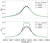Fig. 2. Comparison of the corrected absorption spectrum (Eq. (10)) and the pure absorption signature (Eq. (14)) for an atmosphere with a radius of 1.5 times the planetary radius. Upper panel: When the planet is at x, y = ( − 0.5; 0). Lower panel: When the planet is at x, y = (0; 0), the centre of the stellar disc.

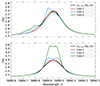Fig. 3. Comparison of the corrected absorption spectrum (Eq. (10)) and the pure absorption signature (Eq. (14)) for an atmosphere with a radius of 2.0 times the planetary radius. Upper panel: When the planet is at x, y = ( − 0.5; 0). Lower panel: When the planet is at x, y = (0; 0), the centre of the stellar disc.

3.3. Results of the simulations

Figures 2 and 3 show the results of the simulations for the six different cases for an atmosphere of radius 1.5 times the planetary radius and 2.0 times the planetary radius, respectively. It is clear that when centre-to-limb variations and stellar rotation are included in the stellar spectrum, the result of Eq. (10) diverges from the unaffected absorption spectrum of the atmosphere (Eq. (14)). With a line profile that varies, one can expect the derived values for the atmosphere’s properties to be biased. Moreover, the line profile sometimes appears to have a shifted component (e.g. case 4 with a planet position not at the centre of the star), which could be wrongly interpreted as winds in the atmosphere when there are none. This means that correcting the absorption spectrum with the synthetic absorption spectrum of the planetary opaque body is not a reliable method.

The goal of dividing the absorption spectrum by the synthetic absorption spectrum of the planet is to correct for the POLDs and thus extract an unaffected absorption spectrum for the planetary atmosphere (Eq. (14)). Therefore, in order to estimate the bias left by the division on the true atmospheric signature, we used Eq. (14) to fit the result of Eq. (10). Here, only the temperature and the column density are free parameters. We used a simple least square algorithm for the fit. Table 3 shows the errors on the temperature and column density for the six cases for an atmosphere with a radius of 1.5 and 2.0 times the planetary radius. The values of the errors should only serve to demonstrate that resorting to division by the absorption spectrum of the planetary body to extract the atmospheric signal will lead to wrong estimates of the true properties of the planetary atmosphere.

4. Conclusion

We have demonstrated that correcting absorption spectra via division by a simulated absorption spectrum of a bare planet does not allow one to extract the pure atmospheric signal. Only in the most idealistic case (i.e. uniform stellar spectra and a constant atmospheric optical depth) can one hope to derive unbiased properties. In addition, we have shown how the atmospheric signal can be distorted when centre-to-limb variations in line profiles and stellar rotation are included in the stellar spectrum. We have shown that in the case of a typical Jupiter-sized planet with a typical sodium atmospheric signal, the retrieved properties of the atmosphere can significantly differ from the true value. Stellar rotation being one of the dominant effects that modify local spectra, the bias left after the correction is more significant with increasing v_eqsin(i).

These results are particularly crucial for studies of planetary atmospheric escape. Under hydrodynamic escape, an atmosphere can occupy a broad and sometimes asymmetric region (i.e. with escaping tails and bow shocks) around the planet (e.g. Bourrier et al. 2015, 2018; Carolan et al. 2021; Spake et al. 2021; Tyler et al. 2024; Gully-Santiago et al. 2024), leading the planet and the atmosphere to absorb very different spectra. One can thus expect the atmospheric signature to be distorted in the absorption spectrum if it is corrected with a simulated absorption spectrum of the bare planet. It is, however, worth noting that atmospheric escape studies are usually done on hydrogen and helium lines. The exact behaviour of such lines with respect to centre-to-limb variations might be different from that of the Na I doublet lines. Therefore, the impact of the problematic identified in this study might differ and would be worth investigating.

On the contrary, the residual biases after the correction, although present, might become negligible when studying transit observations of Earth-sized planets. With a smaller size, the spectra absorbed by the opaque body and the atmosphere could be similar enough for the flux ratio (identified in Eq. (15)) to be close to 1, potentially lessening the challenge of characterising these planets.

This study was conducted with synthetic spectra, and the exact absorption spectrum of the planetary opaque body was used for the corrections of the absorption spectra. We have thus mitigated the impact of the correction on the residual atmospheric signal. However, with observations, the noise and the instrumental response can further affect the true atmospheric signal, and one might not simulate the exact absorption spectrum of the planet for the correction, which would lead to a possibly unforeseen bias. Moreover, all the simulations were performed with absolute flux spectra. This means there was no need for normalisation. As pointed out by Dethier & Bourrier (2023), normalisation can affect the amplitude of the atmospheric absorption signature. Therefore, with non-flux-calibrated transit observations that, thus, require normalisation, the derived absorption signature after correction might be modified even more strongly than without normalisation, potentially leading to even more divergent results.

Finally, in this work we decided to use absorption spectra to demonstrate our argument that a bias is left after the correction. However, this argument still holds when using transmission spectra. The equations given here would need to be adapted (see Appendix A), and the exact residual bias would change but would still be present. A detailed description of how the bias behaves when correcting absorption and transmission spectra would require an in-depth study that explores the parameters affecting the spectra contained in Eq. (10) (e.g. stellar rotation, planetary and atmosphere size, spectral type, specific lines, etc.), which is not the intent of this study.

The method of correcting the high-resolution absorption spectrum of a transiting planet using a simulated absorption spectrum of the bare planet is, therefore, not a sustainable method for extracting unbiased properties of a transiting exoplanet atmosphere. We therefore advise using a different approach, one in which both a planet and an atmosphere are simulated during the transit to derive a self-consistent absorption spectrum (e.g. Dethier & Bourrier 2023). In this way, the simulated absorption spectra can be directly compared to the absorption spectra reconstructed from observations without further corrections.

Acknowledgments

The author greatly thanks the referee for their relevant suggestions that allowed us to improve our study. Funded/Co-funded by the European Union (ERC, FIERCE, 101052347). Views and opinions expressed are however those of the author(s) only and do not necessarily reflect those of the European Union or the European Research Council. Neither the European Union nor the granting authority can be held responsible for them. This work was supported by FCT - Fundação para a Ciência e a Tecnologia through national funds and by these grants: UIDB/04434/2020; UIDP/04434/2020. This work has made use of the VALD database, operated at Uppsala University, the Institute of Astronomy RAS in Moscow, and the University of Vienna.

References

Appendix A: Equations of Sect 2.2 for transmission spectra

We remind the reader that, even though a transmission spectrum is defined as 𝒯 = 1 − 𝒜, the corrected transmission spectrum is not equal to 1 minus the corrected absorption spectrum. Rather, it is equal to ${\mathcal{T}}_{\mathrm{corr}}=\frac{{\mathcal{T}}_{\mathrm{pl}+\mathrm{atm}}}{{\mathcal{T}}_{\mathrm{pl}}}=\frac{1-{\mathcal{A}}_{\mathrm{pl}+\mathrm{atm}}}{1-{\mathcal{A}}_{\mathrm{pl}}}$.

As such, the equations provided in the main document for the absorption spectra cannot simply be transformed using 1 minus a given equation for the absorption spectrum. Below, we give the equivalent of Eqs. 8 to 14 from Sect. 2.2 in the case of transmission spectra instead of absorption spectra.

The transmission spectrum of the planet and its atmosphere is written as

$$\begin{array}{c}\hfill {\mathcal{T}}_{\mathrm{pl}+\mathrm{atm}}=\frac{\stackrel{{\mathrm{F}}_{\mathrm{unocc}}}{\overbrace{{\displaystyle \sum _j^J{\mathrm{F}}_j}}}+\stackrel{{\mathrm{F}}_{\mathrm{trans}\mathrm{atm}}}{\overbrace{{\displaystyle \sum _l^L{\mathrm{F}}_l{e}^{-{\tau }_l}}}}}{{\displaystyle \sum _{\mathrm{i}=1}^{\mathrm{n}}{\mathrm{F}}_{\mathrm{i}}}},\end{array}$$(A.1)

where the j index runs on the cells that are not occulted, neither by the planet nor the atmosphere. F_{trans atm} designates the flux transmitted through the atmosphere.

The transmission spectrum of the planet is written as

$$\begin{array}{c}\hfill {\mathcal{T}}_{\mathrm{pl}}=\frac{\stackrel{{\mathrm{F}}_{\mathrm{unocc}}}{\overbrace{{\displaystyle \sum _j^J{\mathrm{F}}_j}}}+\stackrel{{\mathrm{F}}_{\mathrm{unocc}\mathrm{atm}}}{\overbrace{{\displaystyle \sum _l^L{\mathrm{F}}_l}}}}{{\displaystyle \sum _{\mathrm{i}=1}^{\mathrm{n}}{\mathrm{F}}_{\mathrm{i}}}},\end{array}$$(A.2)

where F_{unocc atm} designates the flux behind the atmospheric annulus. The corrected transmission spectrum is written as

$$\begin{array}{c}\hfill \frac{{\mathcal{T}}_{\mathrm{pl}+\mathrm{atm}}}{{\mathcal{T}}_{\mathrm{pl}}}=\frac{{\displaystyle \sum _j^J{\mathrm{F}}_j+{\displaystyle \sum _l^L}{\mathrm{F}}_l{e}^{-{\tau }_l}}}{{\displaystyle \sum _j^J{\mathrm{F}}_j+{\displaystyle \sum _l^L}{\mathrm{F}}_l}}.\end{array}$$(A.3)

Under the assumptions of uniform stellar spectra and a constant atmospheric optical depth, we simplify Eq. A.3 as

$$\begin{array}{cc}\hfill \frac{{\mathcal{T}}_{\mathrm{pl}+\mathrm{atm}}}{{\mathcal{T}}_{\mathrm{pl}}}=& \frac{{\mathrm{S}}_{\ast }-{\mathrm{S}}_{\mathrm{pl}}-{\mathrm{S}}_{\mathrm{atm}}+{\mathrm{S}}_{\mathrm{atm}}{\mathrm{e}}^{-\tau }}{{\mathrm{S}}_{\ast }-{\mathrm{S}}_{\mathrm{pl}}}\hfill \\ \hfill =& 1+(e^{-\tau }-1)\frac{{\mathrm{S}}_{\mathrm{atm}}}{{\mathrm{S}}_{\ast }-{\mathrm{S}}_{\mathrm{pl}}}.\hfill \end{array}$$(A.4)

Under the same assumptions, Eq. A.1 is written as

$$\begin{array}{c}\hfill {\mathcal{T}}_{\mathrm{pl}+\mathrm{atm}}=\frac{{\mathrm{S}}_{\ast }-{\mathrm{S}}_{\mathrm{pl}}+{\mathrm{S}}_{\mathrm{atm}}({\mathrm{e}}^{-\tau }-1)}{{\mathrm{S}}_{\ast }},\end{array}$$(A.5)

which becomes equivalent to Eq. A.4 after the following operation,

$$\begin{array}{c}\hfill {\mathcal{T}}_{\mathrm{pl}+\mathrm{atm}}\times \frac{{\mathrm{S}}_{\ast }}{{\mathrm{S}}_{\ast }-{\mathrm{S}}_{\mathrm{pl}}}=1+({\mathrm{e}}^{-\tau }-1)\frac{{\mathrm{S}}_{\mathrm{atm}}}{{\mathrm{S}}_{\ast }-{\mathrm{S}}_{\mathrm{pl}}}.\end{array}$$(A.6)

Finally, the bias is defined as Eq. A.3 minus Eq. A.6,

$$\begin{array}{cc}\hfill {\mathcal{B}}_{\mathcal{T}}& \equiv \frac{{\mathcal{T}}_{\mathrm{pl}+\mathrm{atm}}}{{\mathcal{T}}_{\mathrm{pl}}}-{\frac{{\mathcal{T}}_{\mathrm{pl}+\mathrm{atm}}}{{\mathcal{T}}_{\mathrm{pl}}}|}_{\mathrm{sim}}\hfill \\ \hfill & =\frac{{\displaystyle \sum _j^J{\mathrm{F}}_j+{\displaystyle \sum _l^L}{\mathrm{F}}_l{e}^{-{\tau }_l}}}{{\displaystyle \sum _j^J{\mathrm{F}}_j+{\displaystyle \sum _l^L}{\mathrm{F}}_l}}-1-\frac{{\displaystyle \sum _l^L(e^{-{\tau }_l}-1){\mathrm{S}}_l}}{{\mathrm{S}}_{\ast }-{\mathrm{S}}_{\mathrm{pl}}}\hfill \\ \hfill & =\frac{{\displaystyle {\mathrm{F}}_{\ast }-{\mathrm{F}}_{\mathrm{pl}}-{\mathrm{F}}_{\mathrm{atm}}+{\displaystyle \sum _l^{\mathrm{L}}}{\mathrm{F}}_l{\mathrm{e}}^{-{\tau }_l}}}{{\mathrm{F}}_{\ast }-{\mathrm{F}}_{\mathrm{pl}}}-1-\frac{{\displaystyle \sum _l^L(e^{-{\tau }_l}-1){\mathrm{S}}_l}}{{\mathrm{S}}_{\ast }-{\mathrm{S}}_{\mathrm{pl}}}\hfill \\ \hfill & =\frac{{\displaystyle \sum _l^{\mathrm{L}}{\mathrm{F}}_l{\mathrm{e}}^{-{\tau }_l}-F_{\mathrm{atm}}}}{{\mathrm{F}}_{\ast }-{\mathrm{F}}_{\mathrm{pl}}}-\frac{{\displaystyle \sum _l^L(e^{-{\tau }_l}-1){\mathrm{S}}_l}}{{\mathrm{S}}_{\ast }-{\mathrm{S}}_{\mathrm{pl}}}\hfill \\ \hfill & =\frac{{\displaystyle \sum _l^{\mathrm{L}}{\mathrm{F}}_l({\mathrm{e}}^{-{\tau }_l}-1)}}{{\mathrm{F}}_{\ast }-{\mathrm{F}}_{\mathrm{pl}}}-\frac{{\displaystyle \sum _l^L(e^{-{\tau }_l}-1){\mathrm{S}}_l}}{{\mathrm{S}}_{\ast }-{\mathrm{S}}_{\mathrm{pl}}}\hfill \\ \hfill & ={\displaystyle \sum _l^{\mathrm{L}}({\mathrm{e}}^{-{\tau }_l}-1)}[\frac{{\mathrm{F}}_l}{{\mathrm{F}}_{\ast }-{\mathrm{F}}_{\mathrm{pl}}}-\frac{{\mathrm{S}}_l}{{\mathrm{S}}_{\ast }-{\mathrm{S}}_{\mathrm{pl}}}].\hfill \end{array}$$(A.7)

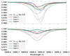Fig. A.1. Comparison of the corrected transmission spectrum (Eq. A.3) and the pure transmission signature (Eq. A.6) for an atmosphere with a radius of 1.5 times the planetary radius (plain curves) and 2.0 times the planetary radius (dotted curves). Upper panel: When the planet is at x, y = ( − 0.5; 0). Lower panel: When the planet is at x, y = (0; 0), the centre of the stellar disc.

All Tables

All Figures

	Fig. 1. Three-cell star occulted by a planet and its atmosphere.
In the text

	Fig. 2. Comparison of the corrected absorption spectrum (Eq. (10)) and the pure absorption signature (Eq. (14)) for an atmosphere with a radius of 1.5 times the planetary radius. Upper panel: When the planet is at x, y = ( − 0.5; 0). Lower panel: When the planet is at x, y = (0; 0), the centre of the stellar disc.
In the text

	Fig. 3. Comparison of the corrected absorption spectrum (Eq. (10)) and the pure absorption signature (Eq. (14)) for an atmosphere with a radius of 2.0 times the planetary radius. Upper panel: When the planet is at x, y = ( − 0.5; 0). Lower panel: When the planet is at x, y = (0; 0), the centre of the stellar disc.
In the text

	Fig. A.1. Comparison of the corrected transmission spectrum (Eq. A.3) and the pure transmission signature (Eq. A.6) for an atmosphere with a radius of 1.5 times the planetary radius (plain curves) and 2.0 times the planetary radius (dotted curves). Upper panel: When the planet is at x, y = ( − 0.5; 0). Lower panel: When the planet is at x, y = (0; 0), the centre of the stellar disc.
In the text

References

- Alvarez, R., & Plez, B. 1998, A&A, 330, 1109 [NASA ADS] [Google Scholar]
- Bourrier, V., Ehrenreich, D., & Lecavelier des Etangs, A. 2015, A&A, 582, A65 [NASA ADS] [CrossRef] [EDP Sciences] [Google Scholar]
- Bourrier, V., Lecavelier des Etangs, A., Ehrenreich, D., et al. 2018, A&A, 620, A147 [NASA ADS] [CrossRef] [EDP Sciences] [Google Scholar]
- Carolan, S., Vidotto, A. A., Hazra, G., Villarreal D’Angelo, C., & Kubyshkina, D. 2021, MNRAS, 508, 6001 [NASA ADS] [CrossRef] [Google Scholar]
- Casasayas-Barris, N., Palle, E., Nowak, G., et al. 2017, A&A, 608, A135 [NASA ADS] [CrossRef] [EDP Sciences] [Google Scholar]
- Casasayas-Barris, N., Pallé, E., Yan, F., et al. 2018, A&A, 616, A151 [NASA ADS] [CrossRef] [EDP Sciences] [Google Scholar]
- Casasayas-Barris, N., Pallé, E., Yan, F., et al. 2020, A&A, 635, A206 [NASA ADS] [CrossRef] [EDP Sciences] [Google Scholar]
- Charbonneau, D., Brown, T. M., Latham, D. W., & Mayor, M. 2000, ApJ, 529, L45 [Google Scholar]
- Dethier, W., & Bourrier, V. 2023, A&A, 674, A86 [NASA ADS] [CrossRef] [EDP Sciences] [Google Scholar]
- Gully-Santiago, M., Morley, C. V., Luna, J., et al. 2024, AJ, 167, 142 [NASA ADS] [CrossRef] [Google Scholar]
- Gustafsson, B., Edvardsson, B., Eriksson, K., et al. 2008, A&A, 486, 951 [NASA ADS] [CrossRef] [EDP Sciences] [Google Scholar]
- Heiter, U., Lind, K., Bergemann, M., et al. 2021, A&A, 645, A106 [EDP Sciences] [Google Scholar]
- Henry, G. W., Marcy, G. W., Butler, R. P., & Vogt, S. S. 2000, ApJ, 529, L41 [Google Scholar]
- Keles, E., Czesla, S., Poppenhaeger, K., et al. 2024, MNRAS, 530, 4826 [NASA ADS] [CrossRef] [Google Scholar]
- Larsen, S. S., Eitner, P., Magg, E., et al. 2022, A&A, 660, A88 [NASA ADS] [CrossRef] [EDP Sciences] [Google Scholar]
- Magg, E., Bergemann, M., Serenelli, A., et al. 2022, A&A, 661, A140 [NASA ADS] [CrossRef] [EDP Sciences] [Google Scholar]
- Maguire, C., Gibson, N. P., Nugroho, S. K., et al. 2023, MNRAS, 519, 1030 [Google Scholar]
- Maguire, C., Gibson, N. P., Nugroho, S. K., et al. 2024, A&A, 687, A49 [NASA ADS] [CrossRef] [EDP Sciences] [Google Scholar]
- Masson, A., Vinatier, S., Bézard, B., et al. 2024, A&A, 688, A179 [NASA ADS] [CrossRef] [EDP Sciences] [Google Scholar]
- Nugroho, S. K., Gibson, N. P., de Mooij, E. J. W., et al. 2020, MNRAS, 496, 504 [Google Scholar]
- Plez, B. 2012, Astrophysics Source Code Library [record ascl:1205.004] [Google Scholar]
- Ryabchikova, T., Piskunov, N., Kurucz, R. L., et al. 2015, Phys. Scr., 90, 054005 [Google Scholar]
- Spake, J. J., Oklopčić, A., & Hillenbrand, L. A. 2021, AJ, 162, 284 [NASA ADS] [CrossRef] [Google Scholar]
- Tyler, D., Petigura, E. A., Oklopčić, A., & David, T. J. 2024, ApJ, 960, 123 [NASA ADS] [CrossRef] [Google Scholar]
- Yan, F., & Henning, T. 2018, Nat. Astron., 2, 714 [Google Scholar]