| Issue |
A&A
Volume 688, August 2024
|
|
|---|---|---|
| Article Number | A70 | |
| Number of page(s) | 17 | |
| Section | Interstellar and circumstellar matter | |
| DOI | https://doi.org/10.1051/0004-6361/202347529 | |
| Published online | 06 August 2024 | |
Scattering properties of protoplanetary dust analogs with microwave analogy: Rough compact grains
1
Aix Marseille Univ, CNRS, Centrale Med, Institut Fresnel,
Marseille,
France
e-mail: This email address is being protected from spambots. You need JavaScript enabled to view it.
2
Univ. Grenoble Alpes, CNRS, IPAG,
38000
Grenoble,
France
3
LPC2E, Université d’Orléans, CNRS,
Orléans,
France
Received:
21
July
2023
Accepted:
20
May
2024
Abstract
Context. Scattering simulations of perfect spheres are not sufficient to explain the observations of scattered light from protoplanetary and debris disks, especially when the dust sizes are on the same order of magnitude as the wavelength used to perform the observations. Moreover, examples of grains collected from the Solar System have proved that the morphology of interstellar dust is irregular. These pieces of evidence lead us to consider that the morphologies of the dust that participates in these circumstellar disks are more complex than those of spheres.
Aims. We aim to measure and simulate the scattering properties of six rough compact grains to identify how their morphology affects their scattering properties. These grains are intended to be dust analogs of protoplanetary and debris disks. Their convexity ranges from 75% to 99%.
Methods. Grains were 3D printed using stereolithography, and their shape and refractive index were controlled. These analogs were measured with our microwave-scattering experiment (microwave analogy) at wavelengths ranging from 16.7 mm to 100 mm, leading to size parameters from X = 1.07 to X = 7.73. In parallel, their scattering properties were simulated with our finite-element method (FEM), which contained the same geometric file as the 3D printed grains.
Results. We retrieved five scattering properties of these grains, that is, the phase function, the degree of linear polarization (DLP), and three other Mueller matrix elements 〈Sij〉. Two types of studies were performed. First, a study of the scattering properties averaged over several orientations of grains at different wavelengths. Second, a study of the same scattering properties, for which a power-law size distribution effect was applied.
Conclusions. The very good correspondence between the measured and simulated Mueller matrix elements demonstrated the accuracy of our measurement setup and the efficiency of our FEM simulations. For the first study, DLP proved to be a good indicator of the grain morphology in terms of convexity and shape anisotropy. For the second study, backscattering enhancements of the phase function were related to the grain convexity. The maximum DLP and its negative polarization branches as well as the 〈S22〉/〈S11〉 levels were related to the shape anisotropy of our grains.
Key words: polarization / scattering / comets: general / protoplanetary disks
© The Authors 2024
 Open Access article, published by EDP Sciences, under the terms of the Creative Commons Attribution License (https://creativecommons.org/licenses/by/4.0), which permits unrestricted use, distribution, and reproduction in any medium, provided the original work is properly cited.
This article is published in open access under the Subscribe to Open model. This email address is being protected from spambots. You need JavaScript enabled to view it. to support open access publication.
1 Introduction
In the context of planet formation, different disk stages are present, such as the protoplanetary disk and the debris disk, on which we focus here. Dust particles in protoplanetary disks undergo different growth processes that produce different outcomes, such as sticking, bouncing, fragmentation, abrasion, erosion, cratering, and mass transfer (Testi et al. 2014; Blum 2018). These outcomes affect the dust morphology and produce irregular grains. To proceed in understanding of this dust evolution, indirect information about their structure can be obtained with light-scattered observations of disks. The assumption that the dust is only composed of perfectly round spheres has been proved to be insufficient to align simulations and observations of the light that is scattered by protoplanetary dust (Kirchschlager & Bertrang 2020). Similarly, particles collected from asteroids and from the interstellar medium in the Solar System have demonstrated the presence of irregular interstellar dust particles. For example, recent samples collected by the Hayabusa 2 mission from the asteroid Ryugu revealed both rugged and smooth particles, providing information about the morphology of these primitive small Solar System bodies (Yada et al. 2022) and the dust that may eventually participate in the planet formation. Thus, dust particles with irregular shapes must be taken into account in the models, and the scattering properties of these structures must be studied.
For protoplanetary and debris disks, the commonly accepted dust size distribution is a power-law distribution of index -3.5 (Dohnanyi 1969; Draine 2006). For debris disks, this distribution results from an infinite cascade of collisions, while for protoplanetary disks, it results from different growth processes (grain-grain collision and condensation) that begin with interstellar particles of micron sizes (Mathis et al. 1977). For the two considered disks, the minimum dust size is about O.lµm to 10 µm (Mathis et al. 1977; Pawellek & Krivov 2015). The dust particles are sorted by their size parameter X = 2πR/λ, which is the ratio of the radius R of the smallest sphere bounding the particle and the wavelength λ used to perform the observation. For dust particles in the Rayleigh regime (X << 1), the light-scattering properties are well studied and easily computed (Bohren & Huffman 1983). For dust particles whose sizes are comparable to that of the wavelength, that is, at a size parameter X of about 1 or in the Mie scattering regime, the scattering properties become computationally demanding because the limits of what can be calculated in terms of time and memory consumption are reached. For large X size parameters, the advantage of having access to experiments is therefore fully realized. We focus on this particularly demanding range of size parameters, between X = 1.07 to X = 7.73, and aim to analyze the impact of the dust morphology on their scattering properties.
Previous studies have shown that the Lorentz-Mie solution for spheres was not appropriate to reproduce the scattering of irregular particles in the Mie regime. Hence, a series of experiments were launched to study the scattering properties of nonspherical structures by means of numerical simulations, light-scattering experiments, or microwave-scattering experiments. Mishchenko et al. (2000) summarized the main scattering properties of nonspherical particles that were reported in terms of the Mueller matrix elements 〈Sij〉, such as the phase function, the degree of linear polarization (DLP), or the circular depolarization. Table 1 provides a reference list of the size parameters and the refractive indexes of some of the scattering studies that have been published for rough particles.
Several numerical studies have simulated the scattering behaviors of virtual irregular particles created in different ways. For example, Liu et al. (2014); Zhang et al. (2016) generated virtual ice particles by taking a regular solid hexagon and altering its faces. Muinonen et al. (2007); Nousiainen & Muinonen (2007) constructed Gaussian random particles according to a given spatial covariance function. The particle scattering properties were numerically studied with the discrete dipole approximation method (DDA). Zubko et al. (2015) proposed an original type of virtual irregular particles (pocked spheres) for which DDA simulations were again used to study the scattering properties. Kahnert et al. (2011) performed scattering simulations with the T-matrix method for Chebyshev particles (based on Chebyshev polynomials) and compared them with measurements of hematite aerosol samples, without ascertaining that these samples indeed have a Chebyshev shape.
In numerical studies, several choices must be made, such as how the irregular particles are discretized, the level of mesh refinement, the roughness details that must be taken into account in the particle description, and the simulation algorithm. All these choices affect the simulated scattering properties and the analysis that is based on them. We opted for a 3D finite-element method (FEM) that solves the vectorial Helmholtz equation (Voznyuk et al. 2015) for a given orientation of the particle and a given illumination direction. The simulated scattered field is then transformed into the Jones matrix. Averaging in orientation and illumination, and using the transformation equations from Jones to Mueller elements (Bohren & Huffman 1983), leads to the Mueller matrix elements. The FEM method offers two main assets. First, it uses a conformal mesh, which ensures a faithful description of the particle surface roughness. Second, it requires solving a sparse linear system, which is less intensive computationally and in memory requirements than a dense matrix system as the particle size parameter increases.
For the sake of cross validation, it is also important to correlate the simulation with measurements. Numerical simulations must therefore be associated with laboratory scattering measurements, so that each approach complements the other and allows us to better understand the observations of protoplanetary and debris disks.
One way of obtaining the scattering properties of irregular particles is with light-scattering measurements. Escobar-Cerezo et al. (2017) studied the scattering properties of irregular cosmic dust analogs with laboratory measurements and ray-optics model simulations. Muñoz et al. (2020) measured the phase function and the DLP of cosmic dust analogs and compared them to the observed scattering properties of Comet 67P/Churyumov Gerasimenko. The size parameters of these two studies are in the geometrical scattering regime, however, which is not of interest here.
In order to be in the Mie scattering regime, microwave-scattering measurements are worth considering. The microwave analogy allows us to simultaneously generate irregular particles and observe them at a wavelength that is on the same order as the particle size. The microwave analogy is based on the scale invariance rule. This rule states that analog particles can have the same scattering properties as the real particles if the analog electromagnetic system has geometrical dimensions that are scaled in proportion to the incident wavelength while keeping the same refractive index (Mishchenko 2006). To respect this proportion, the size parameter (X) must remain the same.
Microwave-scattering measurements of irregular particles (spherical particles bounded by a rough surface and fluffy conglomerates) have been carried out since the 1980s (Mukai et al. 1982). Zerull (1985) measured two scattering properties, the phase function and the degree of linear polarization of several nonspherical particles in the microwave range, and compared them to the phase function and DLP of calculated Mie spheres. As expected, the discrepancy between the measurements and the simulations was clear, emphasizing the importance of properly addressing the issue related to the particle geometry. Furthermore, Zerull (1985) highlighted the advantages of the microwave range. In this frequency range, the orientation, size, shape, structure, and refractive index of the measured analogs can be controlled. Since then, these advantages have been enhanced because particle shape and size can now be controlled better, and a wider range of refractive indexes is accessible.
The aim of this work therefore is to study the scattering properties of six rough solid particles, called grains, which are intended to be analogs of protoplanetary and debris dust. To stay in the Mie regime, we performed the measurements in the microwave range at wavelengths ranging from λ = 16.7 mm to λ = 100 mm. The shape (roughness) and the refractive index of the particles were controlled with additive manufacturing processes that led to particles with a bounding radius ranging from 17 mm to 20.5 mm and a refractive index of m = 1.7 + 0.003i, which is close to the refractive index of the astronomical silicate (Draine & Lee 1984). The grains were also simulated numerically with our customized FEM method (Voznyuk et al. 2015), which is based on the same computer-aided design (CAD) file that was used to manufacture the analogs. Different scattering properties are studied: the phase function 〈S11〉 the degree of linear polarization (–〈S12〉/〈S11〉) and the other elements of the Mueller matrix (〈S22〉, 〈S34〉, and 〈S44〉), in order to understand how roughness and shape anisotropy may affect these scattering properties. This study is a continuation of our previous paper (Tobon Valencia et al. 2022), which studied the scattering properties of another morphology of protoplanetary dust analogs, that is, aggregates.
The paper is organized as follows. Section 2 describes the dust analog grains. Section 3 presents the scattering properties, as well as the way they were either measured or simulated. Section 4 discusses the results, and Sect. 5 details the conclusions and prospects for future works.
Some previous scattering studies of rough particles.
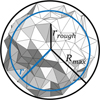 |
Fig. 1 Example of the virtual generation of our grains, where r is the initial radius of the sphere to mesh, rrough are the perturbed distances from the center of the sphere r to each triangle vertex, and Rmax is the radius of the bounding sphere, called maximum radius. |
2 Grain analogs
Dust particles in protoplanetary disks undergo different transformation processes that can lead to a wide range of possible morphologies. We focus on six different grains with varying roughness, each of which was derived from the same initial sphere. In order to produce them, two steps are necessary: they were generated virtually, and they were printed in 3D. This is described in the following subsections.
2.1 Virtual generation and 3D printing
All our grains were generated in the same way. First, a sphere of initial radius r = 16.25 mm was meshed with similar triangles. For all grains, the number of triangles was 320, except for the last object (Gr_n2_r13.2), for which it was set to 80. This provided a different roughness than its counterpart Gr_n2_r13.3. Afterward, the distance from the center of the sphere to the vertex of each triangle was perturbed with a random perturbation rrand, following a uniform distribution between −ls and +ls. This created a rough radius rrough (see Fig. 1, where Rmax is the radius of the bounding sphere of each grain after perturbation),
![Mathematical equation: ${r_{{\rm{rough }}}} = r + {r_{{\rm{rand }}}}\quad {r_{{\rm{rand }}}}\~{\cal U}\left( {\left[ { - {l_{\rm{s}}},1{\rm{s}}} \right]} \right),$](/articles/aa/full_html/2024/08/aa47529-23/aa47529-23-eq1.png) (1)
(1)
ls = λ/n was taken as the fraction of λ at λ = 30 mm, where the denominator n took values between 2 to 10. For the two roughest grains n = 2, this value increased with a step of 2 from n = 4 to n = 10 (this last value corresponds to the smoothest grain, close to a perfect sphere).
The grains were 3D printed with stereolithography, using acrylic resin with a refractive index of 1.7 + 0.03i, which is close to the refractive index of the astronomical silicate (Draine & Lee 1984). This same printing method and material were described and used in our previous paper (Tobon Valencia et al. 2022). Each grain is denoted by a technical name that is a string composed of Gr, which is the abbreviation of grain; n, which is the denominator of ls (see Eq. (1)), followed by its value; and then the letter r (roughness), followed by the percentage of the roughness of the grain (see Eq. (1)). Three of these grains were already presented in another collaborative study (Renard et al. 2021), but with different names: GravelLike corresponds to Gr_n2_r13.2, Rough sphere 223 corresponds to Gr_n2_r13.3, and Rough sphere 228 corresponds to Gr_n10_r2.6. Figure 2 shows the pictures of the printed grains with their corresponding technical name.
2.2 Morphology characterization
To characterize the grain morphology from its mesh file, we computed several quantities (Angelidakis et al. 2021), such as the shape anisotropy and the convexity. The inertia moments m1 ≥ m2 ≥ m3 enabled us to introduce three geometrical intrinsic quantities, such as the elongation, flatness, and shape anisotropy. They are defined as
 (2)
(2)
 (3)
(3)
 (4)
(4)
The closer to 100% these factors, the more spherical the grain. A small shape anisotropy factor indicates that the grain is elongated or flat in a particular direction. In the following, we therefore use this shape anisotropy as an indicator of the sphericity level of the grains.
The convexity is defined as
 (5)
(5)
where VCH corresponds to the volume of the convex hull associated with the grain. This indicator is tightly linked with the roughness of the grain when the convex hull shape is indeed close to a sphere. In this case, the closer to 100% the convexity, the more convex and thus roundish the grain surface. In the following, we therefore use this convexity as an indicator of the smoothness level of the grains.
Table 2 summarizes all the morphological properties of the grains, as well as the size parameter X = 2πRmax/λ, where the wavelength is provided at minimum and maximum values.
2.3 Grain size analogy
The mean radius Rmean of the bounding spheres of our six grains is 18.45 mm, leading to a mean size parameter Xmean = 2πRmean/λ ranging from Xmean = 1.16 to 6.94 (calculated based on Table 2). Assuming these same size parameters, the corresponding mean radius of protoplanetary dust would have different values, depending on the wavelength range chosen for the observations, as shown in Table 3.
3 Scattering properties
The electromagnetic fields scattered by this various rough compact grains were measured and simulated to derive the main quantities of interest, that is, the Mueller matrix elements 〈S ij〉, in particular, the phase function 〈S11〉 and the DLP, defined as −〈S12〉/〈S11〉.
3.1 Mueller elements
All our study results are based on the assumption of a macroscopically isotropic and symmetrical surrounding medium (Mishchenko et al. 2000) and random orientation of nonspheri-cally interacting grains. Thus, the Mueller matrix that describes this situation is
 (6)
(6)
Six different Mueller matrix elements are averaged in orientation (〈Sij〉) here and can be expressed in terms of the Jones matrix elements by the following equations (Bohren & Huffman 1983):
 (7)
(7)
 (8)
(8)
 (9)
(9)
 (10)
(10)
 (11)
(11)
 (12)
(12)
Here, elements S1 and S2 are the copolarized Jones matrix elements, and S3 and S4 are the cross-polarized elements.
In protoplanetary disks, light-scattering can be viewed as coming from two sources. The first source is the pre-main-sequence star that emits nonspherically polarized light. This radiation encounters different dust particles that compose the disk. After encountering dust, this nonspherically polarized light can follow several transformations due to absorption, scattering, and multiple scattering (Bastien & Menard 1988, 1990) from one dust to the next. This latter transforms the first source into a secondary source that produces partially polarized light. Therefore, the total incident light is an addition of the non-spherically polarized and partially polarized light, giving a total partially polarized incident light. For this reason, this paper analyzes the phase function 〈S11〉 and the DLP −〈S12〉/〈S11〉 (retrieved by multiplying the Mueller matrix with the incident nonspherically polarized Stokes vector), but also the normalized elements 〈S22〉/〈S11〉), 〈S34〉/〈S11〉), and 〈S44〉/〈S11〉 caused by the secondary source.
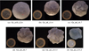 |
Fig. 2 3D printed grains with their corresponding technical name. |
Analog grain properties.
Grain radii.
3.2 Measurements
Laboratory measurements of complex transmission coefficients were performed in the anechoic chamber of the Centre Commun de Ressources en Micro-Ondes in Marseille to obtain the electromagnetic field scattered by the grains. These measurements were made with two antennas, with wavelengths ranging from 16.7 mm to 100 mm. Both antennas were used with the same state of polarization, both horizontally and then both vertically (copolarization). The emitter antenna was at a fixed position, while the receiving antenna moved and measured at different scattering angles, from θ = −130° to θ = 130°. This type of experimental setup in the forward-scattering zone was explained and illustrated in Fig. 2 in Tobon Valencia et al. (2022).
After measuring the transmission coefficients, calibrations were performed to obtain the scattered field. Then, the drift correction procedure (Eyraud et al. 2006; Bucci & Franceschetti 1987) was applied to finally derive the two copolarized Jones matrix elements, S1 and S2, and to translate them into the Mueller matrix elements of interest (based on Eqs. (7)–(12)).
The electromagnetic fields scattered by the grains were measured at different orientations to represent randomly oriented objects. Following the method described in Renard et al. (2021), the number of orientations was selected to guarantee convergence when the orientation-averaged Mueller matrix elements were computed. The number of orientations depends on the quantity of interest that is to be estimated and on the size dimension X of the grain. We needed between 20 ± 10 orientations for the smoothest grain (Gr_n10_r2.6) to 70 ± 10 orientations for Gr_n2_r13.2 to obtain an accuracy of 1% for the phase function. For DLP, we needed between 13 ± 10 to 44 ± 10 orientations to reach an accuracy of 1%. Thus, we used 72 orientations for Gr_n2_r13.3, Gr_n2_r13.2, and Gr_n4_r6.7 and 36 orientations for the remaining grains to compute all the orientation-averaged quantities.
3.3 Numerical simulation and cross-polarization terms
Simulations were made based on a FEM method with a dedicated code (Voznyuk et al. 2015), as explained in Tobon Valencia et al. (2022). A mesh conforming to the geometry was produced from the CAD file. A perfectly matching layer (PML) was added to the geometry in order to mimic an infinite computational domain. In the interest of correctly meshing the roughness, the object was discretized with a constant characteristic length regardless of the value of X, and this corresponded to λ/10 for the highest value of X. The width of the PML layer was λ/3, with a mesh resolution of about λ/10. The weak form of the Helmholtz equation was discretized into a set of edge elements. The total number of degrees of freedom of the linear system varied between 5.5 × 10⁵ (X = 1.24) and 7.7 × 10⁵ (X = 7.7). The sparse linear system was solved using a direct solver (Schenk & Gärtner 2011). The amount of memory used varied between 16 and 25 GB, and the resolution time was about 100 s using 52 cores and openMP. Our numerical computations were performed using the same geometric files of the 3D grains as were used for the 3D printing to simulate the co- and cross-polarized Jones matrix elements.
These FEM numerical simulations were used for three main purposes. First, to cross-validate the scattering properties of our grains. For this validation, the measured and simulated phase functions and DLP were compared (see Appendix A). Second, to verify the effect of including or excluding the cross-polarization terms in the scattering properties of interest (see Appendix B). Third, to analyze the behavior of the scattering properties in the angular ranges that cannot be reached via measurements.
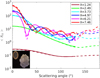 |
Fig. 3 Phase function of Gr_n2_r13.3 at different X values, measurements (solid lines), and simulations (dashed lines). |
4 Results and discussion
All our grains were measured and simulated with the necessary number of orientations to retrieve mean values of the Mueller matrix elements, as previously explained in Sect. 3.2. Five different scattering properties were analyzed for our grains and are presented in two different ways: first, the scattering properties of grains, and second, the scattering properties of grains weighted by size distribution.
4.1 Scattering properties of grains
The orientation-averaged scattering properties of our grains were studied at 6 different wavelengths: 100mm, 50mm, 33 mm, 25 mm, 20 mm, and 16.7 mm (out of a total of 16 wavelengths) and are expressed in terms of their corresponding size parameter, that is, between X = 1.07 to X = 7.73.
4.1.1 Phase function
Figure 3 presents the measured and simulated orientation-averaged phase functions for a single grain, that is, Gr_n2_r13.3, as an example at different wavelengths. The results for Gr_n2_r13.3 are shown here because it corresponds to the roughest of our grains. As all curves are calibrated, it is possible to vizualise the quantitative effects of the size dimension on the phase function. As expected, higher X values lead to higher forward-scattering values but smaller main-lobe widths. At low X values, a Rayleigh-like pattern arises, while at high X values, secondary lobes appear.
The measurements and simulations agree very well. To quantify these differences, we used the same comparison criterion as in Tobon Valencia et al. (2022) (a root mean square deviation normalized by the interquartile range, RMSDIQR). The values given by this comparison criterion can be found in Appendix A for each grain at different wavelengths.
The levels and curve shapes of the phase function at each wavelength are very similar for all the grains because the sizes between the grains do not change much (see the radius of the bounding sphere in Table 2 for each grain), as shown in Fig. 4, where the simulated phase function of all grains is superposed for the smaller wavelength λ = 16.7 mm. The grains were generated with the same initial sphere. The black curve in Fig. 4 represents the phase function of a sphere with the initial radius with which the grains were generated (r = 16.25 mm), showing that grains Gr_n10_r2.6 and Gr_n8_r3.4, that is, the smoothest grains, behave almost as perfect spheres. The main difference appears at high X because at high X, grains and their roughness are larger than the wavelength, meaning that the wave has a greater distance to travel inside the grain and therefore has more time to modify its waveform. Although there are differences, the curves behave in almost the same way in terms of levels and shapes regardless of the grain. This proves that the range of roughness that we used affects this scattering property only weakly.
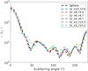 |
Fig. 4 Simulated phase functions for all grains at λ = 16.7mm corresponding to an average size parameter of Xmean = 6.94, and the simulated phase function of a sphere of r = 16.25 mm. |
4.1.2 Degree of linear polarization
Similarly, DLP measurements and simulations are consistent, as shown in fig. 5 for grain Gr_n2_r13.3, even though the differences between measurements and simulations are visually more important than for the phase function. This is further corroborated by the RMS DIQR values of DLP, which are higher than those of the phase function (see Appendix A). This can be explained by the phase function normalization factor 〈S11〉 whose discrepancy also increases with X.
For all grains, the DLP has the same Rayleigh behavior at the smallest X (brown line), while differences between grains DLP are more visible at the highest X values as oscillations appear. In Fig. 6, the simulated DLP at one of the highest X values is plotted for all the grains in order to show the influence of the irregular grain shape on the oscillations. For the smoothest grains (Gr_n10_r2.6 and Gr_n8_r3.4), the oscillations follow those of the sphere. Instead, for the two roughest and most anisotropic grain shapes (Gr_n2_r13.3 and Gr_n2_r13.2), the DLP starts to differ from that of a sphere. The roughest grains are the least spherical, while the smoothest grains are the most spherical (see Table 2). Thus, DLP seems to be a more appropriate parameter for distinguishing our grains according to their irregularity (convexity and/or shape anisotropy) when we compare their scattering properties.
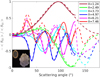 |
Fig. 5 DLP of Gr_n2_r13.3 at different X values, measurements (solid lines), and simulations (dashed lines). |
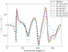 |
Fig. 6 Simulated DLP for all grains at λ = 20 mm, corresponding to an average size parameter of Xmean = 5.80, and the simulated DLP of a sphere of r = 16.25 mm. |
4.1.3 Other scattering properties
With the current observations made with telescopes, it is possible to obtain polarimetric images of protoplanetary and debris disks and retrieve the phase function and the DLP (see Van Holstein et al. (2020); Benisty et al. (2023), who retrieved 〈S12〉, and Tazaki & Dominik (2022) for DLP). Other scattering properties of protoplanetary disks are still not observable with current telescopes, however. Developments are ongoing at the Very Large Telescope (VLT) (Van Holstein et al. 2020) to derive, for example, the degree of circular polarization, with the issue that it is difficult to distinguish between the nonpolarized light from the star and the partially polarized light from dust. Assuming that only scattering mechanisms are involved and that randomly oriented particles are present, as in the present paper, we may be able to analyze other terms of the Mueller matrix. Thus, Appendix C presents the scattering properties 〈S22〉, 〈S34〉, and 〈S44〉. These properties will help us to understand and interpret the next generation of observations of the scattered-light images of protoplanetary disks.
4.2 Scattering properties of grains weighted by size distribution
As previously mentioned, the protoplanetary and debris dust sizes of interest to us are between 0.1µm to 10 µm. Grains with these dimensions will be efficient emitters in the optical and near-infrared (near-IR) range, but not in the millimeter range, as grains emit efficiently at wavelengths shorter than their physical size. Even so, there are observations of these disks which have millimeter emissions in Atacama Large Mil-limeter/submillimeter Array (ALMA) band 3, λ = 2.6 mm to 3.6 mm (see the example of the disk HL Tau observed in the ALMA Long Baseline Campaign, ALMA Partnership 2015), implying the presence of dust of about millimeter sizes. However, millimeter-sized dust is a poor emitter at near-IR and optical wavelengths when a power-law size distribution is considered. Therefore, this millimeter-sized dust can be neglected, and we considered a dust size range of 0.1 µm to 10 µm.
For micrometer-sized dust and optical wavelengths, the real dust size parameters would vary from Xmin = 0.90 to Xmax = 157. 08. Xmin is clearly very close to the mean minimum grain size parameter of Xinf = 1.16 (calculated with the mean radius of the bounding sphere of all grains at 18.45mm). Conversely, the mean maximum size parameter of our grains is Xsup = 6.94, which is not even in the orders of the real maximum dust size parameter. The probability of finding our maximum grain size parameter is still about 2% when we assume a power-law distribution in size. This means that grains with larger size parameters can be neglected because they are less likely to be present.
In the following, we weight all the scattering properties according to a power-law distribution in size in the following way:

The size parameter window was selected between Xinf = 1.16 and Xsup = 6.94. This power-law distribution can be applied because of our multiwavelength measurements and simulations. For each grain, we have access to 16 homothetic grain versions because we acquired the data at 16 different wavelengths, that is, at 16 different X values.
Additionally, for a complete analysis of how the index ns affects these scattering properties, two more power-law distributions with different indices were studied. Knowing that the supposed index is ns = 3.5, we decided to analyze the same scattering properties at a smaller and larger ns, thus, at X−2 and X−5. The reason was that a power law of ns = 3.5 is a supposition, not a certainty, and different authors therefore studied the scattering behavior at different indices, such as Zubko et al. (2015), who showed a stronger impact of the choice of index than the very particle morphology on these scattering properties.
4.2.1 Weighted phase function
A weighting according to the size distribution was applied to the different scattering properties of our grains, with varying ns values. The weighted phase functions of all six grains are shown in Fig. 7, where the measurements clearly match the simulations very well. The power-law distribution emphasizes the contribution of grains with low X values, that is, with a Rayleigh-like behavior. Therefore, the resulting phase functions do not present Mie-type oscillations, but a rather smooth profile.
At forward-scattering angles, the phase function curves are alike for a given ns, with smooth curves and similar half width at half maximum values (HWHM) regardless of the grain, as shown in Table 4. The radii of the bounding spheres of the grains are very close, and therefore, the sizes of their main scattering lobe are almost the same for a given ns. When ns increases, the HWHM becomes wider. This effect was expected because power-law distributions with larger coefficients give more weight to small X, hence to smaller grains, and consequently, to a larger angular aperture of the main scattering lobe. This behavior was also illustrated in Zubko et al. (2015), who performed the phase functions of irregularly shaped particles with a refractive index close to astronomical silicate (m = 1.6 + 0.0005i) with DDA simulations (with size parameters between X = 1–26) while changing the power-law index.
Instead, differences appear at backscattering angles. The levels reached at 180° are higher for the smoothest grains and decrease as the convexity and/or the shape anisotropy of the grains decreases, as shown in Fig. 8. To quantitatively appraise the variations in the backscattering levels, the gaps between the lowest point of each curve and the point at 180° are provided in Table 5 after the phase function was normalized at 0°. Two tendencies are visible: The backscattering level decreases either when ns increases or when the convexity and/or the shape anisotropy of the grain decreases. Hence, Gr_n10_r2.6, which is the smoothest and most convex grain, presents the highest phase function backscattering level when ns = 2. In sum, for a given ns, grains with different convexity and/or shape anisotropy can be differentiated by their backscattering levels. It is interesting to note here that the ordering in the backscattering zone of the normalized phase function is mainly correlated to the convexity of the grains, but not fully to their shape anisotropy.
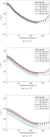 |
Fig. 7 Phase function weighted with a power-law distribution in size for different ns and different grains, measurements (solid lines), and numerical simulations (dashed lines). |
HWHM of the weighted phase function.
Backscattering levels of weighted phase functions.
4.2.2 Weighted degree of the linear polarization
The degree of linear polarization weighted with a power-law distribution in size is shown in Fig. 9 for different ns values and different grains. Two phenomena are identified depending on the power-law indices.
First, the maximum levels of DLP as well as their position change drastically with ns (see Table 6 for maximum DLP values for each grain). For ns = 2 ( ns = 3.5 and ns = 5), the maximum values are reached at scattering angles of 20° (85° and 98°). When ns increases, the maximum DLP value increases simultaneously, as does its position angle. ns controls the trade-off between the influence of small-size grains exhibiting Rayleigh-like behavior with a high DLP around 90°, on the one hand, and of large grains with a Mie-like behavior with strong DLP oscillations at lower scattering angles, on the other hand, as shown in Fig. 5. Low ns values favor low X values and therefore Rayleigh-like behavior, while large ns favors high X values and therefore Mie-like behavior.
Second, the negative polarization branch, around 150°–160°, weakens as the values of ns increase. The localization in the scattering angle of this negative polarization branch shifts slightly toward 160° when ns increases. This behavior was also illustrated in Zubko et al. (2015).
For each value of ns , two grain groups can be differentiated: on one hand, the most distorted grains (Gr_n2_r13.3 and Gr_n2_r13.2) with the smallest negative polarization branches and the highest maximum DLP levels; and on the other hand, the smoothest or most spherical grains (Gr_n10_r2.6, Gr_n8_r3.4, Gr_n6_r4.7, and Gr_n4_r6.7) with the largest negative polarization branches and the lowest maximum DLP levels. Hence, based on this scattering properties, the convexity and shape anisotropy of the grains is revealed with two elements: the levels of maximum DLP, and the characteristics of the negative polarization branch.
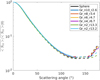 |
Fig. 8 Normalized phase function weighted with a power-law distribution in size with ns = 3.5 and for different grains, measurements (solid lines), and numerical simulations (dashed lines). |
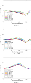 |
Fig. 9 DLP weighted with a power-law distribution in size for different ns and different grains, measurements (solid lines), and numerical simulations (dashed lines). |
4.2.3 Other weighted scattering properties
In Appendix D, the same power-law distribution in size is applied to the other scattering terms of the Mueller matrix, that is,  . The behaviors according to ns are similar to those observed for the weighted phase function. The observations also closely follow those in Appendix C.
4.2.4 Weighting on a larger size parameter window
So far, the chosen size distribution window was Xinf = 1.16 to Xsup = 6.94, which is a limited size distribution compared to reality. In protoplanetary disks, minimum size parameters can extend to Xinf = 0.1. Thus, for the purpose of understanding how a larger size parameter window may affect the weighted phase function and DLP, Appendix E covers a size parameter window from Xinf = 0.1 to Xsup = 6.94. This appendix proves that enlarging the size distribution window gives the same observed behaviors of the weighted phase function and the weighted DLP as described previously in Sects. 4.2.1 and 4.2.2.
5 Conclusions
The scattering behavior of six rough compact grains, ranging from X = 1 .07 to X = 7.73, were studied based on the scattering properties that we retrieved with our microwave-scattering measurements and FEM numerical simulations. These grains were designed and 3D printed as analogs of protoplanetary and debris dust grains. The morphological properties (shape anisotropy, convexity, etc.) of each grain were computed based on the CAD files that were shared between the 3D printer and the FEM mesh. The shape anistropy is directly related to grain sphericity, while convexity provides information about the grain smoothness.
Five elements of the Mueller matrix were analyzed for each grain: the phase function 〈S11〉 the degree of linear polarization −〈S12〉/〈S11〉, and 〈S22〉/〈S11〉, 〈S34〉/〈S11〉, and 〈S44〉/〈S11〉. The aim was to study how the grain morphology affected these scattering properties. All our measurements and simulations can be found in our database1.
Despite large size parameters X, which required much memory usage, we were able to simulate the scattering response of rough spheres with different levels of roughness, and this for reasonable calculation times because we used a numerical implementation of our FEM method on parallel architectures. The very good correspondence between the measured and simulated Mueller matrices demonstrated the accuracy of our measurement setup and the efficiency of our FEM simulations. The comparisons were based on calibrated results that showed that our calibration protocol is suitable.
Two types of studies were performed. First, we studied the scattering properties averaged over several orientations of grains at different wavelengths, corresponding to different size parameters. Among all the scattering properties, the DLP proved to be a good indicator of the grain morphology. With decreasing-convexity and/or shape anisotropy, the amplitude of the DLP oscillations increased. Moreover, 〈S22〉/〈S11〉 provided complementary information on the morphology of our grains, specifically, on their shape anisotropy, as 〈S22〉/〈S11〉 deviates farther away from 1 as their shape anisotropy decreases. This was previously observed in other studies of irregular particles (Li et al. 2004).
A second study was focused on using the same grain-scattering properties, but including a power-law distribution in size of the form  . Three power-law indices were used, ns = 2, 3.5, and 5. Three of all five scattering parameters presented characteristic behaviors related to roughness and sphericity, thus to the morphology of these grains, regardless of the ns value. First, the phase function presented ordered backscattering enhancements related to grain convexity, where the phase function of the smoothest (most convex) grain had the strongest enhancement and the roughest (less convex) grain had the lowest phase function. Second, the maximum DLP and negative polarization branches presented levels that were correlated to the grain shape anisotropy. Third,
  levels were also related to the shape anisotropy of our grains.
This first study of scattering properties of rough compact grains with controlled synthetic roughness is a first approach to understanding the light scattering of grains that was found in protoplanetary and debris disks. Nevertheless, the roughness of grains in nature is not synthetically controlled, as presented here. For this reason, future works will study the scattering properties of natural rough particles such as analogs of chondrules and calcium-aluminium-rich inclusions, which are elements of rocky meteorites or chondrites that participate in the planetary formation. The scattering properties of larger dust particles will also be investigated because they have gained significant attention in debris disks and in the Solar System (e.g., cometary dust or active asteroids).
Maximum level DLP.
Acknowledgements
This project was financially supported by CNRS, France, as part of its 80IPRIME cross-disciplinary programme. This work was also supported by the French National Research Agency in the framework of the Investissements d'Avenir program (ANR-15-IDEX-02), through the funding of the Cross-disciplinary Project "Origins of Life" of Univ. Grenoble-Alpes. It was also supported by the Programme National de Planetologie (PNP) of CNRS/INSU, France, also co-funded by Centre National d'Etudes Spatiales (CNES), France. Finally, this work is part of the Dust2Planets ERC-ADG-101053020 project. The authors would like to thank the Centre de Transferts de Technologie du Mans (CTTM) for the impression of the 3D grains. We would also like to thank “the Centre Commun de Ressources en Micro-Ondes” (CCRM) for providing the anechoic chamber and finally GDR Suie for the financial support.
Appendix A Comparison criteria for measurements and FEM simulations of the scattering properties
The comparison criterion used here was presented in Tobon Valencia et al. (2022). This criterion represents a quantitative estimation of the difference between our measurements and simulations. The comparison is based on a root mean square deviation (RMSD) calculus in which the simulation is taken as the reference. This criterion is normalized with the interquartile range (ƒßR) as follows: RMSDIQR = RMSD/(Q3 − Q1), Q3 being the 75th percentile and Q1 the 25th percentile.
The RMSDIQR is presented in Figures A.1–A.2 for the phase function and the DLP for all the grains. In gray, the same criterion compares an exact Mie calculus of a solid sphere with a radius of 16.25mm (initial radius of the sphere that was used to generate all grains) and a refractive index of 1.7 + i0.03, and the simulation of the same sphere with FEM. This gray line gives a reference of the minimum values that may be obtained with these FEM computations. Thus, when RMSDIQR values of the grains lie around this gray line, measurements and simulations agree well.
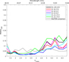 |
Fig. A.1 RMSDIQR of the phase function plotted for all the measured grains, taking their FEM simulation as reference. The gray line is a comparison of the Mie simulation vs. FEM computation with a sphere radius of 16.25 mm. |
For the phase function, the deviation is smaller than the gray line reference, up to Xmean = 4.25, showing a good agreement. Then, deviations increase for all grains up to RMSDIQR = 0.2. Two reasons can explain these deviations. First, increasing the grain size requires a finer mesh at smaller wavelengths. Second, for a larger grain size, the hypothesis of an incident plane wave illuminating the grain is less valid. The level of discrepancy between measurements and simulations is still fully satisfactory.
For the degree of linear polarization, the comparison criteria reach higher values than for the phase function. The acquisition of the DLP is thus more sensitive than the phase function. It is the ratio of two averaged Mueller matrix elements, which are both affected by measurements and simulations errors.
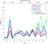 |
Fig. A.2 RMSDIQR of the DLP plotted for all the measured grains, taking their FEM simulation as reference. The gray line is a comparison of the Mie simulation vs. FEM computation with a sphere radius of 16.25 mm. |
Appendix B Influence of the co- and cross-polarized elements on the scattering properties
The FEM numerical simulations were used to verify the effect of including or excluding the cross-polarization terms in the scattering properties of interest. For this purpose, Figure B.1 presents the simulated scattering quantities with (dash-dotted lines) and without (dashed lines) cross-polarization, terms S3 and S4, for grain Gr_n2_r13.3.
The same comparison was made for the other grains, with similar conclusions. The influence of the cross-polarization increases as the size X of the scatterer increases. Nevertheless, these differences are negligible for all our grains, and our scattering quantities therefore only consider the copolarized elements S1 and S2, except for the simulated 〈S22〉, for which when the cross-polarized terms are excluded, 〈S22〉/〈S11〉 = 1.
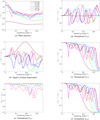 |
Fig. B.1 FEM numerical simulations of Gr_n2_r13.3, considering copolarized Jones matrix elements (dashed lines) and copolarized plus cross-polarized elements (thin solid lines) from X = 1.24 to X = 7.46. |
Appendix C Scattering properties 〈S22〉, 〈S34〉, and 〈S44〉
Three scattering properties different from the phase function and DLP were retrieved in order to validate (or observe other) scattering behaviors that were (or were not) seen by the phase function and DLP. These scattering properties are 〈S22〉, 〈S34〉, and 〈S44〉, which are described hereafter.
The simulated normalized parameter 〈S22〉/〈S11〉 is presented in Figure C.1 for grain Gr_n2_r13.3. This parameter is sensitive to shape anisotropy, as mentioned in Li et al. (2004), as 〈S22〉/〈S11〉 deviates from one when the shape anisotropy increases. In other words, a good indicator of asphericity is the degree to which the depolarization ratio  diverges from zero (Bottiger et al. 1980; Bohren & Huffman 1983). Figure C.1 shows that the deviation increases when X increases. The larger the particle, the more aspherical it is with respect to the wavelength.
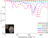 |
Fig. C.1 FEM simulated 〈S22〉/〈S11〉 for grain Gr_n2_r13.3 at different X values, including co- and cross-polarized Jones matrix elements. |
Figure C.2a presents 〈S22〉/〈S11〉 for all grains at λ = 100mm (Xmean = 1.16). For this low X value, grains behave like Rayleigh scatterers and all the curves tend to one, showing no difference at all. Conversely, when λ = 16.7 mm (Xmean = 6.94) (see Fig.C.2b), the grains become Mie-type scatterers. In this case, the curves deviate from one in an organized way from the two most spherical grains Gr_n10_r2.6 and Gr_n8_r3.4 to the two least spherical grains Gr_n2_r13.3 and Gr_n2_r13.2. This curves organization is in accordance with the sphericity indicator presented in Table 2. In this way, this scattering parameter adds scattering information compared to the phase function and DLP of our grains, providing information of the sphericity of grains.
Another parameter is 〈S44〉/〈S11〉, which is proportional to the degree of circular polarization (Bohren & Huffman 1983). This quantity is equal to 〈S33〉/〈S11〉, as shown in Fig. B.1, with and without cross-polarization. This equality highlights one of the Mie identities, 〈S33〉 = 〈S44〉, which is the case not only for spheres, but also for rough spheres, as reported in Li et al. (2004), and for radially homogeneous and inhomogeneous spheres, as noted in Dubovik et al. (2006). Our grains also exhibit this Mueller matrix identity. Figure C.3 presents 〈S44〉/〈S11〉 for grain Gr_n2_r13.3, where measurements and simulations behave similarly. At the smallest X (brown lines), 〈S44〉/〈S11〉 curves have soft falls, which is characteristic of Rayleigh scatterers, but for larger size parameters, the falls are composed of oscillations (Mie-like behaviors). This general behavior of soft falls for small X and oscillating falls for larger X is present for all grains and was already seen with DLP.
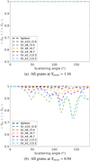 |
Fig. C.2 FEM simulated 〈S22〉/〈S11〉 for all grains including co- and cross-polarized Jones matrix elements at two different wavelengths (λ = 100mm and λ = 16.7mm). |
The normalized parameter 〈S34〉/〈S11〉 is illustrated in Figure C.3 for the roughest grain Gr_n2_r13.3. At the smallest X, the curve is almost constant, with values around zero for all the scattering angles. The same behavior is present for all the grains (Rayleigh behavior). For larger X, oscillations appear that reach up to ±0.7 for Gr_n2_r13.3. For other grains, the amplitude increases as the roughness decreases (Mie-like behavior) or the sphericity increases, reaching amplitudes of ±1 forGr_n10_r2.6. These two behaviors were already seen with DLP. This quantity therefore does not add any scattering information on our grains.
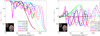 |
Fig. C.3 Normalized 〈S44〉/〈S11〉 and 〈S34〉/〈S11〉 for Gr_n2_r13.3 at different X values, measurements (solid lines), and numerical simulations (dashed lines). |
Appendix D Weighted scattering properties of 
The three other scattering properties weighted according to the size distribution are shown in the next figures, with varying ns values. The simulated scattering property  is presented in Figure D.1 for different ns values and different grains. As previously mentioned and shown in Appendix C, this quantity is related to the sphericity of the grains. The top-to-bottom organization of the curves, from more spherical to less spherical, can be directly correlated to their shape anisotropy ratio.
The scattering properties  are presented in Figure D.2 (Figure D.3) for different ns values and different grains. Changing ns mainly affects the behavior in the backscattering zone. For
  , the change in slope decay around 150° is more pronounced at low ns than at high ns values. For
  , the amplitude of the peak visible around 160° increases when ns decreases. Regardless of the grain type, the curves present the same characteristics. Consequently, these scattering properties do not provide any significant information for determining the level of convexity or shape anisotropy of our grains.
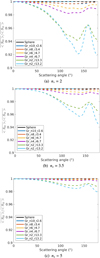 |
Fig. D.1
|

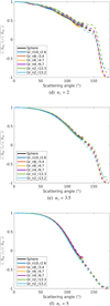 |
Fig. D.2
|

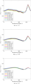 |
Fig. D.3
|

Appendix E Size distribution for smaller size parameters
In protoplanetary disks, the smallest size parameters can reach Xinf = 0.1. The scattering properties of X < 1 can easily be simulated by considering grains as spheres. This is possible because as the wavelengths increase, the details of roughness decrease, and so the whole grain can be considered as a sphere. In this section, we compute the two most important scattering properties, that is, the weighted phase function and the weighted DLP, while covering the size parameter window from Xinf = 0.1 to Xsup = 6.94 of the size distribution ns = 3.5. To do this, Mie simulations were performed from Xinf = 0.1 to X = 1.16 by taking the equivalent radius of each grain and simulating the scattering properties of their corresponding spheres. Then, from X = 1.16 to Xsup = 6.94, previous measurements and FEM simulations were taken. Finally, the phase function and DLP of ranges from Xinf = 0.1 to X = 1.16 and from X = 1.16 to Xsup = 6.94 were concatenated and a size distribution with an index ns = 3.5 was applied to obtain the weighted phase function and the weighted DLP on the entire size window range [0.1, 6.94](show in Figure E.1).
For the weighted phase functions, smooth profiles can be seen with wider HWHM values compared to weighted phase functions at ns = 3.5 in Figure 7. This effect was expected because a more realistic size distribution contributes more smaller grains, leading to a wider first lobe of the phase function. At backscattering angles, the same phenomena were observed with a smaller size window range. With decreasing backscatter-ing levels (gaps between the lowest point of each curve and the point at 180°), the grain convexity decreases as well.
For the weighted DLP, the maximum DLP levels have increased and the negative polarization branch levels have decreased compared to the weighted DLP with ns = 3.5 shown in Figure 9. This effect was once again expected because our the size distribution started at smaller size parameters, which gives more weight to a Rayleigh behavior. Although the size distribution window changed, however, the two least convex grains still have the highest maximum DLP levels and the smallest negative polarization branches. The same two grain groups can again be distinguished based on the maximum DLP and negative polarization branch levels, as mentioned in Section 4.2.2.
This appendix proved that even for a wider range of the size distribution, the weighted phase function and the weighted DLP still have the same observed behaviors as described in Section 4.2.1 and 4.2.2. The weighted phase function and weighted DLP we showed appear to be more similar in terms of values to those presented in Section 4.2.1 and 4.2.2 with a size distribution of index ns = 5. The reason for this is that applying a size distribution of ns = 5 with a size parameter window of Xinf = 1.16 to Xsup = 6.94 or that extending the size parameter window from Xinf = 0.1 to Xsup = 6.94 for a size distribution of ns = 3.5 has the same effect. They both provide the scattering information of small grains either by giving a larger weight to smaller grains or by extending the inferior window of the size distribution.
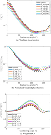 |
Fig. E.1 Weighted quantities with ns = 3.5 for a size window range [0.1, 6.94]. Mie simulations plus measurements are shown as solid lines, and Mie simulations plus FEM simulations are shown as dashed lines. |
References
- ALMA Partnership (Fomalont, E. B., et al.) 2015, ApJ, 808, L1 [Google Scholar]
- Angelidakis, V., Nadimi, S., & Utili, S. 2021, Comput. Phys. Commun., 265, 107983 [NASA ADS] [CrossRef] [Google Scholar]
- Bastien, P., & Menard, F. 1988, ApJ, 326, 334 [NASA ADS] [CrossRef] [Google Scholar]
- Bastien, P., & Menard, F. 1990, ApJ, 364, 232 [NASA ADS] [CrossRef] [Google Scholar]
- Benisty, M., Dominik, C., Follette, K., et al. 2023, in Protostars and Planets VII, eds. S. Inutsuka, Y. Aikawa, T. Muto, K. Tomida, & M. Tamura (San Francisco: Astronomical Society of the Pacific), ASP conf. Ser., 534, 605 [NASA ADS] [Google Scholar]
- Blum, J. 2018, Space Sci. Rev., 214, 52 [NASA ADS] [CrossRef] [Google Scholar]
- Bohren, C. F., & Huffman, D. R. 1983, Absorption and Scattering of Light by Small Particles (New York: John Wiley & Sons, Inc.), 544 [Google Scholar]
- Bottiger, J. R., Fry, E. S., & Thompson, R. C. 1980, in Light Scattering by Irregularly Shaped Particles, ed. D. W. Schuerman (New York: Plenum Pre, Springer), 283 [CrossRef] [Google Scholar]
- Bucci, O. M., & Franceschetti, G. 1987, IEEE Trans. Antennas Propag., 35, 1445 [CrossRef] [Google Scholar]
- Dohnanyi, J. S. 1969, J. Geophys. Res., 74, 2531 [Google Scholar]
- Draine, B. T. 2006, ApJ, 636, 1114 [Google Scholar]
- Draine, B. T., & Lee, H. M. 1984, ApJ, 285, 89 [NASA ADS] [CrossRef] [Google Scholar]
- Dubovik, O., Sinyuk, A., Lapyonok, T., et al. 2006, J. Geophys. Res. Atmos., 111, D11 [CrossRef] [Google Scholar]
- Escobar-Cerezo, J., Palmer, C., Muñoz, O., et al. 2017, ApJ, 838, 74 [NASA ADS] [CrossRef] [Google Scholar]
- Eyraud, C., Geffrin, J. M., Litman, A., Sabouroux, P., & Giovannini, H. 2006, Appl. Phys. Lett., 89, 244104 [NASA ADS] [CrossRef] [Google Scholar]
- Frattin, E., Muñoz, O., Moreno, F., et al. 2019, MNRAS, 484, 2198 [Google Scholar]
- Frattin, E., Martikainen, J., Mu, O., et al. 2022, MNRAS, 517, 5463 [NASA ADS] [CrossRef] [Google Scholar]
- Kahnert, M., Nousiainen, T., & Mauno, P. 2011, JQSRT, 112, 1815 [NASA ADS] [CrossRef] [Google Scholar]
- Kirchschlager, F., & Bertrang, G. H.-M. 2020, A&A, 638, A116 [NASA ADS] [CrossRef] [EDP Sciences] [Google Scholar]
- Li, C., Kattawar, G. W., & Yang, P. 2004, JQSRT, 89, 123 [NASA ADS] [CrossRef] [Google Scholar]
- Liu, C., Panetta, R. L., & Yang, P. 2014, Opt. Express, 22, 23620 [NASA ADS] [CrossRef] [Google Scholar]
- Liu, J., Yang, P., & Muinonen, K. 2015, JQSRT, 161, 136 [NASA ADS] [CrossRef] [Google Scholar]
- Mathis, J. S., Rumpl, W., & Nordsieck, K. 1977, ApJ, 217, 425 [NASA ADS] [CrossRef] [Google Scholar]
- Mishchenko, M. I. 2006, JQSRT, 101, 411 [NASA ADS] [CrossRef] [Google Scholar]
- Mishchenko, M. I., Hovenier, J. W., & Travis, L. D. 2000, Light Scattering by Nonspherical Particles (California: Academic Press), 690 [Google Scholar]
- Muinonen, K., Zubko, E., Tyynelä, J., Shkuratov, Y. G., & Videen, G. 2007, JQSRT, 106, 360 [NASA ADS] [CrossRef] [Google Scholar]
- Muinonen, K., Nousiainen, T., Lindqvist, H., Muñoz, O., & Videen, G. 2009, JQSRT, 110, 1628 [NASA ADS] [CrossRef] [Google Scholar]
- Mukai, S., Mukai, T., Giese, R. H., Weiss, K., & Zerull, R. H. 1982, Moon Planets, 26, 197 [NASA ADS] [CrossRef] [Google Scholar]
- Muñoz, O., Moreno, F., Vargas-Martín, F., et al. 2017, ApJ, 846, 85 [CrossRef] [Google Scholar]
- Muñoz, O., Moreno, F., Gómez-Martín, J. C., et al. 2020, ApJS, 247, 19 [CrossRef] [Google Scholar]
- Nousiainen, T., & Muinonen, K. 2007, JQSRT, 106, 389 [NASA ADS] [CrossRef] [Google Scholar]
- Pawellek, N., & Krivov, A. V. 2015, MNRAS, 454, 3207 [Google Scholar]
- Renard, J.-B., Hadamcik, E., Couté, B., Jeannot, M., & Levasseur-Regourd, A. C. 2014, JQSRT, 146, 424 [NASA ADS] [CrossRef] [Google Scholar]
- Renard, J.-B., Geffrin, J.-M., Tobon Valencia, V., et al. 2021, JQSRT, 272, 107718 [NASA ADS] [CrossRef] [Google Scholar]
- Schenk, O., & Gärtner, K. 2011, in Encyclopedia of Parallel Computing, ed. D. Padua (Boston, MA: Springer US), 1458 [Google Scholar]
- Sun, W., Nousiainen, T., Muinonen, K., et al. 2003, JQSRT, 79, 1083 [CrossRef] [Google Scholar]
- Tazaki, R., & Dominik, C. 2022, A&A, 663, A57 [NASA ADS] [CrossRef] [EDP Sciences] [Google Scholar]
- Testi, L., Birnstiel, T., Ricci, L., et al. 2014, in Protostars and Planets VI, eds. H. Beuther, R. S. Klessen, C. P. Dullemond, & T. Henning (Tuscon: University of Arizona Press), 339 [Google Scholar]
- Tobon Valencia, V., Geffrin, J.-M., Ménard, F., et al. 2022, A&A, 666, A68 [NASA ADS] [CrossRef] [EDP Sciences] [Google Scholar]
- Van Holstein, R. G., Girard, J. H., De Boer, J., et al. 2020, A&A, 633, A64 [NASA ADS] [CrossRef] [EDP Sciences] [Google Scholar]
- Voznyuk, I., Tortel, H., & Litman, A. 2015, IEEE Trans. Antennas Propag., 63, 2604 [CrossRef] [Google Scholar]
- Yada, T., Abe, M., Okada, T., et al. 2022, Nat. Astron., 6, 214 [NASA ADS] [CrossRef] [Google Scholar]
- Zerull, R. 1985, Int. Astron. Union Coll., 85, 197 [Google Scholar]
- Zhang, J., Bi, L., Liu, J., et al. 2016, JQSRT, 178, 325 [NASA ADS] [CrossRef] [Google Scholar]
- Zubko, E., Shkuratov, Y., & Videen, G. 2015, JQSRT, 150, 42 [NASA ADS] [CrossRef] [Google Scholar]
All Tables
All Figures
|
Fig. 1 Example of the virtual generation of our grains, where r is the initial radius of the sphere to mesh, rrough are the perturbed distances from the center of the sphere r to each triangle vertex, and Rmax is the radius of the bounding sphere, called maximum radius. |
| In the text | |
|
Fig. 2 3D printed grains with their corresponding technical name. |
| In the text | |
|
Fig. 3 Phase function of Gr_n2_r13.3 at different X values, measurements (solid lines), and simulations (dashed lines). |
| In the text | |
|
Fig. 4 Simulated phase functions for all grains at λ = 16.7mm corresponding to an average size parameter of Xmean = 6.94, and the simulated phase function of a sphere of r = 16.25 mm. |
| In the text | |
|
Fig. 5 DLP of Gr_n2_r13.3 at different X values, measurements (solid lines), and simulations (dashed lines). |
| In the text | |
|
Fig. 6 Simulated DLP for all grains at λ = 20 mm, corresponding to an average size parameter of Xmean = 5.80, and the simulated DLP of a sphere of r = 16.25 mm. |
| In the text | |
|
Fig. 7 Phase function weighted with a power-law distribution in size for different ns and different grains, measurements (solid lines), and numerical simulations (dashed lines). |
| In the text | |
|
Fig. 8 Normalized phase function weighted with a power-law distribution in size with ns = 3.5 and for different grains, measurements (solid lines), and numerical simulations (dashed lines). |
| In the text | |
|
Fig. 9 DLP weighted with a power-law distribution in size for different ns and different grains, measurements (solid lines), and numerical simulations (dashed lines). |
| In the text | |
|
Fig. A.1 RMSDIQR of the phase function plotted for all the measured grains, taking their FEM simulation as reference. The gray line is a comparison of the Mie simulation vs. FEM computation with a sphere radius of 16.25 mm. |
| In the text | |
|
Fig. A.2 RMSDIQR of the DLP plotted for all the measured grains, taking their FEM simulation as reference. The gray line is a comparison of the Mie simulation vs. FEM computation with a sphere radius of 16.25 mm. |
| In the text | |
|
Fig. B.1 FEM numerical simulations of Gr_n2_r13.3, considering copolarized Jones matrix elements (dashed lines) and copolarized plus cross-polarized elements (thin solid lines) from X = 1.24 to X = 7.46. |
| In the text | |
|
Fig. C.1 FEM simulated 〈S22〉/〈S11〉 for grain Gr_n2_r13.3 at different X values, including co- and cross-polarized Jones matrix elements. |
| In the text | |
|
Fig. C.2 FEM simulated 〈S22〉/〈S11〉 for all grains including co- and cross-polarized Jones matrix elements at two different wavelengths (λ = 100mm and λ = 16.7mm). |
| In the text | |
|
Fig. C.3 Normalized 〈S44〉/〈S11〉 and 〈S34〉/〈S11〉 for Gr_n2_r13.3 at different X values, measurements (solid lines), and numerical simulations (dashed lines). |
| In the text | |
|
Fig. D.1
|
| In the text | |
|
Fig. D.2
|
| In the text | |
|
Fig. D.3
|
| In the text | |
|
Fig. E.1 Weighted quantities with ns = 3.5 for a size window range [0.1, 6.94]. Mie simulations plus measurements are shown as solid lines, and Mie simulations plus FEM simulations are shown as dashed lines. |
| In the text | |
Current usage metrics show cumulative count of Article Views (full-text article views including HTML views, PDF and ePub downloads, according to the available data) and Abstracts Views on Vision4Press platform.
Data correspond to usage on the plateform after 2015. The current usage metrics is available 48-96 hours after online publication and is updated daily on week days.
Initial download of the metrics may take a while.