| Issue |
A&A
Volume 687, July 2024
|
|
|---|---|---|
| Article Number | A17 | |
| Number of page(s) | 10 | |
| Section | Astrophysical processes | |
| DOI | https://doi.org/10.1051/0004-6361/202449679 | |
| Published online | 24 June 2024 | |
The power of binary pulsars in testing Gauss-Bonnet gravity
1
Department of Theoretical Physics, Faculty of Physics, Sofia University, Sofia 1164, Bulgaria
e-mail: This email address is being protected from spambots. You need JavaScript enabled to view it.
; This email address is being protected from spambots. You need JavaScript enabled to view it.
2
Theoretical Astrophysics, Eberhard Karls University of Tübingen, Tübingen 72076, Germany
3
Institute of Mathematics and Informatics, Bulgarian Academy of Sciences, Acad. G. Bonchev St. 8, Sofia 1113, Bulgaria
4
INRNE – Bulgarian Academy of Sciences, 1784 Sofia, Bulgaria
Received:
20
February
2024
Accepted:
16
April
2024
Abstract
Context. Binary pulsars are a powerful tool for probing strong gravity that still outperform direct gravitational wave observations in a number of ways due to the remarkable accuracy of the pulsar timing. They can constrain the presence of additional charges of the orbiting neutron stars very precisely, leading to new channels of energy and angular momentum loss, such as scalar dipole radiation.
Aims. In the present paper, we explore in detail the possibility of constraining different classes of scalar-Gauss-Bonnet gravity with binary pulsars. Additionally, we updated the existing constraints related to the observed maximum mass of neutron stars.
Methods. Interestingly, depending on the equation of state, the resulting limits on the theory coupling parameters can outperform the constraints coming from binary merger observations by up to a factor of two, even for so-called Einstein-dilaton-Gauss-Bonnet gravity where neutron stars are often underestimated as relevant theory probes. As an additional merit, precise Bayesian methods are compared with approximate approaches, with the latter showing a very good performance despite their simplicity.
Key words: gravitation / gravitational waves / radiation mechanisms: general / stars: neutron / pulsars: general
© The Authors 2024
 Open Access article, published by EDP Sciences, under the terms of the Creative Commons Attribution License (https://creativecommons.org/licenses/by/4.0), which permits unrestricted use, distribution, and reproduction in any medium, provided the original work is properly cited.
This article is published in open access under the Subscribe to Open model. This email address is being protected from spambots. You need JavaScript enabled to view it. to support open access publication.
1. Introduction
Binary pulsars are among the first systems to allow the testing of general relativity (GR) in the strong field regime (Damour & Taylor 1991, 1992; Esposito-Farese 1996; Damour & Esposito-Farese 1996; Weisberg & Taylor 2005; Freire 2022). Different post-Keplerian parameters in the orbital motion of the neutron stars can be measured (Will 2014; Freire et al. 2001) and one of the most intriguing is related to the shrinking of the binary orbit due to gravitational wave emission. The observations fit very well the GR predictions and that is why modified theories of gravity possessing an additional channel of energy emission, attributed for example to the existence of a new fundamental field, are severely constrained (Kramer et al. 2021). A prominent example of a theory practically ruled out by the binary pulsar observations is the Damour-Esposito-Farese (DEF) model, which is a subclass of the massless scalar-tensor theories (STT) (Damour & Esposito-Farese 1992, 1993; Shao et al. 2017; Chiba 2022; Zhao et al. 2022)1. It outperforms by far the constraints based directly on the neutron star mass and radius observations (Tuna et al. 2022). In the DEF models, the additional channel of energy loss is controlled by the scalar charge (the coefficient in front of the leading order 1/r scalar field asymptotic at infinity), leading to scalar dipole radiation. Constraints on the DEF model were confirmed by a Bayesian analysis that employed a more sophisticated equation of state (EoS) and post-Keplerian parameters treatment (Anderson et al. 2019) as well as new pulsar timing models (Batrakov et al. 2024). Interestingly, a careful comparison in Anderson et al. (2019) reveals that the sophisticated Bayesian approach leads to very similar results to the simpler treatment employed in the past (Damour & Esposito-Farese 1996; Freire et al. 2012).
Another well-motivated class of extended STTs in which neutron star solutions were well studied is scalar-Gauss-Bonnet (sGB) gravity. Being more complicated than the DEF model due to the addition of a second-order (Gauss-Bonnet) curative invariant, it can be considered as an effective field theory that is motivated motivated by quantum gravity. It brings new interesting phenomenology such as the violation of the black hole no-scalar hair theorems (Mignemi & Stewart 1993; Kanti et al. 1996; Torii et al. 1997; Pani & Cardoso 2009). Two major classes of sGB theories became popular in the literature. The first one is the shift-symmetric theory with a linear coupling between the scalar field and the Gauss-Bonnet invariant for which black holes are always endowed with a scalar field. It can be considered as a leading order expansion of the so-called Einstein-dilaton-Gauss-Bonnet (EdGB) gravity in the case of a weak coupling (Mignemi & Stewart 1993; Kanti et al. 1996; Torii et al. 1997; Pani & Cardoso 2009). Neutron star solutions in these theories were constructed both in the static and rapidly rotating regimes (Pani et al. 2011; Kleihaus et al. 2014, 2016). Another interesting class of sGB theories admits so-called curvature-induced spontaneous scalarization (Doneva & Yazadjiev 2018a; Silva et al. 2018; Antoniou et al. 2018), analogous to neutron star spontaneous scalarization in the DEF model (Damour & Esposito-Farese 1992). Neutron stars in this case were obtained only in the static limit (Silva et al. 2018; Doneva & Yazadjiev 2018b; Xu et al. 2022).
Gravitational wave constraints on sGB gravity were addressed mainly in the context of black hole-black hole (Perkins et al. 2021; Wong et al. 2022; Wang et al. 2021; Tahura & Yagi 2018; Yamada et al. 2019) and black hole-neutron star (Lyu et al. 2022) merger events. Constraints of sGB gravity through binary pulsars are still scarcely studied, with the only exception being (Danchev et al. 2022), where the sGB gravity admitting spontaneous scalarization was adopted, and (Yagi et al. 2016), where a EdGB theory with a particular coupling function was considered. One of the reasons is that in shift-symmetric sGB gravity, neutron stars do not possess a scalar charge (Yagi et al. 2016); thus, the orbital decay will be the same as in GR. Moving from a linear scalar field coupling, like in the shift-symmetric case, to the exponential coupling in the EdGB gravity eventually leads to a scalar charge development (see Kleihaus et al. 2014, 2016) that alters the binary dynamics. Studying the induced constraints on EdGB gravity is one of the goals of the present paper.
Contrary to previous studies (Danchev et al. 2022), we do not perform a full Bayesian analysis, but instead a simpler and more tractable algorithm is developed for deriving constraints similar to the original studies in the DEF model (Damour & Esposito-Farese 1996; Freire et al. 2012). Estimating the power of this treatment is another goal.
A complementary approach for constraining the sGB gravity is through the existence of solutions. It is well known that neutron stars in sGB gravity possess a lower maximum mass compared to GR (for the same EoS) (Pani et al. 2011; Doneva & Yazadjiev 2018b). This allows us to set additional constraints on the parameters of the theory by taking into account the maximal observed neutron star mass up to now (Pani et al. 2011). We update previous results by considering the most recent neutron star observations with higher neutron star masses and compare them to the constraints coming from binary pulsars.
The paper is structured as follows: in Sect. 2 we shortly introduce the Gauss-Bonnet gravity. We continue in Sect. 3 with the description of the two methods that we adopted to constrain the theory. The results are presented in Sect. 4. The paper ends with a conclusion.
2. scalar-Gauss-Bonnet gravity
2.1. Basic equations
In the present paper, we study neutron stars in scalar-Gauss-Bonnet gravity. The general form of the action can be written as
![Mathematical equation: $$ \begin{aligned} S &= \frac{1}{16\pi }\int d^4x \sqrt{-g} \Big [R - 2\nabla _\mu \varphi \nabla ^\mu \varphi - V(\varphi ) + \lambda ^2 f(\varphi )\mathcal{R}^2_{\mathrm{GB}} \Big ] \nonumber \\&+ S_{\rm matter} (g_{\mu \nu },\chi ), \end{aligned} $$](/articles/aa/full_html/2024/07/aa49679-24/aa49679-24-eq1.gif) (1)
(1)
where R is the Ricci scalar and ∇μ is the covariant derivative with respect to the metric gμν. V(φ) is the scalar field potential and f(φ) controls the dimensionless part of the coupling between the scalar field, φ, and the Gauss-Bonnet invariant,  . Throughout this paper, we assume V(φ) = 0, while the particular choices of f(φ) are commented on in detail below. The Gauss-Bonnet coupling constant, λ, has a dimension of length. Smatter is the matter action.
The field equations derived from the action Eq. (1) are
 (2)
(2)
 (3)
(3)
where  is the matter energy momentum tensor. Γμν is defined by
 (4)
(4)
with
 (5)
(5)
The equation for hydrostatic equilibrium of the fluid can be derived from the Bianchi identity,
 (6)
(6)
In the present paper, we study static and spherically symmetric spacetime and a static and spherically symmetric scalar field and fluid configuration. For the spacetime metric, we adopt the standard ansatz:
 (7)
(7)
We set the matter source to be a perfect fluid with  , where ρ, p, and uμ are the energy density, pressure, and 4-velocity of the fluid, respectively. For the explicit form of the dimensionally reduced field equations and the equation for hydrostatic equilibrium, we refer the interested reader to Doneva & Yazadjiev (2018b).
To model a neutron star, an EoS should be specified. In the present paper, we use different realistic EoSs, represented through their piecewise polytropic approximation (Read et al. 2009). The specific EoSs we employ are commented on below.
The boundary conditions are the natural ones – regularity at the center of the star:
 (8)
(8)
and asymptotic flatness at spacial infinity:
 (9)
(9)
Typically in sGB gravity, the regularity at the stellar center fails to be fulfilled for large central energy densities. Therefore, the scalarized branches of solutions are terminated at a fixed maximum value of ρ. This is governed by the following regularity condition:
 (10)
(10)
where φ0, ρ0, p0, Λ2 are the coefficients in expansion at the stellar center,
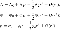 (11)
(11)
Equation (10) constitutes a fourth-order algebraic equation for Λ2 that depends on the central values of the pressure, p0, the energy density, ρ0, and the scalar field, φ0. In case no real roots for Λ2 exist, there are no regular neutron stars.
2.2. The coupling function
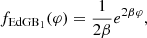
We are interested in two flavors of sGB theories. The first one is the EdGB gravity having  . More specifically, we focus on
 (12)
(12)
where β is a parameter. According to Eq. (3), φ = const is not a solution of the field equations in this case and compact objects are always endowed with a scalar field.
The particular normalization used in Eq. (12) is related to the fact that the leading order expansion with respect to φ is f(φ)∼φ. Thus, it is more straightforward to separate the contribution from the dimensional part of the coupling, λ, and the dimensionless parameter, β. Often in the literature, though, a slightly different normalization is considered; namely (Pani et al. 2011; Kleihaus et al. 2014, 2016),
 (13)
(13)
Clearly, this is a very slight modification of the coupling function that can be absorbed by rescaling the parameter λ in the following way:  . For practical reasons only, we also give some of the final theory constraints in terms of the coupling Eq. (13).
The second type of coupling function is associated with sGB theories admitting spontaneous scalarization that has  and
and  . The former condition secures that φ = const is a solution of the field equations. The latter offers a mechanism of destabilizing the GR-like compact object (for strong enough spacetime curvature) giving rise to a nontrivial scalar field configuration. The couplings we focus on are
 (14)
(14)
and
 (15)
(15)
Even though the two differ by just a minus sign, the solution properties are very distinct. While neutron stars can scalarize for both fSS1 and fSS2, static black holes can only develop a nontrivial scalar field for fSS2. The coefficients in the coupling function are adjusted in such a way that the leading order expansion is ±φ2.
3. Methodology
In the present paper, we combine the two most relevant methods of setting constraints on the sGB gravity through neutron star observations related to the maximum neutron star mass and the orbital decay of binary compact objects. Both constraints are related to pulsar timing observations because the most massive neutron star up to date is observed as a pulsar in a binary.
3.1. Constraints through maximum neutron star mass
The first approach is very straightforward and refers to the observation that the branches of solution (possessing nontrivial scalar fields) in sGB gravity typically have a smaller maximum mass compared to GR. The reason for this is twofold. First, the scalarized branches of solutions are terminated at some finite central energy density due to the violation of the regularity condition Eq. (10) that depends on the parameters (λ, β) (Pani et al. 2011). Thus, it can easily happen that the branch is terminated before the appearance of a turning point in the mass-central energy density dependence that can significantly lower the maximum allowed mass. Even if this does not happen for the chosen combination of (λ, β) and EoS, one should take into account the following. For a given central energy density, a GR neutron star typically has a larger mass than its scalarized counterpart. Thus, the maximum mass of the sGB neutron stars, for a given EoS, is smaller.
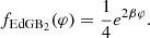
To help better understand this, in Fig. 1 we present a mass of radius relation for the two types of couplings discussed above. The top panel depicts sGB gravity with spontaneous scalarization (coupling function fSS1 Eq. (14)), and the bottom panel the EdGB theory (coupling function fEdGB1 Eq. (12)). The parameters were chosen to better visualize the different types of branches – the ones terminated at relatively small maximum mass and the “longer” ones that are reaching a turning point but that still have a maximum mass below GR. As one can notice in the case of spontaneous scalarization (top panel), there is a bifurcation point below which no scalarized solutions exist and the only stable solution is the GR one. For a given EoS, this bifurcation point depends only on the Gauss-Bonnet coupling constant, λ, and not on β. In the case of EdGB gravity (bottom panel), no bifurcation point is present and GR is not a solution of the field equations.
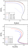 |
Fig. 1. Mass of radius relation for sequences of neutron stars with the MPA1 EoS in sGB gravity. The theory parameters were chosen to demonstrate the different types of branch behavior and their influence on the maximum mass. Top: Gauss-Bonnet gravity with scalarization (coupling function fSS1). Bottom: EdGB gravity (coupling function fEdGB1). |
To constrain sGB theory, one should simply require that a neutron star solution with the observed maximum mass is allowed for a given set of theory parameters. Of course, the results will be also EOS-dependent. This approach has already been employed in Pani et al. (2011) where constraints on a combination of λ and β were derived. However, newer observations supply us with an updated larger maximal neutron star mass that will eventually set tighter constraints on the theory. In addition, the scalar field coupling functions (f(φ)) that we consider are more general compared to Pani et al. (2011).
3.2. Constraints through orbital decay of binaries
The second, more sophisticated method of probing sGB gravity is based on the observed orbital decay of the binary pulsars. In sGB gravity the shrinking of the orbit will be sped up by the emission of scalar dipole radiation, in case of a nonzero scalar field charge. This will manifest itself as an excess in the orbital decay compared to GR. The excess can be measured through pulsar timing observation and up to now it has been consistent with zero within the observational accuracy (Wex & Kramer 2020); thus, no deviation from GR can be confirmed2.
As we noted, scalar dipole radiation is emitted only for a neutron star with a nonzero scalar charge, defined as the coefficient in front of the leading order, 1/r, asymptotic at infinity. For a faster-decaying scalar field (e.g., 1/r2 or an exponential decrease observed, for example, for a massive scalar field), the scalar charge is zero despite the presence of a strong scalar field in the vicinity of the compact object. Thus, observations of the orbital decay eventually set constraints not directly on the presence of a scalar field, but rather on the value of the neutron star scalar charge. In sGB gravity, the presence or absence of a nonzero scalar charge is controlled by the particular choices of f(φ) and V(φ).
Contrary to gravitational radiation in GR, which is quadrupolar tensorial radiation, in sGB there is additional scalar radiation that has monopol, dipolar, and quadrupolar components. Typically for a binary pulsar in sGB gravity, the dipolar one dominates, followed by the quadrupolar one. In our studies, we take into account only the former one, which is a good first approximation. The change in the orbital period of the binary system, Pb, associated with the scalar dipolar radiation has the form (Damour & Esposito-Farese 1992, 1996)
 (16)
(16)
where Dp is the dilaton charge of the primary pulsar, Dc is the dilaton charge of the companion (typically either a neutron star (NS) or a white dwarf (WD)), mp and mc are the masses of the pulsar and its companion, and e is the eccentricity of the binary orbit. From the above expression, it is clear that for the dipolar emission to be strong not only the scalar charge has to be large but also the ratios Dp/mp and Dc/mc have to be significantly different (e.g., an equal mass binary neutron star system will still have zero scalar dipole radiation). In the present paper, we focus predominantly on cases in which only the primary pulsar has scalar hair, while the companion is a non-scalarized white dwarf that has negligible Dc. Such systems give for the moment the strongest constraints on sGB gravity (Danchev et al. 2022).
When interpreting observations, one should proceed in the following way. First, all kinematic effects (the relative acceleration between the binary and the Solar System barycenter along the line of sight, the Shkolovskii effect, the mass loss of the system, the tidal effects, and the possible variation in the gravitational constant on a cosmological timescale) should be subtracted from the observed total orbital decay rate (Ṗb) (Damour & Taylor 1991). This would give us the intrinsic orbital decay,  , which is the total orbital energy lost due to gravitational radiation (denoted by
  with a dominant quadrupolar contribution) and potentially scalar radiation (mainly the scalar dipolar one,
  ). When the gravitational contribution is subtracted from the intrinsic orbital decay, the result is the so-called “excess” orbital decay,
  :
:
 (17)
(17)
Thus, measuring  will give us an upper limit on the scalar dipolar radiation and eventually constrain the scalar charges through Eq. (16).
The ultimate approach one can follow is to perform a Bayesian analysis, taking into account all of the observational uncertainties in the observed quantities such as  , the pulsar mass, etc. (Danchev et al. 2022) (or even to perform a more sophisticated data analysis Batrakov et al. 2024). Since simpler classical methods (Damour & Esposito-Farese 1996; Freire et al. 2012) have shown a comparably good performance to the Bayesian analysis for the DEF model (Anderson et al. 2019), we were motivated to develop a procedure similar to Damour & Esposito-Farese (1996) but adjusted for sGB gravity. Namely, for each EoS we built a two-parametric family of solutions in a (λ, β) plane, having a constant mass equal to the mass of the observed pulsar. Practically speaking, for each combination of λ and β we searched for a central energy density, ρc, that produces a neutron star model with the desired mass. For each neutron star model in this two-parametric family of solutions, one can compute the dipole radiation through Eq. (16) and compare it with the orbital decay excess,
  , for the given binary. Clearly, there exists a line that separates regions where
  and vice versa. Practically speaking, this line gives us a β dependent constraint on the parameter λ (or vice versa). This procedure is much more straightforward and requires much less computational effort than a Bayesian analysis.
4. Results
Before commencing the presentation of our results, we shall summarize the data for the binary systems we are going to study. In Table 1 we list the main parameters of the binary pulsar systems that we adopt in the orbital decay study. Those are the three systems studied in Danchev et al. (2022), with one additional system that was found to also provide good constraints of EdGB gravity (Yagi et al. 2016). We strive for consistency with Danchev et al. (2022) because we used their statistical results as a reference for testing our methodology.
Parameters of the NS–WD pairs that were used to constrain the theory using the Ṗb method.
The heaviest-known neutron star up to now is the pulsar in the binary system J0952−0607, discovered in 2016 (Bassa et al. 2017). It is a “black widow” pulsar, the mass of which is estimated to be MNS = 2.35 M⊙ (Romani et al. 2022). Of course, there are uncertainties associated with this measurement and the data analysis shows that the pulsar mass should be > 2.09 M⊙ at a 3σ confidence level. This is the value that we adopt in the derivation of the maximum mass constraints on the theory. J0952−0607 is a relatively recently discovered pulsar, though, and to our knowledge there is no available data for the orbital decay rate of the system in the literature. We should note that the lower limit of 2.09 M⊙ that we employ is almost identical to the median mass of 2.08 M⊙ of J0740+6620, the second-most-massive known pulsar system (Fonseca et al. 2021).
For consistency with previous studies, the results in the rest of this section are presented in dimensionless units. The dimensionless Gauss-Bonnet coupling constant is defined as
 (18)
(18)
where  km is one half of the gravitational radius of one solar mass object. The constant, β, in the coupling functions is dimensionless by definition.
4.1. Constraints on sGB gravity admitting scalarization
We start our study with the case of sGB gravity admitting spontaneous scalarization. This case has already been extensively studied in Danchev et al. (2022), where Bayesian analysis was applied and the results for three binary pulsars and multiple EoSs are presented. In this section, we aim to demonstrate that the simpler methodology described above, and borrowed from the DEF model, is applicable to sGB gravity as well and there is a good agreement with the results from the statistical analysis. For comparative reasons, we focus on the two coupling functions, Eqs. (14) and (15), which were also employed in Danchev et al. (2022). The scalar field radial profile is very different in both cases (Doneva & Yazadjiev 2018b; Kuan et al. 2021) and consequently the binary pulsar constraints differ as well (Danchev et al. 2022). That is why it is important to consider both. Since we aim in this section to prove that the method can be applied and has a similar accuracy to the statistical one, only one pulsar (J0348+0432 from Table 1, which provides the most stringent constraints) and two EoSs are presented; namely, MPA1 (Müther et al. 1987) and WFF1 (Wiringa et al. 1988), which are representative examples allowing a maximal mass in GR above 2.09 M⊙ The two EoSs were chosen so that we could compare with (Danchev et al. 2022) and, on the other hand, of the set of EoSs used in the following section, they give the most relaxed and the most stringent constraints, respectively; hence, they are good representatives.
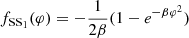
The results for the binary pulsar constraints on the parameters (λ, β) are given in Fig. 2. In both panels, the dashed line marks the critical value of λ at which the bifurcation point of the scalarized branch from the GR one is exactly at a mass equal to the mass of the pulsar. This line is independent of β. For λ below this line, no scalarized solutions with the desired mass exist, and therefore this region is not constrained from observations. The continuous line is the critical curve at which the scalar dipole radiation is equal to the excess in the orbital decay. Strictly speaking, the measured excess agrees with zero for all pulsars. What we have taken as an excess, though, is the maximum deviation from zero corresponding to the 1σ confidence level of each measurement. The area between the dashed and continuous lines is that part of the parameter space for which scalar dipole radiation is present, but it is lower than the excess. Summing up, the values of parameters situated below the solid line are allowed from observations. Moreover, we have explicitly checked that for all considered values of λ and β the constraints coming from the maximum observed neutron star mass are weaker than the one in Fig. 2.
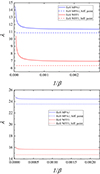 |
Fig. 2. Constraints on sGB gravity admitting scalarization, obtained from the orbital decay rate of J0348+0432 for two EoSs (depicted with solid lines). The dashed line denotes the threshold value of λ below which scalarized solutions exist only for neutron star masses above the pulsar one, and thus no constraints can be imposed. This limit is related to the bifurcation points in the top panel of Fig. 1 and is independent of β. Top: coupling function Eq. (14). Bottom: coupling function Eq. (15). |
We shall describe in more detail how the binary data was used and how we got those curves. For the bifurcation line, we used the median mass of the pulsar. This line was not used to set an actual constraint on the theory (at least for the coupling functions considered in the present subsection) but instead just indicates where scalar dipole radiation exists at all. For the continuous line, the procedure is the following. The scalar dipole radiation given by Eq. (16) depends on the scalar charge as well as the parameters of the system – the orbital period, the eccentricity, and the masses of the pulsar and its companion. All of the parameters of the system, though, are known with some uncertainty (Table 1). The uncertainty of the orbital period is negligible and can be ignored. The eccentricity is very small by itself and gives little contribution to Eq. (16). Therefore, using the median value from Table 1 and ignoring its uncertainty will leave our results practically unchanged. The mass of the pulsar, though, has a major impact on the dipole radiation, and varying it within the uncertainty interval leaves a clear effect on the theory constraints. Since a larger mass would typically give stronger constraints (while keeping the rest of the parameters fixed), the most orthodox approach is to employ in our studies the lower limit for the pulsar mass, that is mp = 1.9495 M⊙3. As far as the mass of the companion is concerned, what is important is to keep the mass ratio fixed because this is the parameter that is observed with a very high accuracy. Thus, we worked with mc = 0.1668 M⊙. The orbital decay excess was calculated as the intrinsic orbital decay from Table 1 minus the orbital decay predicted by GR from Antoniadis et al. (2013); that is,  at 1σ confidence, from which we took the lower bound. Through that procedure, one obtains a maximal possible excess of
  .
.
When compared with the results from the Bayesian analysis in Danchev et al. (2022), it is clear that the constraints derived by the two methods are almost identical, although, the statistical method provides more thorough information and probability for the parameters. This shows that the methodology developed for the DEF model is applicable to sGB gravity as well; at the same time, it is significantly less demanding from a computational point of view.
4.2. Constraints on Einstein-dilaton-Gauss-Bonnet gravity
The second class of sGB gravity that we consider is the so-called EdGB theory with an exponential coupling function given by Eq. (12). Often in the literature only the leading order expansion with respect to φ is considered, making f(φ) a linear function of φ. This corresponds to the shift-symmetric Gauss-Bonnet theory. It was proven, though, that in this case the scalar charge of neutron stars is identically zero. Hence, no constraints from binary pulsars can be imposed (Yagi et al. 2016). This observation is not true in the general case of an exponential coupling function such as Eq. (12). Indeed, in this case, the scalar charge will still be relatively small but the accuracy of the pulsar timing observations is constantly improving and it is thus interesting to check whether constraints based on the binary orbital decay are already comparable to the most up-to-date limits coming from binary merger observations (Yang et al. 2023). In addition, the constraints coming from the updated maximum neutron star mass observations (Romani et al. 2022) are independent of the scalar charge, and thus they apply to the shift-symmetric flavor of the theory as well.
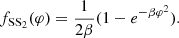
To calculate the constraints related to the orbital decay, we adopted the binaries presented in Table 1. We used the piecewise polytropic approximation (Read et al. 2009) of four different EoSs that allow for maximal masses larger than 2.09 M⊙ in GR (the lower 3σ confidence limit of the mass of J0952−0607); namely, MPA1 (Müther et al. 1987), APR3 (Akmal et al. 1998), APR4 (Akmal et al. 1998), and WFF1 (Wiringa et al. 1988). Constraints on the parameters (λ, β), using the coupling function Eq. (12), for all three pulsars, and fixed EoSs, are presented in Fig. 3. As was expected, as β → 0 the constraints get weaker because we get closer to the shift-symmetric theory with f(φ)∼φ, where the scalar charge is always zero for neutron stars. The pulsar J1012+5307 gives the least stringent constraints on the (λ, β) space, while the rest of the systems (J0348+0432, J2222−0137, and J1738+0333) lead to similar results. This is different from the couplings Eqs. (14) and (15), where the heaviest pulsar gives the most stringent constraints (Danchev et al. 2022). Instead, in EdGB gravity what plays a role is a combination of the pulsar mass and the accuracy of the  measurement.
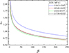 |
Fig. 3. Constraints on the parameters λ and β for four NS–WD pairs, based solely on dipole radiation due to the scalar field. The EdGB theory with coupling Eq. (12) is considered. |
In what follows, we predominantly focus on J0348+0432 and J2222−0137 as representative examples. We point out that for the latter system the white dwarf has a significantly higher mass compared to the rest. It is worth remembering that in this flavor of sGB gravity, any compact object will be endowed with a scalar field. As the compactness decreases, though, the source term for the scalar field – that is, the Gauss-Bonnet invariant – decreases very rapidly. Thus, the scalar charge even for such a high-mass white dwarf (which has a typical radius more than two orders of magnitude larger than a neutron star) can be safely neglected in comparison to the pulsar.
In Fig. 4 we proceed by comparing the constraints on the (λ, β) parameter space obtained by the orbital decay and maximal mass methods for two representative EoSs; namely, MPA1 and WFF1, and the binary J0348+0432. The dashed line corresponds to combinations of (λ, β) for which the maximal mass of the resulting sequence of beyond-GR neutron stars is exactly 2.09 M⊙. The solid line corresponds to the parameters for which the scalar dipole radiation of a J0348+0432-like system has some set numerical accuracy, equal to that given earlier in this section for  for this binary. The shaded blue area (the region above the dashed line) indicates the set of parameters for which the maximal mass M = 2.09 M⊙ cannot be reached, while the shaded gray area (the region above the solid line) indicates the part of the parameter space in which the scalar dipole radiation of the system is larger than the
  for the binary. In the white area are the parameters allowed by both methods. From the figures, it is clear that for small and high values of β the requirement for maximal neutron mass above 2.09 M⊙ dominates, which is natural since for β → 0 the scalar charge of the neutron stars is vanishingly small. For intermediate values of β, on the other hand, the
  measurement provides more relevant constraints.
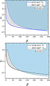 |
Fig. 4. Constraints on the λ − β parameter space based on maximal mass and orbital decay due to the emission of gravitational radiation for two EoSs. The EdGB theory with coupling Eq. (12) is considered. |
In Fig. 5 we study and compare the constraints on the parameters space for the four EoSs, MPA1, APR3, APR4, and WFF1. Results from the orbital decay for both J0348+0432 and J2222−0137 are presented for all four EoSs. The curves that separate the allowed part of the parameter space from the forbidden part were obtained by combining the two methods; the part of the curve related to the orbital decay is marked with a continuous line and the contribution from the maximal mass method is marked with a dashed line. The allowed parameters for a given EoS and binary are below the given curve. For more or less all values of β, the uncertainty in the EoS leads to the fact that the maximal allowed values for λ double from the EoS with the lowest lambda to the one with the highest.
 |
Fig. 5. Constraints on the parameters λ and β, based on two constraining methods, using different types of observational data and for four different EoSs. Results from the orbital decay for both J0348+0432 and J2222−0137 are presented for all four EoSs. The EdGB theory with coupling Eq. (12) is considered. In addition, the orange line marks the constraints coming from the existence of minimum mass black hole. Top: wide β range plot. Bottom: zoom-in of the constraints for small values of β. |
An interesting fact is that in EdGB gravity there is a minimal mass allowed for the black holes, which depends on the parameters of the theory. This happens due to a violation of the regularity conditions at the black hole horizon that is a relation similar to Eq. (10) for neutron stars. This by itself provides additional constraints on the parameter space, since the theory parameters should be such as to allow the existence of the minimum observed black hole mass. Currently, the gravitational wave observations show that the minimum black hole mass should be at least roughly Mbh = 5 M⊙ measured for the event GW190924_021846 (Abbott et al. 2021). This constraint is plotted as an orange line in the figure, marking the combinations of (λ, β) for which the minimal allowed mass for the sequence is exactly 5 M⊙. The allowed parameters are below this curve. It is clear that such a constraint strongly restricts the parameter space only for large values for β, while for small β the neutron star constraints prevail.
We now consider the coupling function Eq. (13). As we mentioned, it is equivalent to the coupling Eq. (12) through a redefinition of the parameter λ. Since it is widely used in the literature, though, it is useful to show a plot with the corresponding constraints. In Fig. 6 we present the combined constraints from the orbital decay and maximal mass methods for J0348+0432 and EoS WFF1 as well as the black hole constraint for the coupling Eq. (13). As could be expected, the values for λ are just rescaled with respect to the previous figures. It is interesting to point out that due to the nonlinear connection between the coupling constants, for small β the maximal allowed λ increases with the decrease in β, contrary to the coupling Eq. (12).
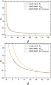 |
Fig. 6. Constraints on the parameter space λ – β, similar to Fig. 5, but for the EdGB theory with coupling Eq. (13). Top: wide β range plot. Bottom: zoom-in of the constraints for small values of β. |
In the end, we should see how our results compare with other available constraints in the literature. In Pani et al. (2011) the authors derive constraints on the parameters of EdGB gravity with exponential coupling by using the maximal mass of neutron stars. At that time M ≥ 1.93 M⊙, so clearly our constraints are stronger. In addition, we used the full form of the exponential coupling function, while in Pani et al. (2011) only the limit of small scalar fields, and thus weak coupling was considered. Recently, the maximal mass constraints on the sGB gravity were updated in the case of shift-symmetric Gauss-Bonnet gravity (Saffer & Yagi 2021) with a newer value for the maximal mass M = 2.01 M⊙. The most stringent constraint that the authors report in that paper is for EoS MPA1, which we use as well in the present work. They find (translated into our notations and dimensionless units) λ < 2.53, which is similar to our results in the β → 0 limit. This minor inconsistency can easily be explained by the fact that in Saffer & Yagi (2021) the authors used perturbative methods to solve the field equations, while we solved the field equations numerically with no simplifications. We should also note that for the selected set of EoSs, the constraints from the EoS MPA1 are the least stringent.
In Yagi et al. (2016) the authors derived constraints on EdGB gravity with exponential coupling from scalar dipole radiation from neutron star-white dwarf binaries. They employed Tolman VII and polytropic n = 0 models. In addition, the parameter in the coupling function exponent, denoted by γ in their notations, was set to 1. When translated into our notations and dimensionless units, γ = 1 corresponds to our β ∼ 0.14, and their final theory constraints for λ are between ∼2.5 and ∼5.1. Those constraints are weaker than our results and the reason is that for such small values of β the dominating constraints come from the maximal masses rather than scalar dipole radiation.
Similar constraints come from a recent work (Lyu et al. 2022) in which the authors study the constraints on EdGB gravity by analyzing the gravitational wave signal from black hole – neutron star binaries. They work in the small coupling approximation, which results in shift-symmetric Gauss-Bonnet gravity (f(φ) = φ). It is important to mention that constraints coming from the orbital decay are not possible in that case due to a zero scalar charge, and therefore zero scalar dipole radiation. The maximum neutron star mass constraints are valid, though, in this limit. In order to compare the results, we need to rewrite our action in the form that they use or vice versa. This requires a redefinition of the scalar field and a redefinition of the constants. Their combined bound  km translates into λ ≲ 4.44 km in our notation or λ ≲ 3.01 in the dimensionless units presented in the figures. It is clear that, depending on the EoS, the maximal values for the coupling constant that we get from the maximal mass constraint range from less than half of what they get up to values very similar to theirs. As for the constraints that we get from the minimal black hole mass, the maximal values for the coupling constant are in correlation with their results.
5. Conclusion
In the present paper, we aim to explore methods of constraining sGB gravity through observational data from binary pulsar systems. As a first step, we adjusted a simplified nonstatistical method of imposing constraints via observations of the orbital shrinking of binary pulsars. It is based on the idea of calculating the theoretical prediction of scalar dipole radiation for a given beyond-GR neutron star model and comparing it to the excess in the orbital decay. It was carefully demonstrated that it gives comparably good results to the previous, more sophisticated Bayesian analysis in sGB gravity admitting spontaneous scalarization. The second major constraint related to binary neutron stars is the observed maximal neutron star mass. Namely, the theory parameters should be adjusted in such a way that such a high-mass neutron star exists in our theory. Additionally, we included the constraints from the lowest observed black hole mass.
Focusing on EdGB theory, we should point out that, contrary to the known results in the literature, we did not explicitly impose from the beginning small field or small coupling approximations but instead employed the full exponential form of the coupling. This allowed us to properly study the two-dimensional parameter space made of the dimensional Gauss-Bonnet coupling constant, λ, and the parameter, β, in the coupling function exponent. On the other hand, this meant that no single value constraint on λ could be set and that, instead, it is dependent on β. In addition, the EoS plays a major role and the resulting constraints strongly depend on it. Limiting ourselves to some of the modern, widely accepted EOSs, though, we show that the end results vary by less than a factor of two.
A general observation is that EdGB gravity is best constrained by the maximum mass method for very large and very small values of the parameter β, while binary pulsar orbital decay provides the best limits for intermediate β. We should point out that, for the considered coupling, β → 0 tends to the shift-symmetric sGB theory with a linear coupling with respect to the scalar field. In that case, the scalar charge, and thus the scalar dipole radiation, are identically zero. Hence, the orbital decay approach cannot constrain the theory and it is natural that the maximum mass observations give the strongest limits there.
Very importantly, the derived constraints are either comparable or better than the ones coming from binary mergers (Lyu et al. 2022), with an improvement of up to a factor of two depending on the EoS. This is a very intriguing result because neutron stars are often overlooked as a probe of EdGB gravity.
Future observations will improve the precision of the parameters employed in the paper. Potentially, a higher maximum mass neutron star might be observed or the accuracy of the mass determination of what is currently the most massive pulsar can be improved. As far as the orbital decay is concerned, continuous observations of already known pulsars improve more and more the current bounds on the orbital decay excess. Therefore, we can expect that in the next decade the bounds derived in the present paper can be significantly improved. On the other hand, the binary merger observations are improving as well, and detecting a longer inspiral phase preceding the binary merger, due to increased sensitivity or a favorable high signal-to-noise ratio event, will improve the theory constraints derived in Lyu et al. (2022).
Note that a nonzero scalar field mass can evade the binary pulsar constraints (Ramazanoğlu & Pretorius 2016; Yazadjiev et al. 2016; Rosca-Mead et al. 2020), rapid rotation can magnify the deviations from GR considerably (Doneva et al. 2013), and other sectors of STTs are only weakly constrained by binary pulsars (Mendes & Ortiz 2016; Mendes & Ottoni 2019).
Note that in a recent paper (Wolf & Lagos 2020) the authors argue that the current constraints on the variation of the gravitational coupling and its effect on the binary pulsar period might not be accurate for some modified theories of gravity.
This value corresponds to the 1σ errors that is used to be consistent with previous studies of binary pulsar constraints in modified gravity (Shao et al. 2017; Danchev et al. 2022).
Acknowledgments
We would like to thank Kent Yagi, Norbert Wex, and Paulo Freire for reading the manuscript and useful suggestions. This study is in part financed by the European Union-NextGenerationEU, through the National Recovery and Resilience Plan of the Republic of Bulgaria, project No. BG-RRP-2.004-0008-C01. D.D. acknowledges financial support via an Emmy Noether Research Group funded by the German Research Foundation (DFG) under grant no. DO 1771/1-1.
References
- Abbott, R., (LIGO Scientific Collaboration & Virgo Collaboration) et al. 2021, Phys. Rev. X, 11, 021053 [Google Scholar]
- Akmal, A., Pandharipande, V. R., & Ravenhall, D. G. 1998, Phys. Rev. C, 58, 1804 [Google Scholar]
- Anderson, D., Freire, P., & Yunes, N. 2019, Class. Quant. Grav., 36, 225009 [NASA ADS] [CrossRef] [Google Scholar]
- Antoniadis, J., Freire, P. C. C., Wex, N., et al. 2013, Science, 340, 448 [Google Scholar]
- Antoniou, G., Bakopoulos, A., & Kanti, P. 2018, Phys. Rev. Lett., 120, 131102 [NASA ADS] [CrossRef] [Google Scholar]
- Bassa, C. G., Pleunis, Z., Hessels, J. W. T., et al. 2017, ApJ, 846, L20 [NASA ADS] [CrossRef] [Google Scholar]
- Batrakov, A., Hu, H., Wex, N., et al. 2024, A&A, 686, A101 [NASA ADS] [CrossRef] [EDP Sciences] [Google Scholar]
- Chiba, T. 2022, PTEP, 2022, 013E01 [Google Scholar]
- Damour, T., & Taylor, J. H. 1991, ApJ, 366, 501 [NASA ADS] [CrossRef] [Google Scholar]
- Damour, T., & Taylor, J. H. 1992, Phys. Rev. D, 45, 1840 [NASA ADS] [CrossRef] [Google Scholar]
- Damour, T., & Esposito-Farese, G. 1992, Class. Quant. Grav., 9, 2093 [NASA ADS] [CrossRef] [Google Scholar]
- Damour, T., & Esposito-Farese, G. 1993, Phys. Rev. Lett., 70, 2220 [NASA ADS] [CrossRef] [Google Scholar]
- Damour, T., & Esposito-Farese, G. 1996, Phys. Rev. D, 54, 1474 [NASA ADS] [CrossRef] [Google Scholar]
- Danchev, V. I., Doneva, D. D., & Yazadjiev, S. S. 2022, Phys. Rev. D, 106, 124001 [NASA ADS] [CrossRef] [Google Scholar]
- Ding, H., Deller, A. T., Freire, P., et al. 2020, ApJ, 896, 85 [NASA ADS] [CrossRef] [Google Scholar]
- Doneva, D. D., & Yazadjiev, S. S. 2018a, Phys. Rev. Lett., 120, 131103 [NASA ADS] [CrossRef] [Google Scholar]
- Doneva, D. D., & Yazadjiev, S. S. 2018b, JCAP, 04, 011 [CrossRef] [Google Scholar]
- Doneva, D. D., Yazadjiev, S. S., Stergioulas, N., & Kokkotas, K. D. 2013, Phys. Rev. D, 88, 084060 [NASA ADS] [CrossRef] [Google Scholar]
- Esposito-Farese, G. 1996, arXiv e-prints [arXiv:gr-qc/9612039] [Google Scholar]
- Fonseca, E., Cromartie, H. T., Pennucci, T. T., et al. 2021, ApJ, 915, L12 [NASA ADS] [CrossRef] [Google Scholar]
- Freire, P. C. C. 2022, arXiv e-prints [arXiv:2204.13468] [Google Scholar]
- Freire, P. C. C., Kramer, M., & Lyne, A. G. 2001, MNRAS, 322, 885 [NASA ADS] [CrossRef] [Google Scholar]
- Freire, P. C. C., Wex, N., Esposito-Farese, G., et al. 2012, MNRAS, 423, 3328 [NASA ADS] [CrossRef] [Google Scholar]
- Guo, Y. J., Freire, P. C. C., Guillemot, L., et al. 2021, A&A, 654, A16 [NASA ADS] [CrossRef] [EDP Sciences] [Google Scholar]
- Kanti, P., Mavromatos, N. E., Rizos, J., Tamvakis, K., & Winstanley, E. 1996, Phys. Rev. D, 54, 5049 [NASA ADS] [CrossRef] [Google Scholar]
- Kleihaus, B., Kunz, J., & Mojica, S. 2014, Phys. Rev. D, 90, 061501 [CrossRef] [Google Scholar]
- Kleihaus, B., Kunz, J., Mojica, S., & Zagermann, M. 2016, Phys. Rev. D, 93, 064077 [CrossRef] [Google Scholar]
- Kramer, M., Stairs, I. H., Manchester, R. N., et al. 2021, Phys. Rev. X, 11, 041050 [NASA ADS] [Google Scholar]
- Kuan, H.-J., Doneva, D. D., & Yazadjiev, S. S. 2021, Phys. Rev. Lett., 127, 161103 [NASA ADS] [CrossRef] [Google Scholar]
- Lazaridis, K., Wex, N., Jessner, A., et al. 2009, MNRAS, 400, 805 [NASA ADS] [CrossRef] [Google Scholar]
- Lyu, Z., Jiang, N., & Yagi, K. 2022, Phys. Rev. D, 105, 064001 [NASA ADS] [CrossRef] [Google Scholar]
- Mata Sánchez, D., Istrate, A. G., van Kerkwijk, M. H., Breton, R. P., & Kaplan, D. L. 2020, MNRAS, 494, 4031 [CrossRef] [Google Scholar]
- Mendes, R. F. P., & Ortiz, N. 2016, Phys. Rev. D, 93, 124035 [CrossRef] [Google Scholar]
- Mendes, R. F. P., & Ottoni, T. 2019, Phys. Rev. D, 99, 124003 [NASA ADS] [CrossRef] [Google Scholar]
- Mignemi, S., & Stewart, N. R. 1993, Phys. Rev. D, 47, 5259 [NASA ADS] [CrossRef] [Google Scholar]
- Müther, H., Prakash, M., & Ainsworth, T. L. 1987, Phys. Lett. B, 199, 469 [CrossRef] [Google Scholar]
- Pani, P., & Cardoso, V. 2009, Phys. Rev. D, 79, 084031 [NASA ADS] [CrossRef] [Google Scholar]
- Pani, P., Berti, E., Cardoso, V., & Read, J. 2011, Phys. Rev. D, 84, 104035 [NASA ADS] [CrossRef] [Google Scholar]
- Perkins, S. E., Nair, R., Silva, H. O., & Yunes, N. 2021, Phys. Rev. D, 104, 024060 [NASA ADS] [CrossRef] [Google Scholar]
- Ramazanoğlu, F. M., & Pretorius, F. 2016, Phys. Rev. D, 93, 064005 [CrossRef] [Google Scholar]
- Read, J. S., Lackey, B. D., Owen, B. J., & Friedman, J. L. 2009, Phys. Rev. D, 79, 124032 [NASA ADS] [CrossRef] [Google Scholar]
- Romani, R. W., Kandel, D., Filippenko, A. V., Brink, T. G., & Zheng, W. 2022, ApJ, 934, L17 [NASA ADS] [CrossRef] [Google Scholar]
- Rosca-Mead, R., Moore, C. J., Sperhake, U., Agathos, M., & Gerosa, D. 2020, Symmetry, 12, 1384 [NASA ADS] [CrossRef] [Google Scholar]
- Saffer, A., & Yagi, K. 2021, Phys. Rev. D, 104, 124052 [CrossRef] [Google Scholar]
- Shao, L., Sennett, N., Buonanno, A., Kramer, M., & Wex, N. 2017, Phys. Rev. X, 7, 041025 [Google Scholar]
- Silva, H. O., Sakstein, J., Gualtieri, L., Sotiriou, T. P., & Berti, E. 2018, Phys. Rev. Lett., 120, 131104 [NASA ADS] [CrossRef] [Google Scholar]
- Tahura, S., & Yagi, K. 2018, Phys. Rev. D, 98, 084042 [NASA ADS] [CrossRef] [Google Scholar]
- Torii, T., Yajima, H., & Maeda, K.-I. 1997, Phys. Rev. D, 55, 739 [NASA ADS] [CrossRef] [Google Scholar]
- Tuna, S., Ünlütürk, K. I., & Ramazanoğlu, F. M. 2022, Phys. Rev. D, 105, 124070 [CrossRef] [Google Scholar]
- Wang, H.-T., Tang, S.-P., Li, P.-C., Han, M.-Z., & Fan, Y.-Z. 2021, Phys. Rev. D, 104, 024015 [NASA ADS] [CrossRef] [Google Scholar]
- Weisberg, J. M., & Taylor, J. H. 2005, ASP Conf. Ser., 328, 25 [NASA ADS] [Google Scholar]
- Wex, N., & Kramer, M. 2020, Universe, 6, 156 [NASA ADS] [CrossRef] [Google Scholar]
- Will, C. M. 2014, Liv. Rev. Rel., 17, 4 [Google Scholar]
- Wiringa, R. B., Fiks, V., & Fabrocini, A. 1988, Phys. Rev. C, 38, 1010 [Google Scholar]
- Wolf, W. J., & Lagos, M. 2020, Phys. Rev. Lett., 124, 061101 [NASA ADS] [CrossRef] [Google Scholar]
- Wong, L. K., Herdeiro, C. A. R., & Radu, E. 2022, Phys. Rev. D, 106, 024008 [NASA ADS] [CrossRef] [Google Scholar]
- Xu, R., Gao, Y., & Shao, L. 2022, Phys. Rev. D, 105, 024003 [NASA ADS] [CrossRef] [Google Scholar]
- Yagi, K., Stein, L. C., & Yunes, N. 2016, Phys. Rev. D, 93, 024010 [CrossRef] [Google Scholar]
- Yamada, K., Narikawa, T., & Tanaka, T. 2019, PTEP, 2019, 103E01 [Google Scholar]
- Yang, J., Xie, N., & Huang, F. P. 2023, arXiv e-prints [arXiv:2306.17113] [Google Scholar]
- Yazadjiev, S. S., Doneva, D. D., & Popchev, D. 2016, Phys. Rev. D, 93, 084038 [NASA ADS] [CrossRef] [Google Scholar]
- Zhao, J., Freire, P. C. C., Kramer, M., Shao, L., & Wex, N. 2022, Class. Quant. Grav., 39, 11LT01 [Google Scholar]
All Tables
Parameters of the NS–WD pairs that were used to constrain the theory using the Ṗb method.
All Figures
|
Fig. 1. Mass of radius relation for sequences of neutron stars with the MPA1 EoS in sGB gravity. The theory parameters were chosen to demonstrate the different types of branch behavior and their influence on the maximum mass. Top: Gauss-Bonnet gravity with scalarization (coupling function fSS1). Bottom: EdGB gravity (coupling function fEdGB1). |
| In the text | |
|
Fig. 2. Constraints on sGB gravity admitting scalarization, obtained from the orbital decay rate of J0348+0432 for two EoSs (depicted with solid lines). The dashed line denotes the threshold value of λ below which scalarized solutions exist only for neutron star masses above the pulsar one, and thus no constraints can be imposed. This limit is related to the bifurcation points in the top panel of Fig. 1 and is independent of β. Top: coupling function Eq. (14). Bottom: coupling function Eq. (15). |
| In the text | |
|
Fig. 3. Constraints on the parameters λ and β for four NS–WD pairs, based solely on dipole radiation due to the scalar field. The EdGB theory with coupling Eq. (12) is considered. |
| In the text | |
|
Fig. 4. Constraints on the λ − β parameter space based on maximal mass and orbital decay due to the emission of gravitational radiation for two EoSs. The EdGB theory with coupling Eq. (12) is considered. |
| In the text | |
|
Fig. 5. Constraints on the parameters λ and β, based on two constraining methods, using different types of observational data and for four different EoSs. Results from the orbital decay for both J0348+0432 and J2222−0137 are presented for all four EoSs. The EdGB theory with coupling Eq. (12) is considered. In addition, the orange line marks the constraints coming from the existence of minimum mass black hole. Top: wide β range plot. Bottom: zoom-in of the constraints for small values of β. |
| In the text | |
|
Fig. 6. Constraints on the parameter space λ – β, similar to Fig. 5, but for the EdGB theory with coupling Eq. (13). Top: wide β range plot. Bottom: zoom-in of the constraints for small values of β. |
| In the text | |
Current usage metrics show cumulative count of Article Views (full-text article views including HTML views, PDF and ePub downloads, according to the available data) and Abstracts Views on Vision4Press platform.
Data correspond to usage on the plateform after 2015. The current usage metrics is available 48-96 hours after online publication and is updated daily on week days.
Initial download of the metrics may take a while.