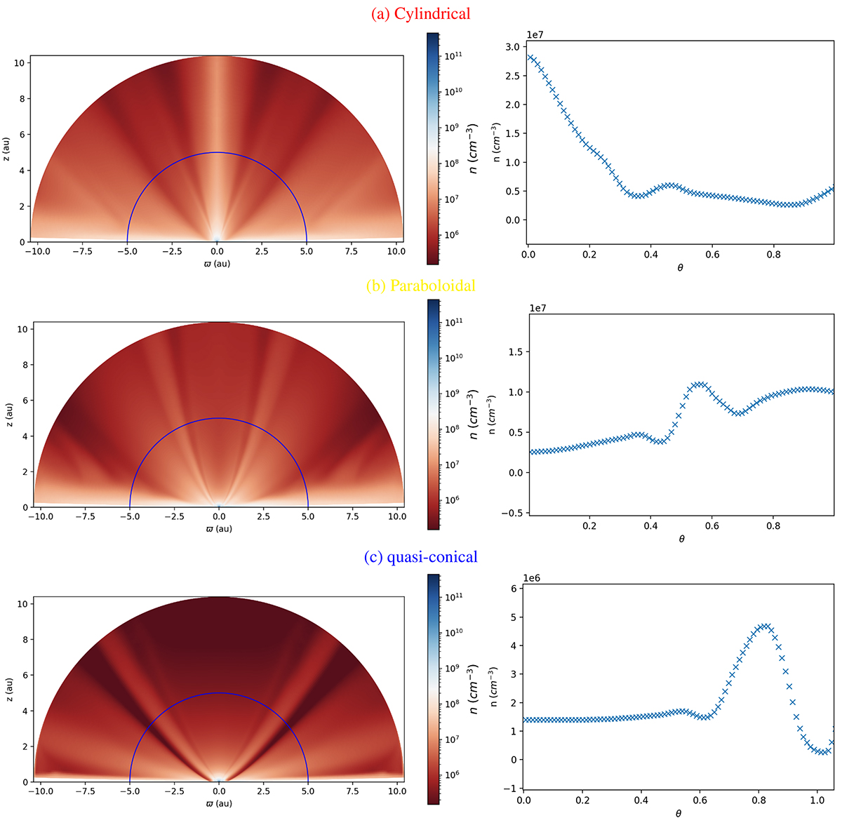
Fig. 6.
Download original image
Plots of jet shapes found in the parameter space. The 2D maps of density show the collimation up to 10 au. What differs between cylindrical and paraboloidal, in this case, is the density at the axis. Generally, the opening angle is sufficient to distinguish cylindrical from paraboloidal solutions. The numerical diffusion is so low that the density isocontours coincide with the magnetic flux tubes and the poloidal velocity line (as in Fig. 9). The more collimated the flow is, the lower the acceleration efficiency. When this does not apply we look at the density distribution on the polar axis. For (a), Rc = 0 au and Ih = 10−1 (R0_I1). Next, for (b), Rc = 0.2 au and Ih = 10−3 (R2_I3). Finally, for (c), Rc = 0.4 au and Ih = 10−3 (R4_I3). The blues half circle on all the cases indicates the radius along which the number density is plotted. We plot the density along θ starting at the axis and stop before reaching the disk wind region.
Current usage metrics show cumulative count of Article Views (full-text article views including HTML views, PDF and ePub downloads, according to the available data) and Abstracts Views on Vision4Press platform.
Data correspond to usage on the plateform after 2015. The current usage metrics is available 48-96 hours after online publication and is updated daily on week days.
Initial download of the metrics may take a while.