| Issue |
A&A
Volume 686, June 2024
|
|
|---|---|---|
| Article Number | A278 | |
| Number of page(s) | 9 | |
| Section | The Sun and the Heliosphere | |
| DOI | https://doi.org/10.1051/0004-6361/202449157 | |
| Published online | 19 June 2024 | |
Forward modeling of the Mg I 12.32 μm line from a 3D magnetohydrodynamic model of an enhanced network
1
National Astronomical Observatories, Chinese Academy of Sciences, Beijing 100101, PR China
e-mail: This email address is being protected from spambots. You need JavaScript enabled to view it.
2
School of Astronomy and Space Science, University of Chinese Academy of Sciences, Beijing 100049, PR China
3
Solar Research Laboratory, National Research Institute of Astronomy and Geophysics Helwan, Cairo 11421, Egypt
4
Key Laboratory of Solar Activity and Space Weather, National Space Science Center, Chinese Academy of Sciences, Beijing 100190, PR China
Received:
4
January
2024
Accepted:
17
April
2024
Abstract
Context. The Mg I 12 μm lines, 12.22 and 12.32 μm, represent a pair of emission lines, and their line cores originate around the temperature minimum region. These lines exhibit the highest ratio of Zeeman to Doppler broadening in the infrared solar spectrum, making them crucial for accurately investigating the solar magnetic field.
Aims. We synthesized the Mg I 12.32 μm Stokes profiles from a 3D magnetohydrodynamic (MHD) model and studied the validity of different methods for extracting the magnetic field. The observational profiles at different spatial resolution were simulated, which are helpful for the design of future solar telescopes with large apertures.
Methods. We used a 3D MHD simulation model for an enhanced network computed using the Bifrost code. We performed nonlocal thermal equilibrium calculations for Stokes profiles of the Mg I 12.32 μm line using the Rybicki–Hummer code.
Results. From the simulation we determined the average formation height of the Mg I 12.32 μm line to be around 450 km. The various solar features have different formation heights, and the variance of formation height in magnetic concentration regions is about 160 km. The wavelength-integrated method is proven effective in calibrating the integrated Stokes profiles to obtain the longitudinal (Bl) and horizontal (BH) field components for weak magnetic fields; the Bl is below 300 G. Furthermore, the weak field approximation was found to be valid only for estimating magnetic fields with Bl below 150 G. The Stokes I profiles clearly show Zeeman triple splitting around the magnetic flux concentration with a grid resolution of 48 km. We determined that a resolution of 0.97″, equivalent to the diffraction limit of a telescope with a diameter of 3.2 m, was necessary to detect the Zeeman splitting for the simulated snapshot. Our results from this 3D MHD model are valuable for interpreting data from the Accurate Infrared Magnetic Field Measurements of the Sun (AIMS) telescope and designing future solar infrared telescopes.
Key words: Sun: atmosphere / Sun: infrared / Sun: magnetic fields
© The Authors 2024
 Open Access article, published by EDP Sciences, under the terms of the Creative Commons Attribution License (https://creativecommons.org/licenses/by/4.0), which permits unrestricted use, distribution, and reproduction in any medium, provided the original work is properly cited.
This article is published in open access under the Subscribe to Open model. This email address is being protected from spambots. You need JavaScript enabled to view it. to support open access publication.
1. Introduction
The Mg I 12 μm emission lines exhibit remarkable properties and a high sensitivity to magnetic fields, making them crucial in solar physics research. These infrared lines are particularly valuable for studying magnetic fields due to their significant ratio of Zeeman split to Doppler broadening; they have the largest Zeeman split observed in the solar spectrum so far. They were first discovered by Murcray et al. (1981) and subsequently identified as transitions between high Rydberg levels of the Mg I atom by Chang & Noyes (1983). Observations of the Mg I 12 μm lines have revealed interesting characteristics. The line profiles of Mg I at 12 μm typically exhibit an emission peak and an absorption trough at the center of the solar disk. However, at the solar limb, the absorption trough disappears and the emission peak becomes more pronounced; they show distinct Zeeman splitting even when subjected to weak magnetic fields (Brault & Noyes 1983). The Mg I 12 μm lines are observed in sunspot penumbrae or plages, while they are absent in sunspot umbrae (Zirin & Popp 1989; Moran et al. 2007; Li et al. 2021). Consequently, they have been utilized to measure total magnetic field strengths in the upper photosphere near the temperature minimum region using infrared Stokes polarimetry (Deming et al. 1988; Hewagama et al. 1993; Moran et al. 2000).
The formation of the Mg I 12 μm lines was investigated by Carlsson & Rutten (1992). They found that these lines originate in the upper photosphere, and the synthesized line profiles matched those of observations when assuming nonlocal thermodynamic equilibrium (NLTE). Furthermore, Bruls et al. (1995) synthesized polarization profiles of these lines and studied their sensitivity to a magnetic field of sunspots and plages. They demonstrated that the Stokes V profiles exhibit wide features that correspond to the absorption trough in the Stokes I profiles. However, recent studies have only synthesized the Mg I 12.32 μm line using 1D atmospheric models (e.g., Hong et al. 2020; Li et al. 2021), and no studies have been performed using 3D atmospheric models. Such studies are important for understanding and interpreting the observations of Mg I 12 μm by the newly developed solar telescopes working in the infrared wavelength, such as the infrared system of the Accurate Infrared Magnetic Field Measurements of the Sun (AIMS; Deng et al. 2016).
The 3D magnetohydrodynamic (MHD) simulation that uses the Bifrost code (Gudiksen et al. 2011) was designed specifically for simulating the dynamic and complex nature of the solar atmosphere. It incorporates a comprehensive set of physical processes and equations to accurately model the behavior of plasma in the solar atmosphere. The code allows for high-resolution simulations, enabling the study of fine-scale structures and dynamics. This spatial resolution is crucial for capturing the intricate details of the magnetic field topology and plasma dynamics. This particular simulation has been used in several studies to synthesize various spectral lines, such as Mg II h & k (Leenaarts et al. 2013), Ca II 8542 Å (Quintero Noda et al. 2016), Lyman β, and O I 1027 & 1028 Å (Hasegawa et al. 2020).
In this study we present the synthesis of the Mg I 12.32 μm line using a 3D MHD simulation obtained from the Bifrost code, which represents a solar enhanced network region. In Sect. 2 we provide a detailed description of the atmospheric and atomic models employed, as well as the numerical radiative transfer code used in our analysis. In Sect. 3 we present the results of our NLTE calculations for the Mg I 12.32 μm line, including the determination of its formation height, and the analysis of some Stokes profiles at various features. We thoroughly investigate the validity of the wavelength-integrated method and the weak field approximation (WFA) for inferring the magnetic field vector. Additionally, we assess the impact of different telescope resolutions on the diagnostic capability of the 12.32 μm line by spatially convolving the synthetic Stokes profiles. Finally, we summarize our results in Sect. 4.
2. Models and methods
2.1. Atmospheric model
We used a 3D MHD simulation computed with the Bifrost code (Gudiksen et al. 2011). The simulation represents an enhanced network region characterized by two opposite magnetic polarities (Carlsson et al. 2016). It comprises a series of snapshots; we specifically selected the 385 snapshot, which corresponds to a simulation time of t = 3850 s. The simulation’s horizontal domain measures 24 × 24 Mm and features a uniform grid spacing of 48 km, composed of 504 × 504 grid cells. In the vertical direction, the simulation spans from the upper convection zone (z = −2.4 Mm) to the corona (z = 14.4 Mm). The height z = 0 corresponds to the average height in the simulation of optical depth unity at 500 nm. The grid spacing is nonuniform in the vertical direction; it is 19 km within the height range −1 Mm < z < 5 Mm and gradually increases to approximately 100 km at the upper boundary. The simulation includes thermal conduction along the magnetic field and assumes optically thick radiative transfer in the photosphere and low chromosphere.
Figure 1 displays horizontal cross sections of temperature (T), longitudinal magnetic field (Bl), and horizontal magnetic field ( ) from the Bifrost snapshot at two different heights (z = 0 km and 450 km). In the first row, which represents the surface (z = 0 km), the temperature distribution has a clear granulation pattern, with wider granules exhibiting higher temperatures compared to the narrower intergranular lanes. The magnetic fields predominantly align vertically and are concentrated within the intergranular lanes as a result of convective motions and the buoyancy of the field. Moving to higher atmospheric heights (second row), we observe a phenomenon known as the reverse granulation pattern: with increasing height, the granules become cooler than the intergranular lanes at the same height. Additionally, the strength of the magnetic field decreases, and its orientation tends to become more horizontal. These changes can be attributed to the reduction in gas pressure and the expansion of the magnetic field in the higher atmosphere.
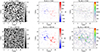 |
Fig. 1. Horizontal cross sections of the temperature (T, left) and the longitudinal (Bl, middle) and horizontal magnetic field strengths (BH, right) at geometrical heights of z = 0 km (top panel) and z = 450 km (bottom panel). Brown dashed lines mark a region that is analyzed later in this paper. |
2.2. Atomic model
We used the atomic model MgI_66.atom, which was derived from the model used in Carlsson & Rutten (1992) and included in the Rybicki–Hummer (RH) package. The energy levels were updated based on the analysis conducted by Kaufman & Martin (1991), and the oscillator strength of the Mg I 12.32 μm line was adjusted to the value reported by Zhao et al. (1998). This atomic model comprises 315 line transitions and 65 bound-free transitions from 66 levels, including the ground level of Mg II. The Mg I 12.32 μm line was initially identified by Chang & Noyes (1983) as a transition between highly excited levels of Mg I 3s7i1, 3I → 3s6h1, 3Ho. The Landé g factor of the Mg I 12.32 μm line, which indicates the line’s sensitivity to the magnetic field, is unity (Chang 1987; Lemoine et al. 1988).
2.3. Synthesis of the Mg I 12.32 μm line
We synthesized the Stokes profiles of the Mg I 12.32 μm line using the RH code (Uitenbroek 2001; Pereira & Uitenbroek 2015) for a line of sight with μ = 1 (μ = cos θ, where θ is the heliocentric angle). The RH code was employed to solve the NLTE radiative transfer problem of the Mg I 12.32 μm line, assuming complete frequency redistribution (CRD) and under the field-free approximation. The NLTE atomic populations were calculated under the assumption of statistical equilibrium at each energy level of the atom, that is to say, assuming an instantaneous balance between all transitions going into and out of each atomic level. The synthesis of Stokes profiles was conducted using the vertical domain of the 3D Bifrost model within the height range z = [ − 0.5, 1.2] Mm. This particular range was chosen due to the sensitivity of the Mg I 12.32 μm line in the photosphere and lower chromosphere, and also to minimize the computational time. Each vertical column of the model was treated as an independent 1D atmosphere, that is, as a plane-parallel atmosphere (referred to as the 1.5D approximation).
3. Results
3.1. Formation height of the Mg I 12.32 μm line in various features
Figure 2 displays the vertical cross sections of the Bifrost atmosphere (i.e., the dashed brown line in Fig. 1). We observed that the Bl (middle panel) exhibited a narrow distribution at the deep photosphere within the flux tubes. However, it expanded in the upper layers of the atmosphere, where the BH component dominated. To determine the formation height, we calculated the height of the optical depth unity for the line core of Mg I 12.32 μm. Remarkably, the formation height varies along the selected slice, particularly in regions where moderate and strong vertical magnetic field patches were present, wherein the formation height reached values of 340 and 160 km, respectively. In these regions, the optical depth shifted toward lower geometrical heights, a phenomenon commonly referred to as Wilson depression. Overall, the average formation height of the Mg I 12.32 μm line was found to be 450 km in the upper photosphere. These findings are consistent with previous studies based on 1D semi-empirical atmospheric models (Carlsson & Rutten 1992; Li et al. 2021).
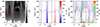 |
Fig. 2. Maps of vertical cuts for the temperature (T; left), the longitudinal field (Bl; middle), and the horizontal field (BH; right). The pixels correspond to the dashed brown line in Fig. 1. The magenta lines mark the heights of optical depth τ = 1 for the line core of Mg I 12.32 μm. Vertical lines correspond to the four atmospheric columns that we studied in detail. |
We studied the properties of the synthetic Stokes I and V profiles obtained from the RH code at different spatial locations. In Fig. 2 we can identify four pixels that correspond to the vertical lines and represent two magnetic concentrations (that include strong and moderate field strengths), the border of a magnetic concentration, and a weak field region. Figure 3 displays the synthetic Stokes I and V profiles, along with the vertical stratification of the temperature and the magnetic field strength, for these four selected pixels. Each row corresponds to a different pixel.
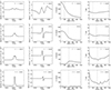 |
Fig. 3. Synthetic Stokes I (first column) and Stokes V profiles (second column), and the corresponding vertical stratification of the magnetic field strength (B; third column) and temperature (T; fourth column) for the four vertical atmospheric columns (in Fig. 2 the line style at the top of each panel indicates the corresponding atmosphere). The vertical dotted line in third and fourth columns indicates the corresponding formation height at optical depth τ = 1, as show in Fig. 2. |
In the first and second rows, which represent the centers of the magnetic concentrations, the intensity profiles clearly exhibit Zeeman splitting. The strong magnetic concentration (first row) displays greater Stokes I splitting compared to the relatively weak one (second row). Additionally, the line profile in the first row is broader than in the second, and this distinction can be attributed to two factors. Firstly, the formation of the Mg I 12.32 μm line occurs at a lower height within the center of the strong magnetic concentration. Secondly, the temperature gradient in the first row is shallower. The third row shows the Stokes I profile for a region located at the border of the magnetic concentration, where the magnetic field becomes more horizontal (as shown in the right panel of Fig. 2). The Stokes I profile exhibits two σ components and one π component, along with evident absorption troughs. However, the synthetic Stokes I profiles at the center and border of the magnetic concentrations agree with observations of strong solar features (Hewagama et al. 1993; Zirin & Popp 1989; Moran et al. 2000). In the weak field region (fourth column), the Stokes I profile has an emission peak accompanied by wide absorption troughs, consistent with observations of quiet-Sun regions (Brault & Noyes 1983; Zirin & Popp 1989) and numerical calculations based on semi-empirical atmospheric models (Carlsson & Rutten 1992; Zhao et al. 1998; Li et al. 2021). Interestingly, we note that the Stokes I profiles within the magnetic concentrations exhibit the highest continuum intensity, and we see intensity brightening near the magnetic concentration regions (bright points), as seen in the left panel of Fig. 4.
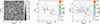 |
Fig. 4. Maps of integrated intensity (left), MCPD (middle), and MLPD (right) for the synthetic profiles of the Mg I 12.32 μm line. |
The second column of Fig. 3 demonstrates that the synthetic Stokes V profiles exhibit distinct splitting and absorption trough features, which become less apparent as the magnetic field weakens. Interestingly, a few Stokes V profiles in our calculations have four lobes, primarily located at the center of strong magnetic concentrations, as depicted in the first row of the second column. This profile shape has previously been found in solar flares through both observations (Jennings et al. 2002) and simulations (Hong et al. 2020). Furthermore, we notice that the Mg I 12.32 μm line is predominantly formed at heights near the temperature minimum, as clearly evidenced by the vertical temperature stratification in the fourth column of Fig. 3.
3.2. Integrated Stokes profiles
We integrated the synthetic Stokes profiles and calculated the mean circular polarization degree (MCPD) and mean linear polarization degree (MLPD), which were described by Sainz Dalda et al. (2012) as follows:
 (1)
(1)
 (2)
(2)
where the numerical integration is performed from λa = 12 315.182 nm to λb = 12 321.169 nm. The MCPD and MLPD are related to the Bl and BH, respectively. They serve as effective tools for diagnosing the strength of the magnetic field at the formation height of the spectral line. The maps of the integrated intensity, MCPD, and MLPD are presented in Fig. 4. By comparing the second row in Fig. 1 with Fig. 4, it becomes evident that the integrated intensity map closely reflects the temperature distribution at a geometrical height of z = 450 km, that is to say, it shows a reverse granulation pattern, wherein the regions of granules appear cooler than the intergranular lanes. The primary distinction between the two maps lies in the presence of bright points within the integrated polarization map, which correspond to magnetic flux concentrations exhibiting a strong vertical magnetic field (see the second row of the middle panel in Fig. 1). Furthermore, the maps of MCPD and MLPD exhibit a significant correlation with the Bl and BH components, respectively, at a geometrical height of z = 450 km. The regions with the highest MCPD values are located in the inner parts of strong magnetic flux concentrations, which correspond to regions of strong vertical magnetic fields. On the other hand, the regions with the highest MLPD values are found at the borders of flux concentrations, where the magnetic field lines are inclined and spread more out of the flux tube with increasing height. These results provide conclusive evidence that the formation height of the Mg I 12.32 μm line is located within the height range of 450 km for the Bifrost simulation.
Figure 5 shows the relation between the MCPD and Bl (top panel) and between the MLPD and BH (bottom panel), as derived from the simulation model at a geometrical height of z = 450 km. These relations can be considered a conversion of the MCPD (MLPD) to Bl (BH). A linear relation correlation is found between the MCPD and Bl within the Bl range of 0−300 G, whereas the MLPD and BH exhibited linearity across the entire range of BH (0−325 G). Regarding the MCPD and Bl, the scatter plots show a larger dispersion for Bl values greater than 150 G, indicating that the linear calibration method has a larger error due to the fact that the WFA is not validated. These findings are consistent with the results obtained by Li et al. (2021) using a 1D model atmosphere. Li et al. (2021) suggest that the wavelength-integrated method is suitable for calibrating Bl and BH in the case of linear calibration, where Bl < 300 G and BH < 500. However, due to limitations in our simulation model, the strongest BH is 325 G at the formation height of 450 km. Therefore, we were unable to determine the saturation limit of BH using this method.
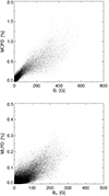 |
Fig. 5. Scatter plots of MCPD (top panel) and MLPD (bottom panel) as a function of the Bl and BH of the simulation model, respectively, at a height of 450 km. |
3.3. Validity of the weak field approximation
When the Zeeman splitting (ΔλB) of the spectral line is significantly smaller than the typical line width (ΔλD), the WFA method can be be employed to determine the line-of-sight component of the magnetic field vector (BLOS). By analyzing the Stokes I and V profiles, the value of BLOS can be computed following Martínez González & Bellot Rubio (2009) and Centeno (2018):
 (3)
(3)
where the constant, C, is determined by the effective Landé factor ( ) and the central wavelength (λo) of the spectral line as
  . The syntheses of the spectral profiles were performed at disk center (μ = 1), so BLOS = Bl. We used the entire range of wavelengths along the Stokes profiles, ranging from 12 315.182 nm to 12 321.169 nm. Figure 6 illustrates the Bl derived from the WFA (top panel) and the actual field in the MHD simulation at a height of 450 km (bottom panel). We find significant similarities between the two maps of the longitudinal magnetic field (Bl) obtained from the WFA and the actual field in the simulation. Furthermore, we compared the values of Bl in the simulation model with those computed using the WFA, as shown in Fig. 7. The WFA values are more accurate and closely match those of the model for Bl < 150 G. This result is consistent with the relationship between the MCPD and Bl shown in Fig. 5. This analysis demonstrates that the WFA method is useful for understanding and interpreting the observations of AIMS and future mid-infrared solar telescopes of quiet-Sun regions.
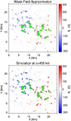 |
Fig. 6. Maps of Bl as derived from the WFA method (top panel) and MHD simulation at a height of 450 km (bottom panel). Green regions mark the excluded pixels whose Stokes I profiles exhibit Zeeman splitting. |
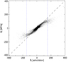 |
Fig. 7. Bl as inferred from the WFA versus the actual values in the MHD simulation model. Vertical dotted blue lines demarcate the region of validity of the WFA (see the main text). |
3.4. The effect of spatial resolution
In observations, the aperture of a telescope is limited. The largest solar telescope in China taking routine observations is 1 m, and the largest solar telescope globally, the Daniel K. Inouye Solar Telescope (DKIST), has a 4 m aperture (Rimmele et al. 2020). In other words, the spatial resolution of existing solar telescopes is limited. As the Mg I 12.32 μm wavelength is in the mid-infrared, the diffraction limit resolution is much lower than that for the visible wavelength. The simulation has a pixel size of 48 km (equivalent to  ), which implies a spatial resolution of
  . For AIMS with a 1 m aperture, the diffraction limit is about 3 arcsec (about 2175 km in the Sun) at 12.32 μm, much lower than the grid size of the Bifrost simulation. Keeping these considerations in mind, we convolved the maps of synthetic Stokes profiles with Gaussian functions of different full widths at half maximum (FWHMs) to simulate the point spread function (PSF) of a telescope and study the effect of spatial resolution. The FWHM was calculated according to the Rayleigh criterion FWHM = 1.22λ/D. Therefore,
 (4)
(4)
where D is the aperture diameter expressed in meters, λ is the wavelength in meters, and the FWHM is in arcseconds. The PSF was determined mainly according to the aperture of three solar telescopes: the 1 m AIMS infrared system (Deng et al. 2016), the 4 m DKIST (Rimmele et al. 2020), and the proposed 8 m Chinese Giant Solar Telescope (CGST; Liu et al. 2012). They have spatial resolutions of  ,
,  , and
, and  , respectively. Figure 8 displays the maps of the MCPD and MLPD for the spatially degraded Stokes profiles, taking the different telescope diffraction limits into account. A comparison between Figs. 4 and 8 reveals that increasing the degraded resolution leads to a decrease in the magnitudes of the MCPD and MLPD at the simulation resolution of
  . The peak magnitudes of the MCPD (MLPD) are 4.6 (0.56), 1.2 (0.25), 0.9 (0.16), and 0.3 (0.03) at spatial resolutions of
  ,
,  ,
,  , and
, and  , respectively. Furthermore, the maps appear more blurred, and an increasing number of atmospheric fine structures disappear because of the decrease in resolution with a wider PSF.
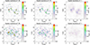 |
Fig. 8. Maps of MCPD (first row) and MLPD (second row) for the degraded profiles of the Mg I 12.32 μm line at spatial resolutions of |


We selected a pixel located at the center of a strong magnetic flux concentration to show the effect of spatial resolution in detail. The Stokes I and V profiles of this pixel, obtained at the simulation resolution and three additional degraded resolutions, are displayed in Fig. 9. At the simulation resolution  , the Stokes I profile clearly exhibits Zeeman splitting in the emission peak, characterized by wide absorption troughs and a large line width. The Stokes V profile has a complex shape, with four lobes. As we decrease the spatial resolution, the Zeeman splitting in the Stokes I profile decreases, and the two σ components become closer to each other. Furthermore, the amplitudes of the Stokes V lobes decrease, and the splitting becomes smaller. However, at a spatial resolution of
  , the Stokes I profile does not show Zeeman splitting, and the absorption trough feature disappears. Additionally, the Stokes V profile shows a normal shape with two lobes as well as two wider features at the edges.
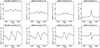 |
Fig. 9. Synthetic Stokes I (first row) and Stokes V profiles (second row), corresponding to a simulation resolution of |


We used a total of 504 × 504 synthetic Stokes I profiles calculated from the Bifrost simulation to determine the necessary spatial resolution for observing Zeeman splitting. Interestingly, 2.4% of Stokes I profiles (i.e., 6027) exhibit distinct Zeeman splitting. Figure 10 shows the required spatial resolution for detecting this specific portion of the Stokes I profiles with distinct splitting as observed in the simulation. The percent of Stokes I profiles decreases with the spatial resolution of a telescope. Additionally, we depict the telescope diameter necessary for achieving this spatial resolution, as determined by Eq. (4). From this snapshot of a network region, our results indicate that a telescope with a diameter of 7.2 m and a spatial resolution of  can detect 50% of the simulated Stokes I splitting. Furthermore, 5% of the Stokes I splitting can be observed by a telescope with a diameter of 3.2 m and a spatial resolution of
  , which is the minimum resolution required for detecting Zeeman splitting. The results obtained from this investigation on spatial resolution can inform the specifications of future solar telescopes intended for observing the Mg I 12.32 μm line.
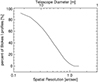 |
Fig. 10. Percent of Stokes I profiles with clear Zeeman splitting as a function of the spatial resolution and the telescope diameter that yields the spatial resolution, as indicated at the top of the plot. |
4. Conclusions and discussion
We employed the RH code to synthesize the Mg I 12.32 μm line using a 3D MHD simulation model. The atmospheric model utilized in this study was obtained from the Bifrost code, which represents an enhanced network region. We performed column-by-column computations assuming a plane-parallel atmosphere. The NLTE calculations were conducted assuming CRD.
A specific slice from the MHD simulation containing a few magnetic flux concentrations was selected. By calculating the height of the optical depth unity for the line core of Mg I 12.32 μm along this slice, we determined the formation height, which was found to be in the upper photosphere at approximately 450 km above the solar surface. Furthermore, we examined the polarimetric profiles of the Mg I 12.32 μm line in various features. The Stokes I profiles originating from the magnetic flux concentrations and its border displayed clear Zeeman splitting and wide absorption troughs, and its formation heights are 160 km and 340 km, which are lower than the other features. In regions with weak magnetic fields, the Stokes I profiles exhibit an emission peak, consistent with previous observations of the quiet Sun. Moreover, the Stokes V profiles exhibit two lobes with extended wide features at the wings, while a complex Stokes V profile with four lobes was observed at the center of a strong magnetic flux concentration.
The synthetic Stokes profiles were integrated, and we computed the MCPD and MLPD. Notably, the spatial distributions of integrated intensity, the MCPD, and the MLPD show a strong correlation with the temperature, Bl, and BH distributions, respectively, at the geometrical height of 450 km in the simulation. These findings align with the results obtained from our calculations for the height of the optical depth unity for the line core of Mg I 12.32 μm. Furthermore, we expanded upon these results by investigating the applicability of the wavelength-integrated method and the WFA as convenient and rapid tools for estimating the line-of-sight and perpendicular components of the magnetic field strength from the Stokes profiles. Using the wavelength-integrated method, we observed a linear relation between the Bl and MCPD within the range 0 G < Bl < 300 G, and between BH and MLPD within the entire BH range; this relation determines the saturation of the method.
Additionally, we find that the WFA can successfully extract the Bl component from the synthetic profiles when the magnetic field is weak (i.e., a Bl below 150 G) and the Zeeman splitting of Mg I 12.32 μm is significantly smaller than the line width. However, the wavelength-integrated method and the WFA provide estimations for weak magnetic fields under the assumption that the fields are fully resolved (i.e., the filling factor f = 1). Therefore, the resulting magnetic field strengths should be considered approximate values. For accurate field strength measurements, especially for the regions where the WFA does not work, it is necessary to use Stokes inversion codes that account for line formation under NLTE conditions, such as NICOLE (Socas-Navarro et al. 2015), STIC (de la Cruz Rodríguez et al. 2019), and DeSIRe (Ruiz Cobo et al. 2022). This aspect of the study will be addressed in future research.
We degraded the synthetic Stokes maps according to the apertures of AIMS, DKIST, and CGST to investigate the spatial resolution. At the spatial resolutions of DKIST and CGST, some of the Stokes I profiles still exhibited Zeeman splitting, with the two σ components becoming closer to each other as the resolution decreased. A few Stokes V profiles displayed a complex four-lobe structure. However, at the resolution of AIMS, we were unable to detect any Zeeman splitting in the Stokes I profiles for our used snapshot. We find that a resolution of  , corresponding to a telescope with a diameter of 3.2 m, was necessary to detect the Zeeman splitting of the magnetic concentration region or bright points in the quiet-Sun regions.
This analysis is based on the synthetic profiles of Mg I 12.32 μm obtained by the RH code using a 3D MHD simulation of an enhanced network. Our results demonstrate that the Mg I 12.32 μm line is a valuable tool for accurately determining the magnetic field strength in the upper photosphere thanks to its high sensitivity. Specifically, 2.4% of Stokes I profiles exhibit distinct Zeeman splitting, and complex Stokes V profiles with four lobes were found in regions with strong vertical magnetic fields. To gain further insight and improve the interpretation of future observations, more studies that employ 3D MHD simulations are needed to explore the behavior of the Mg I 12.32 μm line in other solar features, such as sunspot models (Rempel & Cheung 2014; Chen et al. 2017; Panja et al. 2021; Danilovic 2023).
Acknowledgments
This research work is supported by the National Key R & D Program of China (2021YFA1600500), the Youth Innovation Promotion Association CAS (2023061) and the National Natural Science Foundation of China (NSFC, Grant Nos. 12003051, 12373058 and 11427901).
References
- Brault, J., & Noyes, R. 1983, ApJ, 269, L61 [Google Scholar]
- Bruls, J. H. M. J., Solanki, S. K., Rutten, R. J., & Carlsson, M. 1995, A&A, 293, 225 [NASA ADS] [Google Scholar]
- Carlsson, M., & Rutten, R. J. 1992, A&A, 259, L53 [NASA ADS] [Google Scholar]
- Carlsson, M., Hansteen, V. H., Gudiksen, B. V., Leenaarts, J., & De Pontieu, B. 2016, A&A, 585, A4 [NASA ADS] [CrossRef] [EDP Sciences] [Google Scholar]
- Centeno, R. 2018, ApJ, 866, 89 [Google Scholar]
- Chang, E. S. 1987, Phys. Scr., 35, 792 [Google Scholar]
- Chang, E. S., & Noyes, R. W. 1983, ApJ, 275, L11 [Google Scholar]
- Chen, F., Rempel, M., & Fan, Y. 2017, ApJ, 846, 149 [Google Scholar]
- Danilovic, S. 2023, Adv. Space Res., 71, 1939 [NASA ADS] [CrossRef] [Google Scholar]
- de la Cruz Rodríguez, J., Leenaarts, J., Danilovic, S., & Uitenbroek, H. 2019, A&A, 623, A74 [Google Scholar]
- Deming, D., Boyle, R. J., Jennings, D. E., & Wiedemann, G. 1988, ApJ, 333, 978 [Google Scholar]
- Deng, Y., Liu, Z., Qu, Z., Liu, Y., & Ji, H. 2016, in Coimbra Solar Physics Meeting: Ground-based Solar Observations in the Space Instrumentation Era, eds. I. Dorotovic, C. E. Fischer, & M. Temmer, ASP Conf. Ser., 504, 293 [Google Scholar]
- Gudiksen, B. V., Carlsson, M., Hansteen, V. H., et al. 2011, A&A, 531, A154 [NASA ADS] [CrossRef] [EDP Sciences] [Google Scholar]
- Hasegawa, T., Noda, C. Q., Shimizu, T., & Carlsson, M. 2020, ApJ, 900, 34 [CrossRef] [Google Scholar]
- Hewagama, T., Deming, D., Jennings, D. E., et al. 1993, ApJS, 86, 313 [Google Scholar]
- Hong, J., Bai, X., Li, Y., Ding, M. D., & Deng, Y. 2020, ApJ, 898, 134 [Google Scholar]
- Jennings, D. E., Deming, D., McCabe, G., Sada, P. V., & Moran, T. 2002, ApJ, 568, 1043 [NASA ADS] [CrossRef] [Google Scholar]
- Kaufman, V., & Martin, W. C. 1991, J. Phys. Chem. Ref. Data, 20, 83 [NASA ADS] [CrossRef] [Google Scholar]
- Leenaarts, J., Pereira, T. M. D., Carlsson, M., Uitenbroek, H., & De Pontieu, B. 2013, ApJ, 772, 90 [NASA ADS] [CrossRef] [Google Scholar]
- Lemoine, B., Demuynck, C., & Destombes, J. L. 1988, A&A, 191, L4 [Google Scholar]
- Li, X., Song, Y., Uitenbroek, H., et al. 2021, A&A, 646, A79 [NASA ADS] [CrossRef] [EDP Sciences] [Google Scholar]
- Liu, Z., Deng, Y., Jin, Z., & Ji, H. 2012, in Ground-based and Airborne Telescopes IV, eds. L. M. Stepp, R. Gilmozzi, & H. J. Hall, SPIE Conf. Ser., 8444, 844405 [NASA ADS] [CrossRef] [Google Scholar]
- Martínez González, M. J., & Bellot Rubio, L. R. 2009, ApJ, 700, 1391 [CrossRef] [Google Scholar]
- Moran, T., Deming, D., Jennings, D. E., & McCabe, G. 2000, ApJ, 533, 1035 [NASA ADS] [CrossRef] [Google Scholar]
- Moran, T. G., Jennings, D. E., Deming, L. D., et al. 2007, Sol. Phys., 241, 213 [NASA ADS] [CrossRef] [Google Scholar]
- Murcray, F. J., Goldman, A., Murcray, F. H., et al. 1981, ApJ, 247, L97 [Google Scholar]
- Panja, M., Cameron, R. H., & Solanki, S. K. 2021, ApJ, 907, 102 [Google Scholar]
- Pereira, T. M. D., & Uitenbroek, H. 2015, A&A, 574, A3 [NASA ADS] [CrossRef] [EDP Sciences] [Google Scholar]
- Quintero Noda, C., Shimizu, T., de la Cruz Rodríguez, J., et al. 2016, MNRAS, 459, 3363 [Google Scholar]
- Rempel, M., & Cheung, M. C. M. 2014, ApJ, 785, 90 [Google Scholar]
- Rimmele, T. R., Warner, M., Keil, S. L., et al. 2020, Sol. Phys., 295, 172 [Google Scholar]
- Ruiz Cobo, B., Quintero Noda, C., Gafeira, R., et al. 2022, A&A, 660, A37 [NASA ADS] [CrossRef] [EDP Sciences] [Google Scholar]
- Sainz Dalda, A., Martínez-Sykora, J., Bellot Rubio, L., & Title, A. 2012, ApJ, 748, 38 [NASA ADS] [CrossRef] [Google Scholar]
- Socas-Navarro, H., de la Cruz Rodríguez, J., Asensio Ramos, A., Trujillo Bueno, J., & Ruiz Cobo, B. 2015, A&A, 577, A7 [NASA ADS] [CrossRef] [EDP Sciences] [Google Scholar]
- Uitenbroek, H. 2001, ApJ, 557, 389 [Google Scholar]
- Zhao, G., Butler, K., & Gehren, T. 1998, A&A, 333, 219 [NASA ADS] [Google Scholar]
- Zirin, H., & Popp, B. 1989, ApJ, 340, 571 [NASA ADS] [CrossRef] [Google Scholar]
All Figures
|
Fig. 1. Horizontal cross sections of the temperature (T, left) and the longitudinal (Bl, middle) and horizontal magnetic field strengths (BH, right) at geometrical heights of z = 0 km (top panel) and z = 450 km (bottom panel). Brown dashed lines mark a region that is analyzed later in this paper. |
| In the text | |
|
Fig. 2. Maps of vertical cuts for the temperature (T; left), the longitudinal field (Bl; middle), and the horizontal field (BH; right). The pixels correspond to the dashed brown line in Fig. 1. The magenta lines mark the heights of optical depth τ = 1 for the line core of Mg I 12.32 μm. Vertical lines correspond to the four atmospheric columns that we studied in detail. |
| In the text | |
|
Fig. 3. Synthetic Stokes I (first column) and Stokes V profiles (second column), and the corresponding vertical stratification of the magnetic field strength (B; third column) and temperature (T; fourth column) for the four vertical atmospheric columns (in Fig. 2 the line style at the top of each panel indicates the corresponding atmosphere). The vertical dotted line in third and fourth columns indicates the corresponding formation height at optical depth τ = 1, as show in Fig. 2. |
| In the text | |
|
Fig. 4. Maps of integrated intensity (left), MCPD (middle), and MLPD (right) for the synthetic profiles of the Mg I 12.32 μm line. |
| In the text | |
|
Fig. 5. Scatter plots of MCPD (top panel) and MLPD (bottom panel) as a function of the Bl and BH of the simulation model, respectively, at a height of 450 km. |
| In the text | |
|
Fig. 6. Maps of Bl as derived from the WFA method (top panel) and MHD simulation at a height of 450 km (bottom panel). Green regions mark the excluded pixels whose Stokes I profiles exhibit Zeeman splitting. |
| In the text | |
|
Fig. 7. Bl as inferred from the WFA versus the actual values in the MHD simulation model. Vertical dotted blue lines demarcate the region of validity of the WFA (see the main text). |
| In the text | |
|
Fig. 8. Maps of MCPD (first row) and MLPD (second row) for the degraded profiles of the Mg I 12.32 μm line at spatial resolutions of |
| In the text | |
|
Fig. 9. Synthetic Stokes I (first row) and Stokes V profiles (second row), corresponding to a simulation resolution of |
| In the text | |
|
Fig. 10. Percent of Stokes I profiles with clear Zeeman splitting as a function of the spatial resolution and the telescope diameter that yields the spatial resolution, as indicated at the top of the plot. |
| In the text | |
Current usage metrics show cumulative count of Article Views (full-text article views including HTML views, PDF and ePub downloads, according to the available data) and Abstracts Views on Vision4Press platform.
Data correspond to usage on the plateform after 2015. The current usage metrics is available 48-96 hours after online publication and is updated daily on week days.
Initial download of the metrics may take a while.