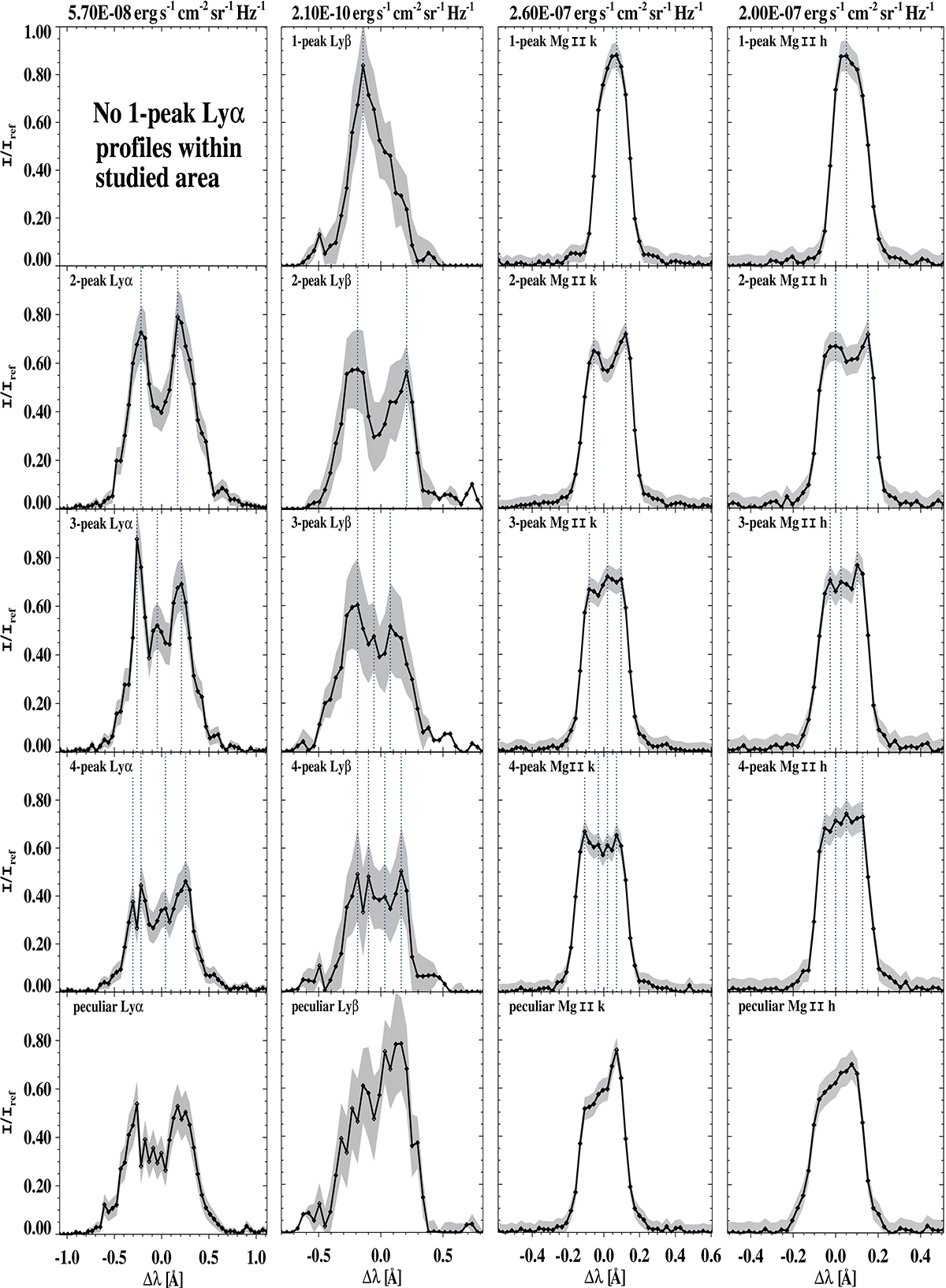
Fig. 7.
Download original image
Examples of different types of spectral line profiles according to the number of peaks detected regardless of the noise (as in colored maps shown in the columns on the left in Figs. 5 and 6). In columns from the left, spectral profiles of Lyα, Lyβ, Mg II k, and Mg II h are shown. In rows from the top, plots of 1-, 2-, 3-, 4-peak and peculiar profiles are located. Error margins of intensities are shown as gray areas around plot-lines. On abscissas, relative wavelength scales Δλ = λ − λ0 are used (for the λ0 values see Table 1). The relative intensities I/Iref are on ordinates; intensities Iref in erg s−1 cm−2 sr−1 Hz−1 are shown at the top of each column for individual spectral lines. The positions of all peaks are marked with blue vertical dotted lines. For a given type of profile (row of the figure) the Lyman line profiles are not from the same position nor from the same time while Mg II k and h profiles of given type are.
Current usage metrics show cumulative count of Article Views (full-text article views including HTML views, PDF and ePub downloads, according to the available data) and Abstracts Views on Vision4Press platform.
Data correspond to usage on the plateform after 2015. The current usage metrics is available 48-96 hours after online publication and is updated daily on week days.
Initial download of the metrics may take a while.