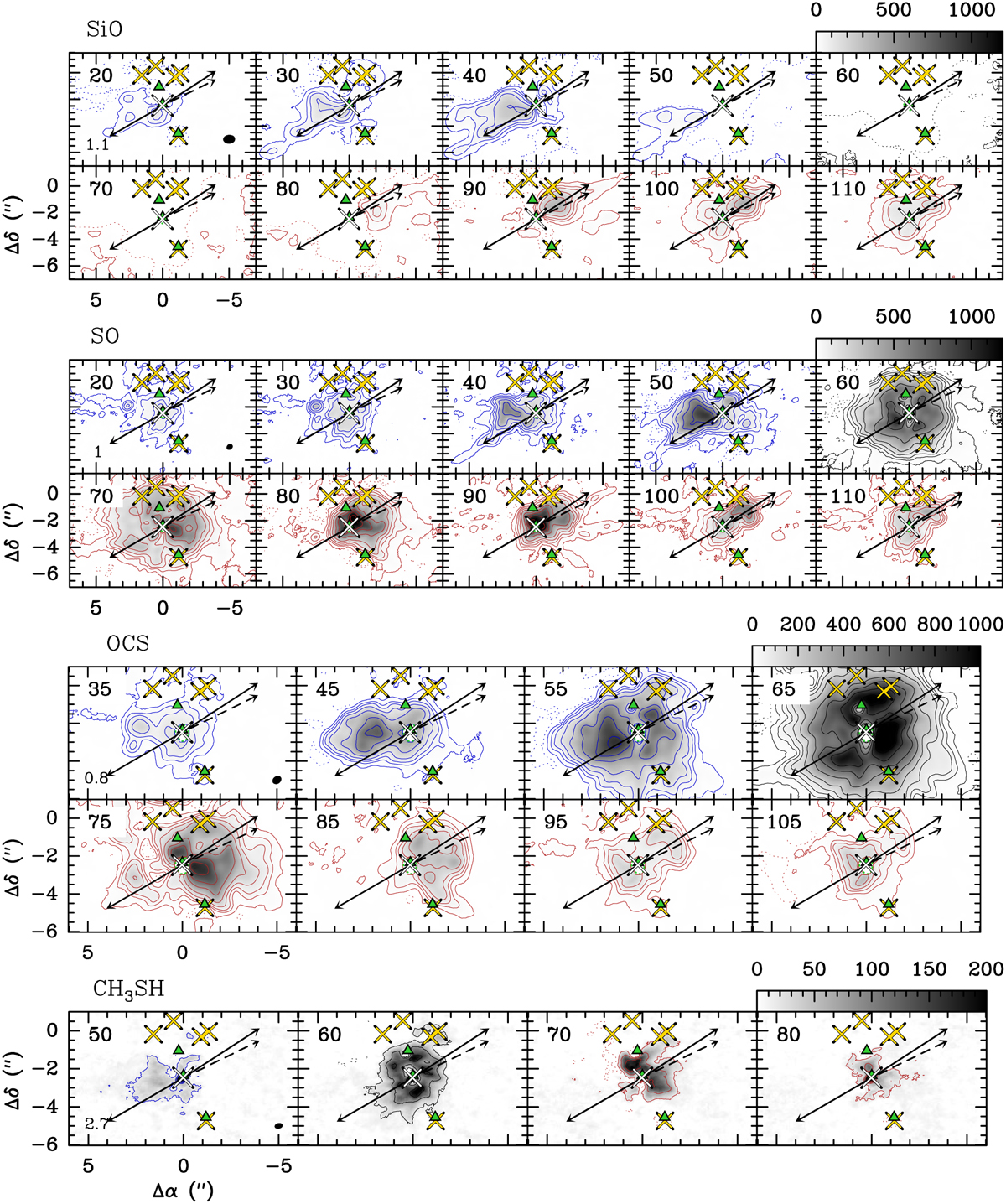
Velocity-channel maps of various molecules (in grey scale (K km s⁻¹) and contours). The integration strategy is the same as for the maps in Figs. 4 and C.1-C.3 (i.e. using two transitions to minimise contamination by other molecules, except for SiO and SO (109.25 GHz)), but in each panel the intensities were integrated over an interval of only 10 km s⁻¹. The respective central velocity in km s⁻¹ is shown in the top left corner. The start and end velocities correspond to the outer integration limits used in Fig. 4. For all molecules but SO, the contours are −6σ, 6σ, 30σ, and then increase by a factor of 2, where σ in K km s⁻¹ is written in the bottom left corner of the lowest-velocity map and was computed using , where N is the number of channels that was integrated over, rms was taken from Table 2 in Belloche et al. (2019), and ∆t; is the channel separation in km s⁻¹. The SO contours start at 10σ and then increase by a factor of 3. Blue contours indicate blue-shifted emission, red contours red-shifted emission, and black contours emission close to the source systemic velocity. Masked regions, arrows, and markers are the same as in Fig. 2. The HPBW is shown in the bottom right corner of the lowest-velocity panel.