| Issue |
A&A
Volume 679, November 2023
|
|
|---|---|---|
| Article Number | A77 | |
| Number of page(s) | 7 | |
| Section | Extragalactic astronomy | |
| DOI | https://doi.org/10.1051/0004-6361/202347172 | |
| Published online | 10 November 2023 | |
Are there more galaxies than we see around high-z quasars?
1
Scuola Normale Superiore, Piazza dei Cavalieri 7, 56126 Pisa, Italy
2
Dipartimento di Fisica, Sapienza, Università di Roma, Piazzale Aldo Moro 5, 00185 Roma, Italy
e-mail: This email address is being protected from spambots. You need JavaScript enabled to view it.
3
INAF – Osservatorio Astronomico di Bologna, Via Piero Gobetti 93/3, 40129 Bologna, Italy
4
INAF – Osservatorio Astronomico di Capodimonte, Via Moiariello 16, 30131 Napoli, Italy
Received:
13
June
2023
Accepted:
6
September
2023
Abstract
Context. It is still debated whether z ≳ 6 quasars lie in the most massive dark matter haloes of the Universe. While most theoretical studies support this scenario, current observations yield discordant results when they probe the halo mass through the detection rate of quasar companion galaxies. Feedback processes from supermassive black holes and dust obscuration have been blamed for this discrepancy, but these effects are complex and far from being clearly understood.
Aim. This paper aims to improve the interpretation of current far-infrared observations by taking the cosmological volume probed by the Atacama Large Millimeter/submillimeter Array Telescope into account and to explain the observational discrepancies.
Methods. We statistically investigated the detection rate of quasar companions in current observations and verified whether they match the expected distribution from various theoretical models when they are convolved with the ALMA field of view through the use of Monte Carlo simulations.
Results. We demonstrate that the telescope geometrical bias is fundamental and can alone explain the scatter in the number of detected satellite galaxies in different observations. We conclude that the resulting companion densities depend on the chosen galaxy distributions. According to our fiducial models, current data favour a density scenario in which quasars lie in dark matter haloes with a viral mass of Mvir ≳ 1012 M⊙, in agreement with most theoretical studies. According to our analysis, each quasar has about two companion galaxies, with a [CII] luminosity L[CII] ≳ 108 L⊙, within a distance of about 1 Mpc from the quasar.
Key words: methods: statistical / methods: numerical / galaxies: high-redshift / galaxies: halos / infrared: galaxies / quasars: general
© The Authors 2023
 Open Access article, published by EDP Sciences, under the terms of the Creative Commons Attribution License (https://creativecommons.org/licenses/by/4.0), which permits unrestricted use, distribution, and reproduction in any medium, provided the original work is properly cited.
This article is published in open access under the Subscribe to Open model. This email address is being protected from spambots. You need JavaScript enabled to view it. to support open access publication.
1. Introduction
Most luminous (Lbol > 1046 erg s−1) quasars at redshift z ≳ 6 are powered by the accretion process of gas onto the most massive supermassive black holes (108 − 1010 M⊙; Ferrarese & Ford 2005; Meyer et al. 2022; Wang et al. 2018). According to theoretical models, including numerical simulations (Sijacki et al. 2009; Di Matteo et al. 2012; Costa et al. 2014; Weinberger et al. 2018; Barai et al. 2018; Habouzit et al. 2019; Ni et al. 2020; Valentini et al. 2021) and clustering studies (Hickox et al. 2009; Ross et al. 2009; Cappelluti et al. 2010; Allevato et al. 2011, 2012), supermassive black holes reside in the densest regions of the Universe, such as the centre of most massive dark matter haloes, with virial masses ranging from 1012 to 1013 M⊙ at z ∼ 6.
However, observations do not always agree with these studies at nearly any redshift. Numerous observational works have exploited current astronomical facilities to investigate the properties of the environments in which quasars reside and yielded differing results. On the one hand, some studies suggested that quasars are located in regions that are characterized by high densities of galaxies, such as Steidel et al. (2005) at z = 2.3, Hall et al. (2018) at 0.5 ≲ z ≲ 3.5, Swinbank et al. (2012) at 2.2 ≲ z ≲ 4.5, García-Vergara et al. (2019); Uchiyama et al. (2020) at z ∼ 4, Husband et al. (2013) and Capak et al. (2011) at z ∼ 5, and Kim et al. (2009); Morselli et al. (2014); Balmaverde et al. (2017); Decarli et al. (2017); Decarli et al. (2018); Mignoli et al. (2020); Venemans et al. (2020) at z ≳ 6. On the other hand, some works, such as Francis & Bland-Hawthorn (2004) and Simpson et al. (2014) at z ≳ 2, Uchiyama et al. (2018) at z ∼ 4, Kashikawa et al. (2007) and Kikuta et al. (2017) at z ∼ 5, and Bañados et al. (2013); Mazzucchelli et al. (2017); Champagne et al. (2018); Meyer et al. (2022) at z ≳ 6, reported that the number of companion galaxies is at most similar to the galaxy density estimated in blank fields. Overall, the question of whether quasars tend to live in over-dense regions of the Universe remains an active area of research.
The detection of Lyman-break galaxies (LBGs) and Lyman-alpha emitting galaxies (LAEs) in the neighbourhoods of quasars and active galactic nuclei is often used in the literature to probe the underlying dark matter distribution of high-redshift structures (see e.g., Intema et al. 2006; Venemans et al. 2007; Bañados et al. 2013; Hennawi et al. 2015; Mazzucchelli et al. 2017, investigating the satellite number counts, or García-Vergara et al. 2019, studying the cross correlation between galaxies and quasars). The contradictory conclusions of these studies may also stem from the intrinsic challenges in constraining the redshift of LBGs and the significant influence of dust extinction and obscuration on both LBGs and LAEs. For this reason, the best strategy for detecting high-z quasar companions relies on the observation of their [CII]158 μm emission as this gas tracer is not affected by dust attenuation and absorption from the intergalactic medium (e.g., Maiolino et al. 2005; Walter et al. 2009). In this context, the Atacama Large Millimeter Array (ALMA) has provided the most numerous spectroscopically confirmed detections of z ≳ 6 quasar companions (Decarli et al. 2017, 2018; Venemans et al. 2020). In particular, Venemans et al. (2020, hereafter V20) found 27 line-emitter candidates within 27 quasar fields. Out of this initial pool, 10 line emitters were already recognised as quasar companions in previous works (Decarli et al. 2017; Willott et al. 2017; Neeleman et al. 2019; Venemans et al. 2019). The remaining candidates have been identified as companions by assuming that the detected line does correspond to the carbon [CII] transition, which is emitted within ±Δv from the quasar. In this work, we assume that the hypothesis of V20 is valid and therefore consider all the additional 17 line emitters as proper quasar companions. Two thresholds were adopted in V20 leading to slightly different results: Seven additional satellites are detected with Δv = 1000 km s−1, and nine satellites with Δv = 2000 km s−1. The V20 sample currently is the largest and most complete catalogue of high-z quasar companions with constrained redshifts.
One debated possibility to explain the differences among these observational results is associated with the quenching effect of star formation in galactic satellites driven by quasar feedback (Efstathiou 1992; Thoul & Weinberg 1996; Okamoto et al. 2008; Dashyan et al. 2019; Martín-Navarro et al. 2019). According to this scenario, quasars would still reside in the most massive haloes, as predicted by theoretical models, but their companions would be gas poor and would exhibit low star formation activity, making them impossible to detect with current observational facilities. This argument has been put forth to account for the absence of galaxy over-densities within ∼1 Mpc from certain high-z quasar objects.
Nevertheless, this alleged negative feedback effect is currently far from established. Some works even proposed a possible positive interaction between quasar feedback and star formation in companion galaxies (Fragile et al. 2017; Martín-Navarro et al. 2021; Zana et al. 2022; Ferrara et al. 2023). In particular, Zana et al. (2022), based on cosmological simulations, and Ferrara et al. (2023), using semi-analytic models, claimed that quasar feedback always enhances the process of star formation in satellites if the satellites are not disrupted by the strong quasar outflows. These recent works suggested that the differing observational results for the environments of high-z quasars might not be due to feedback, and that additional effects and possible observational biases might be in place.
Zana et al. (2022) analysed the cosmological simulation by Barai et al. (2018) and focussed on the environment of a massive quasar at z ≳ 6, finding two to three satellites with a [CII] luminosity L[CII] ≳ 108 L⊙. They suggested that their findings only match the most densely populated field in V20 because of the geometrical effects introduced by the ALMA telescope. In fact, the relatively narrow ALMA field of view (FoV) compared with the much broader spatial range probed by the line of sight (LoS) where satellites can be identified, might inherently hinder the detection of a potentially significant fraction of the actual population of satellites, even if they are above the instrumental sensitivity threshold. Other studies, such as Champagne et al. (2018) and Meyer et al. (2022), agreed with this hypothesis and concluded that observational campaigns adopting a large FoV are fundamental for recovering the missing satellite populations.
In this work, we investigate the geometrical bias introduced by ALMA on the satellite detection rate. In particular, we use different mock distributions of galactic satellite populations based on theoretically motivated models to measure the geometrical response of the ALMA-limited observational volume. Our ultimate goal is to derive a rigorous statistical framework to interpret the most recent observational survey.
We assume a flat ΛCDM model, with the cosmological parameters ΩM, 0 = 0.3089, ΩΛ, 0 = 1 − ΩM, 0 = 0.6911, and H0 = 67.74 Mpc s−1 (Planck Collaboration XIII 2016, results XIII). All lengths and volumes in the text are assumed to be physical unless otherwise specified.
The paper is structured as follows: We describe the method we adopted to statistically investigate the geometrical bias in Sect. 2. In Sect. 3 we present the outcomes, and in Sect. 4 we discuss the results in the context of the current literature. We finally summarise our findings in Sect. 5.
2. Method
Figure 1 shows the incidence of [CII]-emitting companions in the sample of 27 quasars reported by V20 in the range Δv = 1000 km s−1. Approximately half of the quasars do not exhibit any detected companions, whereas in other cases, up to three galaxies are observed. Since all datasets analysed by V20 have comparable exposure times, the frequency of detections in this sample cannot solely be attributed to possible different sensitivities of the observations. Under the assumption that all the observed quasars live in environments with similar properties and that the quasar feedback has the same effect on all the companions, our objective is to assess whether the limited cosmic volume probed by ALMA can explain the broad detection range shown in Fig. 1.
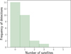 |
Fig. 1. Distribution of the number of satellites detected as [CII] emitters from V20 during an ALMA survey of 27 z ≳ 6 quasars. All these sources reside within ±1000 km s−1, i.e., about ±1.3 Mpc at z = 6.5 from the central quasar. |
ALMA observations of z ∼ 6.5 quasars are characterised by a circular FoV with a radius of ≃90 kpc and cover a wavelength range of Δv = 1000 − 2000 km s−1 with respect to the systematic redshift of each quasar (V20). The explored cosmological volume is thus a cylinder with a base of about 2.6 × 10⁴ kpc2 and a height of about 2.5–5.0 Mpc at z = 6.5, depending on the spectral setting of the observations, as shown in Fig. 2. Here, we focus on the fixed LoS range Δv = 1000 km s−1 to be more conservative because of the large distances involved, and we compare our results with the equivalent sample of V20. Additionally, we consider the median redshift z = 6.5 as representative of the range 6 ≤ z ≤ 7 for the whole sample of V201.
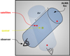 |
Fig. 2. Schematic representation of an ALMA observation of a quasar (yellow star). Here, two galaxy satellites (red stars) are detected, whereas a third satellite remains outside the observer’s cylinder and would be detected only through a different LoS. |
Based on the geometry of the probed volume, the detection rate of companions would depend on both the distribution of galaxies in the quasar environment and on the orientation of the cylinder axis. Therefore, a fair comparison between theoretical studies and observations must take this effect into account.
We created different mock distributions of quasar satellites and studied the frequency of detection when the companions lay within a random observational cylinder. Ideally, we would run numerous, cosmologically motivated, N-body simulations of high-z quasar companions and select a single observational cylinder in each simulation. This approach would be prohibitive in terms of time and computational costs. Alternatively, we ran various sets of Monte Carlo simulations for which we spawned for each set an increasing number of satellites N in the quasar-centred sphere with radius Dz = 6.5, where Dz = 6.5 is the distance corresponding to the recession velocity Δv = 1000 km s−1 at z = 6.5, that is, about 1.3 Mpc. The N satellites represent massive galaxies that are bright enough to be detected by ALMA as [CII] emitters if they fall within the volume probed by the telescope. They indeed represent only the detectable fraction of the whole satellite population, and might in principle be connected to the total dark matter density in which the quasar resides. For each set of simulations (at fixed N), we intersected the quasar-centred sphere with the ALMA cylinder with a random orientation, as exemplified in Fig. 2. In particular, for each given N, we performed 105 simulations for which we varied the position of the satellites, along with the orientation of the observational cylinder. Hence, we computed the probability P(No|N) that No satellites are included in the cylinder, and thus detectable by ALMA, as a function of N. We adopted nine different dark matter distributions to generate the satellite populations, as described below.
– Homogeneous distribution. Satellites were generated by following a homogeneous distribution within the spherical volume, with a fixed radius Dz = 6.5. At z = 6.5, the volume measures about 9 Mpc3. This model is called Homogeneous and represents the simplest case, with no assumptions on the radial distribution.
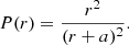
– Plummer model: Satellite galaxies were spawned by following a Plummer density profile (Plummer 1911), with a cumulative distribution function (CDF),
 (1)
(1)
where r is the radius from the central quasar, and a is the scale radius. We adopted two instances for this distribution by choosing a = 25 and 100 kpc. These models are called Plummer25 and Plummer100.
– Hernquist model. Analogously to the Plummer model case, here satellites were generated by mimicking a Hernquist density profile (Hernquist 1990) through the CDF
 (2)
(2)
This model, for which we fixed the scale radius a = 5 kpc, is called Hernquist5.
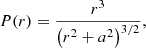
– NFW model. We sampled two Navarro–Frenk–White density profiles (Navarro et al. 1996), called NFW25 and NFW100, via the CDF
![Mathematical equation: $$ \begin{aligned}&P(r) = \mathcal{N} (a) \left[\ln \left(\frac{a+r}{a}\right)-\frac{r}{a+r}\right] \nonumber \\&\mathcal{N} (a) = \left[\ln \left(\frac{a+r_{\rm cut}}{a}\right)-\frac{r_{\rm cut}}{a+r_{\rm cut}}\right]^{-1}, \end{aligned} $$](/articles/aa/full_html/2023/11/aa47172-23/aa47172-23-eq3.gif) (3)
(3)
with scale radii a equal to 25 kpc and 100 kpc, respectively. 𝒩(a) is a normalization constant with rcut = Dz = 6.5.
– CC function. Companion galaxies were randomly spawned by following the cross-correlation function quasar galaxies  , with a = 4.1 comoving Mpc and γ = 1.8 from García-Vergara et al. (2019). In particular, we adopted the CDF
![Mathematical equation: $$ \begin{aligned}&P(r)=\mathcal{N} r^3 \left[\frac{1}{3} + \frac{1}{3-\gamma }\left(\frac{a}{r}\right)^{\gamma }\right] \nonumber \\&\mathcal{N} = r_{\rm cut}^3 \left[\frac{1}{3} + \frac{1}{3-\gamma }\left(\frac{a}{r_{\rm cut}}\right)^{\gamma }\right]^{-1}\!, \end{aligned} $$](/articles/aa/full_html/2023/11/aa47172-23/aa47172-23-eq5.gif) (4)
(4)
where 𝒩 is a normalization constant. This model, called CCF, is only intended to mimic the shape of the galaxy distribution function around quasars. The density was not fixed and varied with N in the Monte Carlo simulations.
– Cosmological simulations. Finally, satellite galaxies were spawned by following the dark matter distribution of cosmological zoom-in simulations of high-redshift quasars. We employed two different cosmological simulations, called CosmoSim1 (Barai et al. 2018) and CosmoSim2 (Valentini et al. 2021). In particular, satellite locations were selected randomly amongst the dark matter potential wells in a z = 6.5 snapshot of each simulation after running the AMIGA halo-finder code (Knollmann & Knebe 2009) with a minimum of 20 bound particles to define a halo. The dark matter haloes were only considered if their distance from the centre of the main halo was Dz = 6.5 at most. CosmoSim1 and CosmoSim2 represent our fiducial models because they were derived from a complex framework that was especially designed to describe the environment of high-z quasars2.
– Although both CosmoSim1 and CosmoSim2 describe the evolution of two very massive dark matter haloes, their virial masses and radii are quite diverse, being Mvir = 3.3 × 10¹² M⊙ and Rvir = 66 kpc, and Mvir = 1.2 × 10¹² M⊙ and Rvir = 47 kpc at z = 6 for CosmoSim1 and CosmoSim2, respectively3 and this increases the generality of the investigation.
– We also note that the feedback prescriptions for the active galactic nuclei are significantly different in the two simulations, and this has a non-negligible impact on the dark-matter distribution (see the effect on the merger history in Zana et al. 2022).
– The models based on the Plummer, Hernquist, and NFW profiles adopt a set of parameters (a and 𝒩) to force their CDFs to have P(r)≳0.99 for r = Dz = 6.5. In the rare occasion when a galaxy was spawned at r > Dz = 6.5, the extraction process was repeated. Because of this expedient measure, the number density of companion galaxies within the spherical volume of radius Dz = 6.5 is directly comparable amongst all the models.
We do not claim that these models completely cover all the possible satellite distributions. They rather aim to probe the implications of highly diverse environments.
3. Results
Figure 3 shows the outcome of the Monte Carlo simulations for the nine satellite distributions. In most cases, the number of detected companions is significantly smaller than N. For example, in the fiducial distribution model CosmoSim1, with three seeded satellites, we estimate P(No = 0|N = 3)=0.29. This indicates that the probability of no detection due to the ALMA FoV is ∼30%, despite the presence of three satellites in the nearby environment. We also observe that satellite distributions based on simulations CosmoSim1 and CosmoSim2 produce almost identical results, although they refer to two distinct quasar hosts. This indicates that a major bias is produced by the observational volume of the telescope that might explain why observations of quasar satellites return so different numbers for detections of serendipitous [CII] emitter.
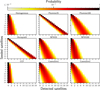 |
Fig. 3. Monte Carlo simulations for all the matter distribution models we adopted, i.e., Homogeneous, Plummer25, Plummer100, Hernquist5, NFW25, NFW100, CCF, CosmoSim1, and CosmoSim2. Each panel shows the probability P(No|N) that No satellites are detected when N satellites are spawned. |
The trace produced by the spherical geometry of NFW25 is very similar to that of the simulation-oriented distributions and might therefore describe a similar distribution of galaxies on average. On the other hand, the distributions in which satellites are almost always spawned in close proximity to the quasar (i.e., Plummer25 or Hernquist5) result in a nearly one-to-one correspondence between seeded and detected satellites. Interestingly, when we distribute a variable number of companion galaxies by following an empirical cross-correlation function quasar-LAEs (CCF), galaxies are generated farther from the quasar, and the detection efficiency drops at higher N. Finally, the outcomes of Homogeneous and NFW100 are similar, even though they are based on very different distribution laws in principle. It is worth mentioning that Homogeneous represents a control scenario that contains no additional conjecture on the galaxy distribution.
The left panel of Fig. 4 shows P(No = N) for all the probed satellite populations. As the seeded population grows, it becomes increasingly challenging to detect all the quasar satellites. P(No = N) is always lower than 1 for N > 0, and it decreases more rapidly the less compact the distribution is. In Sect. 4 we discuss the possibility of sampling a cylinder with a three times larger radius using ALMA. The right panel of Fig. 4 presents the result for this case. It indicates a much higher detection rate.
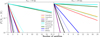 |
Fig. 4. Probability of total detection, P(No = N), for all the density profiles. Left: standard case of Fig. 3, where RFoV ≃ 90 kpc. Right: mosaic case with RFoV ≃ 270 kpc. |
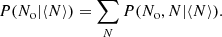
A general quasar environment is better quantified with a mean companion number than with their precise count given the natural variance of a realistic system. Therefore, we introduced a further step to consider the scatter in the number of satellites that can be seeded. In particular, we connected the number N of seeded satellites to the average number ⟨N⟩ of a Poissonian distribution4,
 (5)
(5)
Hence, we can build the conditional probability
 (6)
(6)
and the likelihood function for the average seeded number ⟨N⟩, given a single observation No, P(No|⟨N⟩),
 (7)
(7)
Finally, we computed the distribution 𝒫(⟨N⟩) by including all the detections from V20 and considering them to be equiprobable. Operatively, we multiplied the likelihood associated with every detection and assumed a flat prior over ⟨N⟩,
![Mathematical equation: $$ \begin{aligned} \mathcal{P} (\langle N \rangle )=\frac{\prod _{N_{\rm o}} P(N_{\rm o}|\langle N \rangle )^{f(N_{\rm o})}}{\sum _{N_{\rm o}}\left[\prod _{N_{\rm o}} P(N_{\rm o}|\langle N \rangle )^{f(N_{\rm o})}\right]}, \end{aligned} $$](/articles/aa/full_html/2023/11/aa47172-23/aa47172-23-eq9.gif) (8)
(8)
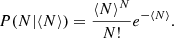
where f(No) is the frequency of detection reported in Fig. 1. The final likelihood functions, reproduced in Fig. 5 for all the distribution models, show that each model has a characteristic peak. As mentioned before, the CCF model predicts the highest number of average intrinsic satellites in order to justify current observations. On the other hand, compact distributions can describe observations with the smallest possible number of satellites. In the specific cases of Plummer20 and Hernquist20, which both sharply peak around ⟨N⟩=1, the observations of V20 with No = 2 or 3 would be explained entirely through Poissonian fluctuations.
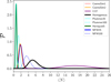 |
Fig. 5. Posterior functions for the different galaxy distributions. The curves show the probability that an average number of massive satellites ⟨N⟩ orbits a z ≳ 6 quasar based on the observed data from V20. The colour-coding is the same as in Fig. 4. |
4. Discussion
Currently, we lack enough observational data to constrain the spatial distribution of galactic companions around high-redshift quasars. For this reason, we have explored various possibilities, each with different degrees of realism and assumptions. While numerical simulations describe the most realistic scenarios, the other radial profiles also offer a reasonable representation of reality, especially due to the limited number of objects involved. Except for the CCF model, which nevertheless has its roots in dedicated observational campaigns, all the spherically symmetric distributions adopted in this work are the radial laws that are most commonly used in astrophysics to model a gravitationally bound system, even if they are not directly connected to the scales and masses studied here. Homogeneous has the fewest assumptions, where galaxies are randomly seeded in the surrounding volume. The other spherically symmetrical models tend to refine the guess and preferentially distribute the galaxies closer to the central quasar. Plummer25, Plummer100, Hernquist5, NFW25, and NFW25 use different radial laws, with different scale radii. Most of the compact distributions, such as Plummer25, Plummer100, and Hernquist5, are less observationally motivated, especially at high N, where numerous companions are spawned within the virial radius of the quasar host, whereas the vast majority of V20 satellites are detected at r > 100 kpc. On the other hand, the relation described by the spherical model CCF is observed to hold for scales larger than Dz = 6.5, beyond the limit of 1000 km s−1.
More consistent models, such as CosmoSim1, CosmoSim2, NFW25, and NFW100, predict ⟨N⟩≳2 on the basis of current observations. This finding has numerous fundamental implications: The geometrical bias of ALMA can explain the scatter in recent observations5. In other words, we support the scenario in which high-z quasars have two massive companions on average, with [CII] luminosities L[CII] ≳ 108 L⊙, but their detection depends on the volume probed by the telescope and thus on the specific LoS of the observation.
This result suggests that for quasar fields in which no satellite has been observed, mosaic observations with ALMA would result in the detection of two new galactic companions per quasar field on average (in the cases described by our fiducial models, ⟨N⟩≃2). In the right panel of Fig. 4, we report the probability P(No = N) as a function of the number of seeded satellites if the FoV is expanded to RFoV ≃ 270 kpc, mimicking an observation with an additional layer of nine adjacent standard FoVs around the original one. For CosmoSim1 and CosmoSim2, in particular, the probability of detecting the whole population of two seeded satellites is 0.72, which is almost six times higher than the probability estimated for a single ALMA pointing (RFoV ≃ 90 kpc). If the intrinsic number of satellites N were instead larger, P(No = N)≳0.5, up to N ∼ 6. Accordingly, follow-up priority should be given to quasar fields that so far have shown the lowest number of companions, based on the high probability of detecting the whole missing population with an individual mosaic observation.
A further consideration can be drawn when we examine our fiducial model, which predicts ⟨N⟩≃2, which agrees very well with the twin model CosmoSim2. Zana et al. (2022) found that a total of two to three satellites were detectable because their [CII] luminosity was higher than the current sensitivity threshold of about 108 L⊙. These results were based on a post-processing study of a suite of cosmological zoom-in simulations, including the evolution of baryons and numerous state-of-the-art sub-grid prescriptions. In the current investigation, we have generalized the dark matter distribution of satellites of such simulations (with no assumptions on the mass of the halo) and demonstrated that current observations (V20) agree remarkably well with our previous prediction. As a consequence, the dense quasar-host environment studied in Zana et al. (2022), which is now confirmed by observations via our geometrical interpretation, likely describes real quasar systems, and this implies that most powerful high-z quasars would live in the densest regions of the Universe.
Finally, we provide an additional interpretation by comparing our predicted number of satellites in the most realistic cases, with recent number-density measurements in a field galaxy population. In the context of the large program ASPECS, Decarli et al. (2020) and Uzgil et al. (2021) have reported no detection of [CII] emitters with L[CII] > 1.89 × 10⁸ L⊙ in the redshift range z ∼ 6 − 8 within a comoving volume of about 12 500 Mpc3, resulting in an upper limit on the galaxy density of 3.4 × 10⁻⁴ Mpc−3. When we consider our predictions to take place within the quasar-centred sphere with radius Dz = 6.5 (the volume enclosing an ALMA cylinder with every possible orientation), our fiducial models lead to a density ≳0.2 Mpc−3, which is higher by almost a factor 600 than the field environment probed by ASPECS. Because no [CII] emitters have been found in the Hubble Ultra Deep Field via ASPECS, this result still holds true even if we computed our detected companions within a larger sphere, where the density might be lower. We conclude by observing that, the analysis we conducted and its findings extend beyond ALMA because they can be applied to any instrument with a limited FoV, due to the straightforward geometric nature of our study.
5. Summary and conclusions
Through various Monte Carlo simulations, we evaluated the geometrical bias of the ALMA telescope for the detection rate of high-z quasar satellites (see Fig. 3). We convolved the resulting probability with a set of Poissonian distributions in order to estimate the intrinsic number of detectable companions that orbit a given quasar potential well. We remark that each detectable satellite represents a galaxy that is massive enough to be detected as a [CII] emitter if it lies within the telescope geometry (see Fig. 2). We produced different likelihood functions for the average number of orbiting satellites in order to explain the most recent ALMA observations (see Fig. 1). Our results are listed below.
-
The telescope bias can entirely explain the differences amongst the number of detected high-z quasar companions. Hence, every quasar could conceivably reside within almost the same environment, but we would detect only a part of the orbiting galaxies, depending on our line of sight.
-
When we consider the most physically motivated distribution profiles, e.g., CosmoSim1 and CosmoSim2, we can infer an intrinsic number of about two satellites that are massive enough to be detected by ALMA as [CII] emitters with L[CII] ≳ 108 L⊙ and that orbit within ∼1.3 Mpc from the quasar.
-
Interestingly, we expect to discover more satellites in the case of CosmoSim1 and CosmoSim2 through a simple mosaic observing campaign that targets the quasars for which no companion galaxies have been observed so far. We predict that a single additional layer of ALMA FoVs around these objects would be enough to observe the total population of N ∼ 2 satellites with a probability of 0.72, compared to 0.13 in the single-observation case. In general, we expect such a campaign to detect the total population of companions half of the time, up to six satellites, that is, P(No = N|N)≳0.5 for N ≲ 6.
-
Our predicted number of satellites (ii) in the case CosmoSim1 is compatible with the analysis performed in Zana et al. (2022). In other words, ALMA observations are consistent with cosmological hydrodynamical simulations evolving z ∼ 6 quasars in the most massive dark matter haloes with Mvir > 1012 − 1013 M⊙, corresponding to fluctuations of about 3 − 4σ in the density field.
-
We compared our fiducial predictions with a recent survey from the ASPECS program, where no [CII] emitters have been confirmed in the field above L[CII] = 1.89 × 10⁸ L⊙ in the same redshift range as we used. This shows once more the over-dense nature of high-z quasar environments.
Future additional ALMA detections of quasar companions will increase our current sample, allowing us to tune this model further and to constrain our predictions better. A contribution may also come from the AtLAST telescope (Klaassen et al. 2020), which, despite its low angular resolution, can detect high-z satellites at a greater distance than ALMA. Follow-up observations of V20 galaxies and the possible detection of supplementary lines could confirm the status of a companion or update the catalogues of quasar satellites. We note, however, that the Poissonian scatter included in our analysis takes these potentially small variations into account. Moreover, the next deep observational campaigns of quasar environments with the James Webb Space Telescope (Gardner et al. 2023) may also help to shed light on the spatial distribution of satellite galaxies because the FoV is much larger. However, the galactic tracers that are probed will be completely different from those of ALMA and will be subject to dust extinction. For this reason, a new and appropriate set of predictions is required.
The ratios amongst the comoving quantities (the position of the satellites and the ALMA observational range) are conserved in redshift. We nonetheless ran our analysis also at different mean redshifts, but found no significant variation.
We also note that only the cosmological simulations, amongst our models, succeeded to reproduce the complex filamentary structures that are expected to form during the collapse of primordial dark matter fluctuations.
We define the virial mass as  , where ρc is the critical density of the Universe, and R200 is the radius enclosing 200 times ρc.
The use of a Poissonian distribution in this context is a commonly made choice. We note that other scatter laws could be adopted with very similar results.
This is valid even before the addition of the Poissonian scatter.
Acknowledgments
Funded by the European Union (ERC, WINGS, 101040227). Views and opinions expressed are however those of the authors only and do not necessarily reflect those of the European Union or the European Research Council Executive Agency. Neither the European Union nor the granting authority can be held responsible for them. TZ and VA acknowledge support from INAF-PRIN 1.05.01.85.08. The authors greatly thank the anonymous referee for useful comments which improved the quality of this manuscript.
References
- Allevato, V., Finoguenov, A., Cappelluti, N., et al. 2011, ApJ, 736, 99 [NASA ADS] [CrossRef] [Google Scholar]
- Allevato, V., Finoguenov, A., Hasinger, G., et al. 2012, ApJ, 758, 47 [NASA ADS] [CrossRef] [Google Scholar]
- Bañados, E., Venemans, B., Walter, F., et al. 2013, ApJ, 773, 178 [CrossRef] [Google Scholar]
- Balmaverde, B., Gilli, R., Mignoli, M., et al. 2017, A&A, 606, A23 [NASA ADS] [CrossRef] [EDP Sciences] [Google Scholar]
- Barai, P., Gallerani, S., Pallottini, A., et al. 2018, MNRAS, 473, 4003 [NASA ADS] [CrossRef] [Google Scholar]
- Capak, P. L., Riechers, D., Scoville, N. Z., et al. 2011, Nature, 470, 233 [Google Scholar]
- Cappelluti, N., Ajello, M., Burlon, D., et al. 2010, ApJ, 716, L209 [NASA ADS] [CrossRef] [Google Scholar]
- Champagne, J. B., Decarli, R., Casey, C. M., et al. 2018, ApJ, 867, 153 [NASA ADS] [CrossRef] [Google Scholar]
- Costa, T., Sijacki, D., Trenti, M., & Haehnelt, M. G. 2014, MNRAS, 439, 2146 [NASA ADS] [CrossRef] [Google Scholar]
- Dashyan, G., Choi, E., Somerville, R. S., et al. 2019, MNRAS, 487, 5889 [NASA ADS] [CrossRef] [Google Scholar]
- Decarli, R., Walter, F., Venemans, B. P., et al. 2017, Nature, 545, 457 [Google Scholar]
- Decarli, R., Walter, F., Venemans, B. P., et al. 2018, ApJ, 854, 97 [Google Scholar]
- Decarli, R., Aravena, M., Boogaard, L., et al. 2020, ApJ, 902, 110 [Google Scholar]
- Di Matteo, T., Khandai, N., DeGraf, C., et al. 2012, ApJ, 745, L29 [NASA ADS] [CrossRef] [Google Scholar]
- Efstathiou, G. 1992, MNRAS, 256, 43P [Google Scholar]
- Ferrara, A., Zana, T., Gallerani, S., & Sommovigo, L. 2023, MNRAS, 520, 3089 [NASA ADS] [CrossRef] [Google Scholar]
- Ferrarese, L., & Ford, H. 2005, Space Sci. Rev., 116, 523 [Google Scholar]
- Fragile, P. C., Anninos, P., Croft, S., Lacy, M., & Witry, J. W. L. 2017, ApJ, 850, 171 [NASA ADS] [CrossRef] [Google Scholar]
- Francis, P. J., & Bland-Hawthorn, J. 2004, MNRAS, 353, 301 [NASA ADS] [CrossRef] [Google Scholar]
- García-Vergara, C., Hennawi, J. F., Barrientos, L. F., & Arrigoni Battaia, F. 2019, ApJ, 886, 79 [CrossRef] [Google Scholar]
- Gardner, J. P., Mather, J. C., Abbott, R., et al. 2023, PASP, 135, 068001 [NASA ADS] [CrossRef] [Google Scholar]
- Habouzit, M., Volonteri, M., Somerville, R. S., et al. 2019, MNRAS, 489, 1206 [CrossRef] [Google Scholar]
- Hall, K. R., Crichton, D., Marriage, T., Zakamska, N. L., & Mandelbaum, R. 2018, MNRAS, 480, 149 [NASA ADS] [CrossRef] [Google Scholar]
- Hennawi, J. F., Prochaska, J. X., Cantalupo, S., & Arrigoni-Battaia, F. 2015, Science, 348, 779 [Google Scholar]
- Hernquist, L. 1990, ApJ, 356, 359 [Google Scholar]
- Hickox, R. C., Jones, C., Forman, W. R., et al. 2009, ApJ, 696, 891 [Google Scholar]
- Husband, K., Bremer, M. N., Stanway, E. R., et al. 2013, MNRAS, 432, 2869 [NASA ADS] [CrossRef] [Google Scholar]
- Intema, H. T., Venemans, B. P., Kurk, J. D., et al. 2006, A&A, 456, 433 [NASA ADS] [CrossRef] [EDP Sciences] [Google Scholar]
- Kashikawa, N., Kitayama, T., Doi, M., et al. 2007, ApJ, 663, 765 [NASA ADS] [CrossRef] [Google Scholar]
- Kikuta, S., Imanishi, M., Matsuoka, Y., et al. 2017, ApJ, 841, 128 [NASA ADS] [CrossRef] [Google Scholar]
- Kim, S., Stiavelli, M., Trenti, M., et al. 2009, ApJ, 695, 809 [NASA ADS] [CrossRef] [Google Scholar]
- Klaassen, P. D., Mroczkowski, T. K., Cicone, C., et al. 2020, in Ground-based and Airborne Telescopes VIII, eds. H. K. Marshall, J. Spyromilio, & T. Usuda, SPIE Conf. Ser., 11445, 114452F [NASA ADS] [Google Scholar]
- Knollmann, S. R., & Knebe, A. 2009, ApJS, 182, 608 [Google Scholar]
- Maiolino, R., Cox, P., Caselli, P., et al. 2005, A&A, 440, L51 [NASA ADS] [CrossRef] [EDP Sciences] [Google Scholar]
- Martín-Navarro, I., Burchett, J. N., & Mezcua, M. 2019, ApJ, 884, L45 [CrossRef] [Google Scholar]
- Martín-Navarro, I., Pillepich, A., Nelson, D., et al. 2021, Nature, 594, 187 [CrossRef] [Google Scholar]
- Mazzucchelli, C., Bañados, E., Venemans, B. P., et al. 2017, ApJ, 849, 91 [Google Scholar]
- Meyer, R. A., Decarli, R., Walter, F., et al. 2022, ApJ, 927, 141 [NASA ADS] [CrossRef] [Google Scholar]
- Mignoli, M., Gilli, R., Decarli, R., et al. 2020, A&A, 642, L1 [EDP Sciences] [Google Scholar]
- Morselli, L., Mignoli, M., Gilli, R., et al. 2014, A&A, 568, A1 [NASA ADS] [CrossRef] [EDP Sciences] [Google Scholar]
- Navarro, J. F., Frenk, C. S., & White, S. D. M. 1996, ApJ, 462, 563 [Google Scholar]
- Neeleman, M., Bañados, E., Walter, F., et al. 2019, ApJ, 882, 10 [Google Scholar]
- Ni, Y., Di Matteo, T., Gilli, R., et al. 2020, MNRAS, 495, 2135 [NASA ADS] [CrossRef] [Google Scholar]
- Okamoto, T., Gao, L., & Theuns, T. 2008, MNRAS, 390, 920 [Google Scholar]
- Planck Collaboration XIII. 2016, A&A, 594, A13 [NASA ADS] [CrossRef] [EDP Sciences] [Google Scholar]
- Plummer, H. C. 1911, MNRAS, 71, 460 [Google Scholar]
- Ross, N. P., Shen, Y., Strauss, M. A., et al. 2009, ApJ, 697, 1634 [NASA ADS] [CrossRef] [Google Scholar]
- Sijacki, D., Springel, V., & Haehnelt, M. G. 2009, MNRAS, 400, 100 [NASA ADS] [CrossRef] [Google Scholar]
- Simpson, J. M., Swinbank, A. M., Smail, I., et al. 2014, ApJ, 788, 125 [Google Scholar]
- Steidel, C. C., Adelberger, K. L., Shapley, A. E., et al. 2005, ApJ, 626, 44 [NASA ADS] [CrossRef] [Google Scholar]
- Swinbank, J., Baker, J., Barr, J., Hook, I., & Bland-Hawthorn, J. 2012, MNRAS, 422, 2980 [NASA ADS] [CrossRef] [Google Scholar]
- Thoul, A. A., & Weinberg, D. H. 1996, ApJ, 465, 608 [NASA ADS] [CrossRef] [Google Scholar]
- Uchiyama, H., Toshikawa, J., Kashikawa, N., et al. 2018, PASJ, 70, S32 [NASA ADS] [CrossRef] [Google Scholar]
- Uchiyama, H., Akiyama, M., Toshikawa, J., et al. 2020, ApJ, 905, 125 [NASA ADS] [CrossRef] [Google Scholar]
- Uzgil, B. D., Oesch, P. A., Walter, F., et al. 2021, ApJ, 912, 67 [Google Scholar]
- Valentini, M., Gallerani, S., & Ferrara, A. 2021, MNRAS, 507, 1 [NASA ADS] [CrossRef] [Google Scholar]
- Venemans, B. P., Röttgering, H. J. A., Miley, G. K., et al. 2007, A&A, 461, 823 [NASA ADS] [CrossRef] [EDP Sciences] [Google Scholar]
- Venemans, B. P., Neeleman, M., Walter, F., et al. 2019, ApJ, 874, L30 [NASA ADS] [CrossRef] [Google Scholar]
- Venemans, B. P., Walter, F., Neeleman, M., et al. 2020, ApJ, 904, 130 [Google Scholar]
- Walter, F., Riechers, D., Cox, P., et al. 2009, Nature, 457, 699 [NASA ADS] [CrossRef] [Google Scholar]
- Wang, F., Yang, J., Fan, X., et al. 2018, ApJ, 869, L9 [NASA ADS] [CrossRef] [Google Scholar]
- Weinberger, R., Springel, V., Pakmor, R., et al. 2018, MNRAS, 479, 4056 [Google Scholar]
- Willott, C. J., Bergeron, J., & Omont, A. 2017, ApJ, 850, 108 [Google Scholar]
- Zana, T., Gallerani, S., Carniani, S., et al. 2022, MNRAS, 513, 2118 [NASA ADS] [CrossRef] [Google Scholar]
All Figures
|
Fig. 1. Distribution of the number of satellites detected as [CII] emitters from V20 during an ALMA survey of 27 z ≳ 6 quasars. All these sources reside within ±1000 km s−1, i.e., about ±1.3 Mpc at z = 6.5 from the central quasar. |
| In the text | |
|
Fig. 2. Schematic representation of an ALMA observation of a quasar (yellow star). Here, two galaxy satellites (red stars) are detected, whereas a third satellite remains outside the observer’s cylinder and would be detected only through a different LoS. |
| In the text | |
|
Fig. 3. Monte Carlo simulations for all the matter distribution models we adopted, i.e., Homogeneous, Plummer25, Plummer100, Hernquist5, NFW25, NFW100, CCF, CosmoSim1, and CosmoSim2. Each panel shows the probability P(No|N) that No satellites are detected when N satellites are spawned. |
| In the text | |
|
Fig. 4. Probability of total detection, P(No = N), for all the density profiles. Left: standard case of Fig. 3, where RFoV ≃ 90 kpc. Right: mosaic case with RFoV ≃ 270 kpc. |
| In the text | |
|
Fig. 5. Posterior functions for the different galaxy distributions. The curves show the probability that an average number of massive satellites ⟨N⟩ orbits a z ≳ 6 quasar based on the observed data from V20. The colour-coding is the same as in Fig. 4. |
| In the text | |
Current usage metrics show cumulative count of Article Views (full-text article views including HTML views, PDF and ePub downloads, according to the available data) and Abstracts Views on Vision4Press platform.
Data correspond to usage on the plateform after 2015. The current usage metrics is available 48-96 hours after online publication and is updated daily on week days.
Initial download of the metrics may take a while.