| Issue |
A&A
Volume 679, November 2023
|
|
|---|---|---|
| Article Number | A35 | |
| Number of page(s) | 20 | |
| Section | Extragalactic astronomy | |
| DOI | https://doi.org/10.1051/0004-6361/202346396 | |
| Published online | 31 October 2023 | |
Influence of star-forming galaxy selection on the galaxy main sequence
1
National Centre for Nuclear Research, Pasteura 7, 02-093 Warszawa, Poland
e-mail: This email address is being protected from spambots. You need JavaScript enabled to view it.
2
Institute of Astronomy, Faculty of Physics, Astronomy and Informatics, Nicolaus Copernicus University, Grudziądzka 5, 87-100 Torua, Poland
3
Aix Marseille Univ. CNRS, CNES, LAM, 38 rue Joliot-Curie, 13388 Marseille, France
4
INAF – Osservatorio di Astrofisica e Scienza dello Spazio, Via P. Gobetti 93/3, 40129 Bologna, Italy
5
Astronomical Observatory of the Jagiellonian University, ul. Orla 171, 30-244 Kraków, Poland
Received:
13
March
2023
Accepted:
29
August
2023
Abstract
Aims. This work aims to determine how the galaxy main sequence (MS) changes using seven different commonly used methods to select the star-forming galaxies within VIPERS data over 0.5 ≤ z < 1.2. The form and redshift evolution of the MS was then compared between selection methods.
Methods. The star-forming galaxies were selected using widely known methods: a specific star-formation rate (sSFR); Baldwin, Phillips, and Terlevich (BPT) diagram; a 4000 Å spectral break (D4000) cut; and four colour-colour cuts (near-ultra-violet – V verses r − J (NUVrJ), near-ultra-violet – V verses r − K (NUVrK), u − r, and U − V verses V − J (UVJ)). The main sequences were then fitted for each of the seven selection methods using a Markov chain Monte Carlo forward modelling routine, fitting both a linear main sequence and a MS with a high-mass turnover to the star-forming galaxies. This was done in four redshift bins of 0.50 ≤ z < 0.62, 0.62 ≤ z < 0.72, 0.72 ≤ z < 0.85, and 0.85 ≤ z < 1.20.
Results. The slopes of all star-forming samples were found to either remain constant or increase with redshift, and the scatters were approximately constant. There is no clear redshift dependency of the presence of a high-mass turnover for the majority of samples, with the NUVrJ and NUVrK being the only samples with turnovers only at low redshift. No samples have turnovers at all redshifts. Star-forming galaxies selected with sSFR and u − r are the only samples to have no high-mass turnover in all redshift bins. The normalisation of the MS increases with redshift, as expected. The scatter around the MS is lower than the ≈0.3 dex typically seen in MS studies for all seven samples.
Conclusions. The lack (or presence) of a high-mass turnover is at least partially a result of the method used to select star-forming galaxies. However, whether a turnover should be present or not is unclear.
Key words: galaxies: evolution / galaxies: formation / galaxies: star formation / galaxies: statistics
© The Authors 2023
 Open Access article, published by EDP Sciences, under the terms of the Creative Commons Attribution License (https://creativecommons.org/licenses/by/4.0), which permits unrestricted use, distribution, and reproduction in any medium, provided the original work is properly cited.
This article is published in open access under the Subscribe to Open model. This email address is being protected from spambots. You need JavaScript enabled to view it. to support open access publication.
1. Introduction
The galaxy main sequence (MS) is an observed tight correlation between the star-formation rate (SFR) and stellar mass (M⋆) of star-forming galaxies (Brinchmann et al. 2004; Noeske et al. 2007; Elbaz et al. 2007). The scatter of this relation is found to be approximately 0.2–0.3 dex, independent of M⋆, and remarkably consistent across the majority of the history of the Universe (e.g. Whitaker et al. 2012; Speagle et al. 2014; Kurczynski et al. 2016; Tomczak et al. 2016; Pearson et al. 2018). This scatter is believed to be a result of fluctuations of in-falling material onto galaxies and periods of intense star-formation (e.g. Abramson et al. 2014; Tacchella et al. 2016; Mitra et al. 2017). The consistency of the scatter is seen to be a result of star formation being dominated by similar slow processes of gradual M⋆ growth in all galaxies at all cosmic times (Lee et al. 2015).
The slope of the MS, or the low-mass MS where a turnover is seen, is typically found to be in the range of 0.4 to 1.0 (Whitaker et al. 2014; Schreiber et al. 2015; Tomczak et al. 2016; Pearson et al. 2018; Popesso et al. 2023). The slope has been seen to reduce towards higher redshift in a small number of studies (e.g. Randriamampandry et al. 2020), while predominantly being seen to increase with redshift in others (e.g. Speagle et al. 2014; Pearson et al. 2018). Further works argue that the slope of the MS should be unity at all redshifts (Pan et al. 2017; Popesso et al. 2023). Slopes of less than unity are considered to be a result of the relative reduction in size of the cold gas reservoir as M⋆ increases along with star-formation quenching (Pan et al. 2017).
Current literature tends to agree on the evolution of the normalisation of the MS. Numerous studies have shown that the normalisation increases with redshift (e.g. Speagle et al. 2014; Schreiber et al. 2015; Tomczak et al. 2016; Pearson et al. 2018; Popesso et al. 2023). This decrease in SFR as the Universe ages may be a result of the availability of cool gas reducing as the redshift decreases (Tacconi et al. 2010; Dunne et al. 2011; Genzel et al. 2015; Scoville et al. 2016; Kokorev et al. 2021). This, coupled with the SFR per dust mass either being constant or increasing with redshift (Tacconi et al. 2010; Scoville et al. 2016), implies an expected increase in SFR with redshift, and hence an increase in the normalisation of the MS with redshift.
The exact form of the MS is highly contested in literature. A number of studies have found that the MS is a simple linear power law of the form log(SFR)∝log(M⋆) at all M⋆ (e.g. Speagle et al. 2014; Pearson et al. 2018). Meanwhile, other studies have found the MS to have a high-mass turnover, with the MS becoming less steep at higher masses (e.g. Whitaker et al. 2012; Lee et al. 2015; Tomczak et al. 2016; Popesso et al. 2019, 2023). This apparent discrepancy has been attributed to how the star-forming galaxies are selected. Johnston et al. (2015) showed that with a more aggressive cut, that is, one that has stricter criteria for a star-forming galaxy, the MS shows less evidence of a high-mass turnover. Similarly, a less aggressive cut shows strong evidence of a turnover. The turnover has also been seen to be a result of the SFR tracer used, as well as the tracer of the MS itself (mean, mode, or median; Popesso et al. 2019).
The selection of star-forming galaxies can be done in a number of different ways. For example, a simple cut in specific star-formation rate (sSFR; e.g. Salim et al. 2018). Alternatively, as star-forming galaxies are typically bluer in colour, a colour or colour-colour cut can be performed. These cuts, such as u − r (e.g. Johnston et al. 2015) or UVJ (e.g. Whitaker et al. 2011, 2014), split the red galaxies, assumed to be quiescent, from the blue galaxies, which are assumed to be star-forming. These colour or colour-colour cuts are often determined semi-visually, by populating the parameter space and observing a clustering of the red and blue galaxies. A line is then drawn between these two clusters to separate the quiescent galaxies from the star-forming galaxies. There are a number of such cuts using different colours, but all functioning using the same underlying logic. The separation of star-forming and quiescent galaxies can also be performed using spectroscopic observations, such as with the Baldwin et al. (1981, BPT) diagram, which requires emission line measurements, or using the strongest discontinuity in the optical spectrum of a galaxy – the 4000 Å break (D4000, Balogh et al. 1999; Gallazzi et al. 2005).
In this work, we studied the form of the MS in the Visible Multi-Object Spectrograph (VIMOS Le Fèvre et al. 2003) Public Extragalactic Redshift Survey1 (VIPERS, Garilli et al. 2014; Guzzo et al. 2014; Scodeggio et al. 2018) using different methods to select the star-forming galaxies, both photometric and spectroscopic. We compare the resulting MSs to understand how selection influences the shape and apparent evolution of the MS. This may help us to understand why some studies find a high-mass turnover in the MS while others do not.
The paper is structured as follows. Section 2 describes the data used along with the star-forming galaxy selection methods, Sect. 3 explains the methodology used to fit the MS, Sect. 4 presents the results, and Sect. 5 provides a discussion. We summarise and conclude in Sect. 6.
2. Data
2.1. VIPERS
This work is based on data from VIPERS. VIPERS is a completed ESO Large Program, which aimed to investigate the spatial distribution of galaxies over the z ∼ 1 Universe (Guzzo et al. 2014; Scodeggio et al. 2018). VIPERS was performed by the VIMOS at moderate resolution (R = 220) using the LR red grism and providing a wavelength coverage of 5500–9500 Å. The galaxy target sample was selected from optical photometric catalogues of the Canada-France-Hawaii Telescope Legacy Survey Wide (CFHTLS-Wide), and covered ∼23.5 deg2 on the sky. The survey was divided into two areas within the W1 and W4 CFHTLS fields. A simple and robust colour pre-selection,
 (1)
(1)
was applied to efficiently remove galaxies at z < 0.5. Moreover, the criterion of iAB < 22.5 mag was used to select the target sample. Finally, VIPERS provided spectroscopic redshifts, spectra, and a full photometrically selected parent catalogue for 86 082 (+530 secondary objects) galaxies.
VIPERS obtained a large volume of 5 × 10⁷h−3 Mpc3 and an average target sampling rate of > 45%. This combination of sampling and depth is uncommon for intermediate redshift surveys at z > 0.5 and places VIPERS as one of a very small number of counterparts of local spectroscopic surveys such as SDSS. Therefore, VIPERS measurements are perfect for studying the evolution of the MS above the local Universe traced by the SDSS.
A detailed description of the survey design and final results can be found in Guzzo et al. (2014) and Scodeggio et al. (2018), respectively. The data reduction pipeline and redshift quality system are described by Garilli et al. (2014). In this work, we used galaxies with spectroscopic redshift quality flags between 3.0 and 4.5, which have a redshift confidence level greater than 95% (Garilli et al. 2014; Scodeggio et al. 2018). The same selection was made in Figueira et al. (2022) to constrain the sets of the SFR calibrators for star forming galaxies and in Siudek et al. (2017) to discuss the star-formation history of passive red galaxies. Applying these cuts gives us a sample of 29 958 galaxies that we used for further analysis.
2.2. Stellar masses and star-formation rates
The stellar masses and SFRs used in this work were derived through spectral energy distribution (SED) modelling using Code Investigating GALaxy Emission (CIGALE, Noll et al. 2009; Boquien et al. 2019) version 2022.1, fitting to broad-band photometry from the far-ultraviolet to the far-infrared, where available. We used a Bruzual & Charlot (2003) stellar population, Chabrier (2003) initial mass function, Charlot & Fall (2000) dust attenuation, Draine et al. (2014) update to the Draine & Li (2007) dust emission, and Fritz et al. (2006) active galactic nucleus (AGN) emission. For the star-formation history (SFH), we used a non-parametric model that does not assume a specific shape of the SFH (Ciesla et al. 2023). A non-parametric model is used to minimise the degeneracy that there is between M⋆ and SFR in SED fitting with parametric SFH models, which can result in bands being formed in the SFR-M⋆ plane and which may influence our results. The parameters used for fitting can be found in Appendix A.
2.3. Emission lines
We performed the analysis of the observed VIPERS spectra (Pistis et al., in prep.) via the penalised pixel fitting code (pPXF Cappellari & Emsellem 2004; Cappellari 2017, 2023). pPXF performs the fit of stellar templates based on the library MILES (Vazdekis et al. 2010) and the fit of the gas templates with the emission lines present in the observed spectral region separately. The gas component is then fitted with a single Gaussian for each emission line giving the integrated fluxes and their errors as a result. For better estimation of the errors, the errors given by pPXF are multiplied by the  of the fit below the line.
To estimate the equivalent widths (EWs) and their error, we built a spectrum with a continuum normalised by dividing the total fit of the spectrum by the fit of the stellar component from pPXF. The resulting normalised spectrum was analysed with specutils, an astropy package for spectroscopy (Astropy Collaboration 2013, 2018) in a range of ±1.06 full width at half maximum (FWHM), which is equivalent to 5σ of the Gaussian fit (Vietri et al. 2022) around the centroid of the emission line.
The quality of the emission line measurements is given by a quality flag (Garilli et al. 2010; Figueira et al. 2022; Pistis et al. 2022) in the form of xyzt. The x value flags lines for which the centroid of the detected line and the centroid of the laboratory observed line is less than 7 Å, the y value flags lines for which the FWHM is between 7 and 22 Å, and the z value flags lines for which the difference between the peak and the fit of the line is less than 30%. The t flags galaxies where the signal-to-noise ratio (S/N) of the EW is at least 3.5 or the S/N of the flux is at least 8 with the number ‘2’, galaxies where the S/N of the EW is at least 3 or the S/N of the flux is at least 7 with the number ‘1’, or flagged with the number ‘0’ otherwise. In this work, for the BPT sample we required the galaxy to have at least one flag set to zero for all three required lines: Hβ, [O III] λ5007, and [O II] λλ3727.
2.4. Star-forming galaxy selection
In this work, we performed seven selections for star-forming galaxies; photometrically, we performed a cut in sSFR, a near-ultra-violet – V verses r − J (NUVrJ) colour cut, a near-ultra-violet – V verses r − K (NUVrJ) colour cut, a u − r colour cut, and a U − V verses V − J (UVJ) colour cut, and spectroscopically we performed BPT selection and a D4000 cut. For all the selections, we required galaxies to have SFR and M⋆ values as well as the required bands, lines, or rest-frame colours for that selection.
The data are also binned by redshift. To determine the edges of the redshift bins, we split the sSFR sample into four bins containing approximately an equal number of galaxies. This results in bins with edges at z = 0.50, z = 0.62, z = 0.72, z = 0.85, and z = 1.20. The differing requirements, described below, resulted in different sample sizes for the different selection methods. The sample sizes for each selection method in each redshift bin can be found in Sect. 4.
We note, however, that any star-forming galaxy selection made will be imperfect. There can be contamination from quiescent galaxies as well as truly star-forming galaxies that are not classified as such, which will vary between the methods used to identify star-forming galaxies. The star-forming galaxy samples can also include transient/E+A galaxies, which are known to contribute up to 8% of quiescent galaxy samples (Vergani et al. 2010) at 0.48 < z < 1.20, and they likely similarly contaminate star-forming galaxy samples.
2.4.1. sSFR
For the cut in sSFR, we visually inspected the SFR-M⋆ plane, as can be seen in Fig. 1, and define star-forming galaxies as follows:
 (2)
(2)
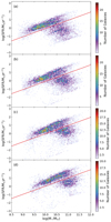 |
Fig. 1. Density plot of SFR versus M⋆ for galaxies with (a) 0.50 ≤ z < 0.62, (b) 0.62 ≤ z < 0.72, (c) 0.72 ≤ z < 0.85, and (d) 0.85 ≤ z < 1.20 from low density (light purple) to high density (dark red). The sSFR cuts are shown as a red lines. |
All 29 958 galaxies in our sample have the required SFR and M⋆, 18 060 of which were selected as star-forming.
2.4.2. NUVrJ
For NUVrJ, we followed Ilbert et al. (2013) to select star-forming galaxies. We thus required star-forming galaxies to have the following:
 (3)
(3)
All 29 958 galaxies in our sample have the required NUV, r, and J observations, 22 868 of which were selected as star-forming. The selection plot can be found in Appendix B. It is possible that the NUVrJ sample can become contaminated with green-valley galaxies as there is no clear delineation between star-forming and green-valley galaxies in the NUVrJ colour-colour space (Ilbert et al. 2010; Moutard et al. 2020).
2.4.3. NUVrK
For NUVrK, we selected the star-forming galaxies as in Davidzon et al. (2016):
 (4)
(4)
All 29 958 galaxies of our sample have the required NUV, r, and K observations, 22 934 of which were selected as star-forming. The selection plot can be found in Appendix B.
While similar to NUVrJ, the r − K colour becomes redder with cosmic time, and it is also sensitive to the inclination of a galaxy. Together with NUV-r, it is therefore a good tracer of the sSFR that is potentially better than NUVrJ at separating active galaxies (Siudek et al. 2018; Moutard et al. 2020). It is also easy for the NUVrK sample to become contaminated with green valley galaxies as there is no clear delineation between star-forming and green-valley galaxies (Moutard et al. 2020).
2.4.4. u − r
We define the selection in u − r after visual examination of the distribution of the rest-frame u − r colour, which we estimated with CIAGLE, as shown in Fig. 2 (Johnston et al. 2015). We select star-forming galaxies as those with u − r < 1.4 at all redshifts. All 29 958 galaxies of our sample have the required rest-frame u − r colour, 18 470 of which were selected as star-forming.
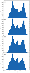 |
Fig. 2. Histogram of rest-frame u − r colour for (a) 0.50 ≤ z < 0.62, (b) 0.62 ≤ z < 0.72, (c) 0.72 ≤ z < 0.85, and (d) 0.85 ≤ z < 1.20. Red lines show the split between star-forming and quiescent galaxies. |
The cut we applied is a bluer cut than that applied by Johnston et al. (2015). As a result, we may be applying a stricter definition of star-forming galaxies and hence be removing more quiescent galaxies. The u − r colour is also sensitive to dust reddening and, as a result, may remove more dusty star-forming galaxies, which typically have a higher M⋆ (e.g. Donevski et al. 2020).
2.4.5. UVJ
For our final star-forming galaxy selection, we used the rest-frame UVJ colour cut of Whitaker et al. (2011) at low redshift:
 (5)
(5)
where the U − V and V − J rest-frame colours were estimated with CIGALE. All 29 958 galaxies of our sample have the required rest-frame U − V and V − J colours, of which 20 371 were selected as star-forming. The selection plot can be found in Appendix B.
The UVJ selection method has been shown to separate quiescent and green-valley galaxies from star-forming galaxies (Moutard et al. 2020). As a result, the UVJ selected star-forming sample should be a relatively pure sample.
2.4.6. BPT
The BPT sample is spectroscopically selected and, as such, contains far fewer galaxies than the photometrically selected samples previously discussed. It should, however, be a much purer star-forming sample than other methods. For BPT-selected star-forming galaxies, we followed the Lamareille (2010) ‘blue BPT’. The blue BPT selects galaxies using Hβ, [O III] λ5007, and [O II] λλ3727 emission lines. We required all emission lines to have a flux signal-to-noise ratio greater than three. We define star-forming galaxies as galaxies with
![Mathematical equation: $$ \begin{aligned} \begin{aligned} \log ([\mathrm {\text{ O}}{\small {\uppercase {\text{ iii}}}} ]/\mathrm{H} \beta )&< \frac{0.11}{\log ([\mathrm {\text{ O}}{\small {\uppercase {\text{ ii}}}} ]/\mathrm{H} \beta ) - 0.92} + 0.85,\\ \log ([\mathrm {\text{ O}}{\small {\uppercase {\text{ iii}}}} ]/\mathrm{H} \beta )&< 0.3. \end{aligned} \end{aligned} $$](/articles/aa/full_html/2023/11/aa46396-23/aa46396-23-eq7.gif) (6)
(6)
Only 6310 galaxies of our sample have the required lines at the required S/N, of which 4560 were selected as star-forming. The selection plot can be found in Appendix B.
2.4.7. D4000
For the final selection, cutting in D4000, we followed Haines et al. (2017) and define star-forming galaxies as
 (7)
(7)
29 955 galaxies of our sample have the required D4000 measurement, 22 010 of which were selected as star-forming. The selection plot can be found in Appendix B.
The limiting value of 1.55 for D4000 was tested based on the sample of VIPERS galaxies by Haines et al. (2017), but the same limit was used for local Universe SDSS galaxies by Kauffmann et al. (2003). The D4000 index is much easier to measure than the selection of emission lines, as it is the manifestation of the strongest discontinuity in the continuum. The wavelength range of VIPERS (5500–9500 Å) makes the calculation of this estimator of whether or not a galaxy is star-forming rather straightforward. Is it the reason why the sample selected based on the D4000 strength is much larger than the one based on the blue BPT diagram. The D4000 selection can also contain a large contamination of more passive galaxies in the star-forming sample, especially at higher M⋆ (Vergani et al. 2008). D4000 is also one of the measurements with the lowest associated error.
2.5. Sample differences
As each star-forming galaxy sample is selected differently, it is informative to see the overlap between the different samples. In Table 1, we present the fraction of the sample selected by the column header that is contained within the sample selected by the header of the row. Due to the requirement that the BPT sample have signal-to-noise ratios greater than three for the four emission lines, Hβ, [O III] λ5007, and [O II] λ3727, this sample contains a small fraction of the other samples, at most 44%. This limitation in sample size is also due to the observations of the required lines being limited to 0.5 < z < 0.9. Hence, the results with the BPT selection should be treated with caution even though it should contain the most obvious sample of star-forming galaxies as all of them are characterised by a very strong set of emission lines. This strict requirement on emission lines reduces the completeness of the sample.
Fraction of star-forming galaxy sample selected with the column header that is present in the star-forming galaxy sample selected with the row header.
It is also important to understand where the samples differ in the SFR-M⋆ plane. We calculated the mean and standard deviations of the SFR in mass bins of 0.25 dex in width (the same M⋆ bins used in the forward modelling described in Sect. 3.1) and present them in Fig. 3. As can be seen, the samples are similar at lower M⋆ (log(M⋆/M⊙ ⪅ 10.5 depending on redshift). At higher mass, sSFR and u − r are more restrictive in selection, while NUVrJ, NUVrK, BPT, and D4000 are less restrictive. The UVJ selection lies between these two extremes.
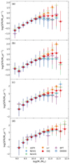 |
Fig. 3. Mean SFR and standard deviation (vertical error bars) of the sSFR (light green stars), NUVrJ (light blue pluses), NVUrK (dark green crosses), u − r (orange, downward pointing triangles), UVJ (red, upward pointing triangles), BPT (empty purple circles), and D4000 (empty dark blue squares) selected star-forming galaxies at (a) 0.50 ≤ z < 0.62, (b) 0.62 ≤ z < 0.72, (c) 0.72 ≤ z < 0.85, and (d) 0.85 ≤ z < 1.20. Horizontal error bars indicate the width of the M⋆ bin. |
3. Methods
3.1. Forward modelling
To fit the MS to our data, we closely followed the Markov chain Monte Carlo method of Pearson et al. (2018). This method fits the parameters of the form of the MS being fitted as well as the scatter of the MS.
For each observed M⋆, a random SFR was drawn from a Gaussian distribution centred on the SFR of the MS being tested at that M⋆. The standard deviation of the Gaussian distribution was the scatter of the MS at that step. The Gaussian distribution was truncated such that it could not produce SFRs larger (smaller) than the largest (smallest) observed SFR. Once the model SFRs had been generated, both the SFR and M⋆ were perturbed by adding a second random number generated from a Gaussian centred on zero and with a standard deviation of 0.25 dex. This was done to simulate the uncertainty in SFR and M⋆.
The model data was then compared to the observed data. The real and simulated data were binned into mass bins of width 0.25 dex. The means and standard deviations of the SFR in these bins were then calculated and the means and standard deviations of the model data were compared to their counterparts from the observed data. The greater the difference, the less likely the model was an accurate representation of the observed data.
In this work, we fitted two forms of the MS to the data: a linear form (Whitaker et al. 2012),
 (8)
(8)
where S is log(SFR/M⊙ yr−1), α is the slope, and β is the normalisation, and a form with a high-mass turnover (Lee et al. 2015),
 (9)
(9)
where S0 is the value of S that the function approaches at high mass, M0 is the turnover mass in M⊙ and γ is the low-mass slope.
3.2. Mass completeness
When determining the mass completeness limit, we followed Pozzetti et al. (2010) and determined this limit empirically. We determined the mass completeness limit for each selection method and in each redshift bin before the star-forming galaxies were selected. For example, for the galaxies with NUV-, r- and J-band magnitudes, we determined the mass limit of the galaxies before we selected the star-forming galaxies that meet the NUVrJ criteria.
Using the Ks-band limiting magnitude of 23.8 (Jarvis et al. 2013), the limit of observable mass for a galaxy (Mlim) can be determined per object with
 (10)
(10)
where M is the galaxy’s mass in M⊙, Ks, lim is the limiting Ks-band magnitude and Ks is the observed Ks-band magnitude. The limiting mass of the sample is then the Mlim below which 90% of the faintest 20% of galaxies have Mlim. The mass completeness limits derived and used in this work are shown in Table 2.
The VIPERS sample’s mass completeness has been determined previously using i-band data in Davidzon et al. (2016) also using the Pozzetti et al. (2010) method. This i-band mass completeness limit was found to be 10.18 < log(M⋆/M⊙) < 10.86 depending on the redshift of the galaxies and if they are star-forming or quiescent. These limits are close to, or just below the mass at which the MS has been seen to turn over (e.g. Lee et al. 2015; Tomczak et al. 2016). Thus, cutting at the i-band limit may hide or remove any evidence of a high-mass turnover in the MS. Moutard et al. (2016) also derived the Ks-band mass completeness limits, again using the Pozzetti et al. (2010) method. However, Moutard et al. (2016) used a Ks magnitude limit of 22, and so found a mass completeness limit approximately 0.5 dex higher than the limit found in this work.
4. Results
The most likely parameters when fitting with Eq. (8) are shown in Fig. 4 and Table 3, while the most likely parameters when fitting with Eq. (9) are shown in Fig. 5 and Table 4. Figure 6 shows the best-fit MSs in the SFR-M⋆ plane for galaxies at 0.50 ≤ z < 0.62. Similar plots for the higher redshift bins can be found in Appendix C.
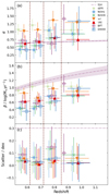 |
Fig. 4. Most likely (a) slope (α), (b) normalisation (β), and (c) scatter of Eq. (8) for sSFR (light green stars), NUVrJ (light blue pluses), NVUrK (dark green crosses), u − r (orange, downward pointing triangles), UVJ (red, upward pointing triangles), BPT (empty purple circles), and D4000 (empty dark blue squares) selected galaxies. Redshifts of markers are offset for clarity. Vertical dashed lines indicate the edges of the redshift bins. Redshifts and their uncertainties are average redshifts of the sample and sample standard deviation. Compilation results of Speagle et al. (2014, S14, lilac dot-dashed line) are included for comparison, using their intrinsic scatter. |
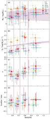 |
Fig. 5. Most likely (a) turn-over mass (M0), (b) SFR that the function approaches at high-mass (S0), (c) low mass slope (γ), and (d) scatter of Eq. (9) for sSFR (light green stars), NUVrJ (light blue pluses), NVUrK (dark green crosses), u − r (orange, downward pointing triangles), UVJ (red, upward pointing triangles), BPT (empty purple circles), and D4000 (empty dark blue squares) selected galaxies. Redshifts of markers are offset for clarity. Vertical dashed lines indicate the edges of the redshift bins. Horizontal dotted lines in (a) indicate the range within which M0 must fall for the MS to be considered to have a turnover. Redshifts and their uncertainties are average redshift of the sample and sample standard deviation. Compilation results of Popesso et al. (2023, P23, lilac dashed line) are included for comparison. Popesso et al. (2023) do not provide a scatter in the MS, so this is omitted from panel d. |
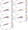 |
Fig. 6. Most likely linear (Eq. (8), blue line) MS and turnover (Eq. (9), red dashed line) MS for star-forming galaxies at 0.5 ≤ z < 0.62 selected with (a) sSFR, (b) NUVrJ, (c) NUVrK, (d) u − r, (e) UVJ, (f) BPT, and (g) D4000. The mean and standard deviation of SFR within a M⋆ bin of width 0.25 dex, used during the forward modelling described in Sect. 3.1, are shown as orange squares and their associated vertical error bar. Horizontal error bar indicates the width of the M⋆ bin. |
To determine if a MS has a turnover, we require the turnover mass to be within the fit-able range of masses of the star-forming galaxies, and the χ2 for the fit with the turnover MS (Eq. (9)) to be lower than the χ2 of the fit with the linear MS (Eq. (8)). Thus, we require M0, the turnover mass, to be in the ranges: 8.8 < log(M0/M⊙) < 11.4 at 0.50 ≤ z < 0.62, 9.0 < log(M0/M⊙) < 11.4 at 0.62 ≤ z < 0.72, 9.2 < log(M0/M⊙) < 11.4 at 0.72 ≤ z < 0.85, and 9.5 < log(M0/M⊙) < 11.2 at 0.85 ≤ z < 1.20. The lower limits were selected by taking the largest lowest mass of any star-forming sample (i.e. after removing the quiescent galaxies) and rounding up to one decimal place, and the upper limits were selected by taking the smallest largest mass of any star-forming sample except D4000, as the D4000 sample is limited to log(M⋆/M⊙) < 11.0 and rounding down to one decimal place.
4.1. sSFR
In fitting Eq. (8) to the sSFR selected galaxies, we find that the slope does not decrease significantly with redshift, with only a slight steepening at 0.62 ≤ z < 0.72, as can be seen in Fig. 4a (light green stars). The normalisation is seen to increase slightly between the first two bins, from 0.92 ± 0.12 to 1.03 ± 0.12, before becoming constant. The scatter remains approximately constant at ≈0.08 dex.
When fitting Eq. (9) to the same sample, we find that M0 rises across the entire redshift range, as shown in Fig. 5a (light green stars). The same trend is seen with S0, with the asymptotic SFR increasing with redshift from z = 0.50 to z = 1.20. The low-mass slope, γ, becomes steeper over 0.50 ≤ z < 0.85 before shallowing in the highest redshift bin, which is different to the trend seen when fitting Eq. (8). The scatter, however, behaves similarly to when fitting Eq. (8), remaining consistent within the error at all redshifts. We find M0 does not fall within the fit-able range at any redshift, and so we find no evidence of a high-mass turnover for the sSFR sample.
4.2. NUVrJ
For the NUVrJ selection, we find that the slope of the linear MS is approximately constant at z < 0.72 before increasing into the 0.72 ≤ z < 0.85 redshift bin and again remaining approximately constant. The normalisation follows a similar trend, as shown in Fig. 4b (light blue pluses). The scatter shows a slight decrease over the entire redshift range studied but remains constant within the error.
For this sample, we find that the M0 of the turnover MS increases with redshift from z = 0.50 to z = 0.85 before dropping out to z = 1.20. The only bin that has M0 outside of the fit-able range is 0.72 ≤ z < 0.85. Of the bins with M0 in the fit-able range, only the lower two redshift bins have a lower χ2 than the linear fits, and hence NUVrJ only shows evidence of a turnover at 0.50 ≤ z < 0.72. S0 follows the same trend as M0, rising over 0.50 ≤ z < 0.85 before falling again. γ generally remains approximately constant across the entire redshift range, with a lower value at 0.62 ≤ z < 0.72. For the scatter, there is a hint that it reduces slightly with redshift but it remains consistent within the error, as can be seen in Fig. 5d (light blue pluses).
4.3. NUVrK
Despite being a very similar selection method to NUVrJ, the NUVrK selection does not follow the NUVrJ trends for the linear MS. The slope is seen to increase across the redshift range, from 0.53 ± 0.25 to 0.92 ± 0.37. The normalisation also increases over the full redshift range. The scatter of the NUVrK selection also differs from the NUVrJ selection in that there is a very slight hint of an increase with redshift, but again it remains consistent within errors, as seen in Fig. 4c (dark green crosses).
For the turnover MS, the trends for NUVrK are similar to those of NUVrJ, as may be expected considering the similarity of the samples. The M0 sees an increase with redshift from z = 0.50 to z = 0.85 before dropping out to z = 1.20. Unlike the NUVrJ sample, however, the M0 of the NUVrK sample remains in the fit-able range at all redshifts. While M0 is in the fit-able range at all redshifts, the highest redshift bin has a lower χ2 for the linear MS, and hence there is only evidence of a high-mass turnover at z < 0.82. The asymptotic SFR of the NUVrK sample also increases across the entire redshift range and does not spike in the 0.72 ≤ z < 0.85 redshift bin, unlike the NUVrJ sample. The low-mass slope values are consistent with the NUVrJ sample, but there is an increasing value of γ over 0.62 ≤ z < 1.20 after falling between the first and second redshift bins. The scatter around the MS again remains consistent in all redshift bins.
4.4. u − r
The linear MS of the u − r-selected star-forming galaxies shows a slight rise in slope with redshift, with a significant rise between 0.62 ≤ z < 0.72 and 0.72 ≤ z < 0.85 and a slight fall into the highest redshift bin, as shown in Fig. 4a (orange, downward pointing triangles). The normalisation remains consistent across all redshift bins, while the scatter around the MS shows a very slight increase over 0.62 ≤ z < 1.20; although, the scatter remains consistent within errors in all redshift bins.
The turnover MS of the u − r-selected star-forming galaxies shows a slight increase in M0 over 0.52 ≤ z < 0.85 before decreasing slightly, but all M0 values are consistent. All but the lowest redshift bin have M0 outside of the fit-able range, but the χ2 in the lowest redshift bin is larger than the linear MS, and, as a result, the u − r selection does not show evidence of a high-mass turnover at any redshift. S0 sees an increase in value out to z = 0.85 before falling slightly into the 0.85 ≤ z < 1.20 redshift bin. The low-mass slope is consistent across all redshift bins but may be slightly lower in the lower two redshift bins when compared to the two higher bins. The scatter of the turnover MS is approximately constant across the entire redshift range.
4.5. UVJ
For the UVJ selection, the slope is seen to increase with redshift along with the normalisation, but both the slope and normalisation are consistent within errors in all redshift bins. As with the other star-forming galaxy selection methods, the scatter for the UVJ selection remains consistent within errors in all redshift bins.
For the turnover MS, M0 shows an increase over 0.52 ≤ z < 0.85 before decreasing slightly. Unlike the u − r selection, the UVJ selection M0 are all within the fit-able region. The χ2 in the 0.62 ≤ z < 0.72 and 0.85 ≤ z < 1.20 redshift bins are also lower than when fitting Eq. (8), and so the UVJ selection shows evidence of a turnover in these two redshift ranges. The trend seen for S0 in Fig. 5a (red, upward pointing triangles) has a general increase across the entire redshift range, but also a notable spike in value at 0.72 ≤ z < 0.85. γ becomes shallower from 0.50 ≤ z < 0.62 to 0.62 ≤ z < 0.72 before becoming steeper out to z = 1.20. Once again, the scatter for the UVJ sample remains consistent in all redshift bins.
4.6. BPT
Due to the requirement of spectral lines in the BPT sample, the average redshift in the highest redshift bin is notably lower than the other samples, a result of the required lines only being observed out to z = 0.9. While fitting Eq. (8), we see the BPT sample has constant slope over 0.50 ≤ z < 0.72 before a very slight, but still consistent, drop in 0.72 ≤ z < 0.85. The highest redshift bin shows a large increase in slope to 1.41 ± 0.47. The normalisation also remains constant out to z = 0.72 but then rises throughout the rest of the redshift range, as seen in Fig. 4b (purple circles). The scatter again remains consistent within error across the entire redshift range.
The MS with a turnover shows a rise in M0 between the lowest and second lowest redshift bins before falling in the higher two redshift bins. All M0 are in the fit-able region while the 0.50 ≤ z < 0.62 and the 0.72 ≤ z < 0.85 redshift bins have lower χ2, indicating that these two bins have evidence of a high-mass turnover. For S0, we see a rising asymptotic SFR with redshift –in Fig. 5b (purple circles)– out to z = 0.85 before it falls into the highest redshift bin. The low-mass slope, γ, decreases between the lowest two redshift bins before rising for the remainder of the redshift range. The BPT sample is the only sample where the scatter does not remain consistent for the turnover MS. The scatter falls between the lowest and second lowest redshift bins as well as between the second highest and the highest. Between the two intermediate redshift bins, the scatter is seen to increase.
4.7. D4000
For the D4000 sample, we find that the slope, α in Eq. (8), increases with redshift from 0.50 ≤ z < 0.62 to 0.85 ≤ z < 1.20. The normalisation also rises with redshift over the full redshift range, as can be seen in Fig. 4b (dark blue stars). Again, we see a scatter than is consistent in all redshift bins.
Fitting with Eq. (9), we find that M0 increase with redshift over 0.50 ≤ z < 1.20 and remains within the fit-able region. As the UVJ sample, the χ2 is smaller for the turnover MS in the 0.62 ≤ z < 0.72 and 0.85 ≤ z < 1.20 redshift bins, so these two redshift ranges show evidence of a high-mass turnover. The value of S0 also increases over the entire redshift range, along with the low-mass slope, as shown in Fig. 5c (dark blue stars). The scatter of the turnover MS remains consistent within error at all redshifts, but there is a slight indication of a rise between z = 0.50 and z = 0.85.
5. Discussion
5.1. Linear main sequence
The slope of the linear MS is generally found to increase with redshift, with the exception of BPT at z < 0.85. This is in line with what is typically found, with many studies finding a slope that increases with redshift (e.g. Speagle et al. 2014; Pearson et al. 2018). While the majority of the samples following similar trends is to be expected, as all samples are drawn from the same survey catalogue, a decreasing slope with redshift for BPT was not expected. A decreasing slope with redshift has previously been seen (Randriamampandry et al. 2020); however, it is not commonly found. The Randriamampandry et al. (2020) MS is derived with radio-selected, star-forming galaxies that have had AGNs removed. Their highest two redshift bins (0.47 ≤ z < 0.83 and 0.83 ≤ z < 1.20) cover a similar range to this work. No reason is given for their decreasing slope. As the BPT sample is significantly smaller than the other samples, this decrease in slope we found for the BPT sample may be a result of this small sample size providing poor constraints on the MS.
A number of the slopes found in this work are above unity, with slopes at or below unity typically found or assumed for the MS (Speagle et al. 2014; Popesso et al. 2023). All slopes for the sSFR and u − r samples are above unity, along with NUVrJ at 0.72 ≤ z < 0.85 and BPT and D4000 at 0.85 ≤ z < 1.20. It is not clear why these specific samples have a slope above unity. The sSFR and u − r samples both show no evidence of a high-mass turnover at all redshifts, so the high slope is not a result of a turnover MS being a better fit, although if this were true we would expect a lower slope, not a higher one. Similarly, NUVrJ at 0.72 ≤ z < 0.85 and BPT at 0.85 ≤ z < 1.20 do not show evidence of a high-mass turnover. D4000 at 0.85 ≤ z < 1.20 does show evidence of a turnover, but again we would expect this to reduce the slope not increase it above unity.
Normalisations of the MSs are more in line with what would typically be expected: rising with redshift (e.g. Speagle et al. 2014; Popesso et al. 2023). The normalisations are typically found to be below those of the Speagle et al. (2014) evolution. The exceptions are the sSFR at z < 0.72 and the BPT at z ≥ 0.85, which have β within the error of the Speagle et al. (2014) trend. As with the slope, none of these three samples have evidence of a high-mass turnover.
The scatters are lower than would typically be expected (e.g. Whitaker et al. 2012; Speagle et al. 2014; Kurczynski et al. 2016; Tomczak et al. 2016; Pearson et al. 2018), with the BPT scatter in the 0.72 ≤ z < 0.85 bin being the largest of all samples at all redshifts at 0.15 ± 0.17. The BPT sample also has the largest scatters of all the star-forming galaxy selections in the lowest and highest redshift bins. This larger scatter for the BPT samples may be a result of the relatively small sample size compared to the other samples. The small overall scatter of the MS for all samples is likely a result of the non-parametric SFH used. Using the same VIPERS galaxies with a parametric SFH from Moutard et al. (2016) produces a linear MS with a much larger scatter, larger than the 0.3 dex typically found.
5.2. Turnover main sequence
Not all the star-forming galaxy samples’ MSs show evidence of a high-mass turnover. All galaxy samples used SFRs derived in the same way, here from SED fitting, and all MS were fitted in the same way (as described in Sect. 3.1). As only the selection criteria differ between samples, this would suggest that the selection method used to identify star-forming galaxies is a key component in the presence, or lack, of a high-mass turn-over. This supports previous works that arrived at the same conclusion (e.g. Renzini & Peng 2015). However, this does not exclude different SFR tracers or different MS tracers resulting in the presence (or absence) of a high-mass turnover, as found by Popesso et al. (2019). Together, these suggest that the form of the MS is an artefact, but it does not highlight which form is correct: if it is the high-mass turnover or the lack of the high-mass turn-over that is an artefact.
The redshifts where the different samples show little evidence of a high-mass turnover are typically at lower redshifts, z < 0.72, although there are a few turnovers found at higher redshifts. NUVrK, UVJ, BPT, and D4000 find one turnover each at z ≥ 0.72, while the other seven samples with high-mass turnovers are all at z < 0.72. Stronger turnovers of the MS are typically found at lower redshifts (Whitaker et al. 2014; Lee et al. 2015; Tomczak et al. 2016; Popesso et al. 2023), thus revealing weaker, or no, turnovers in all but the NUVrJ and NUVrK star-forming samples at lower redshifts was not to be expected. This does, however, agree with what is seen in our highest redshift bin, 0.85 ≤ z < 1.20, which only has turnovers for UVJ and D4000.
Selecting with NUVrJ or NUVrK find turnovers at z < 0.72 and z < 0.85, respectively. As these two samples are similar types of cuts, it is not surprising to find similar results. As the turnover disappears at higher redshifts, these two samples support the commonly found observation that higher redshift samples have a weaker, or no, turnover than their lower redshift counterparts. This would suggest that the higher mass galaxies that are considered to be star-forming by these two selections are less efficient in forming stars in the older Universe than in the younger Universe. These two samples may also be contaminated by green valley galaxies, which may also be helping to create the high-mass turnovers seen.
The sSFR and u − r samples are the only selections that do not contain a redshift bin that shows evidence of a turnover, and sSFR is the only selection that does not have a redshift bin with M0 within the fit-able region. The sSFR selection is very strict in rejecting passive galaxies. With the sSFR cut being so close the MS and the tight scatter, it is not surprising that this sample was found to be linear. Similarly, the u − r sample does not show many low star-formation objects in the sample -with only a low number at higher masses- suggesting that the u − r selection is relatively strict in removing passive galaxies, resulting in a linear MS. The u − r selection may also be removing dusty star-forming galaxies due to its sensitivity to dust attenuation. As dusty galaxies are typically high mass, this may also be contributing to the lack of a high-mass turnover for the u − r sample.
For the UVJ, BPT, and D4000 samples, there is no redshift trend in terms of where they see a turn-over. UVJ and D4000 see turnovers at 0.62 ≤ z < 0.72 and 0.85 ≤ z < 1.20 while BPT sees turn-overs at 0.50 ≤ z < 0.62 and 0.72 ≤ z < 0.85. If a turnover is a result of quiescent contamination of the star-forming sample and the BPT sample is the most conservative in selecting star-forming galaxies, it would be expected that all star-forming samples have turnovers at least at the same redshifts. This is evidently not the case, suggesting that the BPT sample may not necessarily be the purest star-forming sample. As the D4000 samples are known to be contaminated by quiescent galaxies (Vergani et al. 2008) and our D4000 sample turnovers also have no relation to redshift, the BPT sample may contain contaminants. Alternatively, the turnover is not the result of quiescent contamination in the star-forming sample.
5.3. Comparison with other works
Here, we compare our work to literature results gained using the same, or similar, star-forming galaxy selection methods. The NUVrJ selected MSs of Lee et al. (2015), Davidzon et al. (2017), and Leslie et al. (2020) all show high-mass turnovers at all redshifts. Lee et al. (2015) study galaxies with z ≤ 1.3 from the multi-wavelength Cosmic Evolution Survey field (COSMOS Scoville et al. 2007) and derive M⋆ and SFR with SED fitting. Davidzon et al. (2017) use z < 6.0 COSMOS galaxies from the Laigle et al. (2016) catalogue and determine M⋆ and SFR by SED fitting with Le Phare (Arnouts et al. 1999; Ilbert et al. 2006). The last of these three studies, Leslie et al. (2020), also used the Laigle et al. (2016) catalogue combined with VLA-COSMOS 3 GHz Large Project (Smolčić et al. 2017) radio data for galaxies out to z ≈ 5.0 and determined SFR through the radio-infrared correlation (Molnár et al. 2018) and M⋆ through SED fitting. All three studies show an increase in normalisation and low-mass slope with redshift. For the NUVrJ selected galaxies in this work, we do not find any turnovers in our highest two redshift bins (0.72 ≤ z < 1.20). The normalisation that we find, β and S0, does increase with redshift, although our low-mass slope also remains approximately constant with redshift. Thus, this work is in partial agreement with the existing literature, more so at low redshift than high.
For NUVrK, Ilbert et al. (2015) found a turnover at all redshifts (0.2 < z < 1.4), unlike this work, which only found turnovers at lower redshifts (0.50 ≤ z < 0.85). Ilbert et al. (2015) also found an increase in normalisation and low-mass slope. As has been stated already, in this work we found an increase in normalisation with redshift as well as an increase in the low-mass slope with redshift above z = 0.62. Thus, our NUVrK results are in reasonable agreement with the existing literature. The Ilbert et al. (2015) results are based on a 24 μm selected sample with M⋆s estimated by SED fitting with Le Phare, while the SFR is derived from the total infrared emission summed with the total ultra-violet (UV) emission (Arnouts et al. 2013).
With the UVJ selection of NEWFIRM Medium-Band Survey (Whitaker et al. 2011) galaxies, Whitaker et al. (2012) found a weak turnover at 0.50 < z < 1.0 that becomes more apparent as redshift increases, out to z = 2.5. The M⋆s in Whitaker et al. (2012) were estimated via SED fitting with FAST (Kriek et al. 2009), and the SFR was estimated by summing the total infrared and UV emissions (Kennicutt 1998). This turnover evolution is not what is seen in the work, with no turnover present at 0.50 ≤ z < 0.62 or 0.72 ≤ z < 0.85. However, as the redshift bins that we find to have high-mass turnover are in and partially in the 0.5 < z < 1.0 range, it is possible that if we fitted to such a redshift range a turnover would be come apparent. As a turnover is seen in our 0.85 ≤ z < 1.20 redshift range, it is also possible that a turnover would be seen using the Whitaker et al. (2012) 1.0 < z < 1.5 redshift binning.
In a more recent work with UVJ selection, Whitaker et al. (2014) found a weaker turnover as redshift increases and a non-evolving low mass slope. Our UVJ results do not have a clear redshift evolution of the turnover MS. The γ evolution we found also sees the low-mass slope increasing with redshift from z = 0.62. Whitaker et al. (2014) again used FAST to fit SEDs and estimate the M⋆, while the SFR is once again determined by combining the UV and infrared emission (Whitaker et al. 2014) from CANDELS (Grogin et al. 2011), 3D-HST (Brammer et al. 2012), and 24 μm observations over 0.5 < z < 2.5.
The Pearson et al. (2018) UVJ-selected MS shows no high-mass turnover at any redshift (0.2 < z < 6.0). These galaxies are far-infrared-selected with M⋆s and SFRs estimated by SED fitting with CIGALE (Boquien et al. 2019) with a parametric SFH. This lack of turnover agrees with what we see for half of our redshift bins. Pearson et al. (2018) found a slope that increases with redshift, in agreement with our results at z > 0.62. The inclusion of far-infrared data for the SFR estimation in Pearson et al. (2018) may be the cause of this discrepancy. Higher redshift galaxies are more dusty (e.g. Dunne et al. 2011; Donevski et al. 2020), and this may cause an underestimation of the SFR of high-mass galaxies, resulting in a shallower slope at a higher redshift.
5.4. Form of the main sequence
Evidently, different star-forming galaxy selections present different forms of the MS. As a result, the high-mass turnover seen in some studies is likely a result of the method used to select the star-forming galaxies. It is likely that stricter selections result in a more linear MS, while a selection with greater chance of quiescent contamination will result in a MS with a turnover.
6. Summary and conclusions
In this work, we studied the effect of galaxy selection on the MS. We selected star-forming galaxies photometrically using sSFR, NUVrJ, NUVrK, u − r and UVJ, and spectroscopically using BPT and D4000 cuts from the VIPERS sample over 0.5 ≤ z < 1.2. The selected star-forming galaxies were then fitted with both a linear MS and a MS with a high-mass turnover.
The slope of all star-forming samples were found to either remain constant or increase with redshift, the normalisation was also constant or increasing with redshift, while the scatters remained approximately constant. No galaxy samples had turnovers at all redshifts, and only the NUVrJ and NUVrK galaxy samples had a clear redshift evolution of the presence of a high-mass turnover. The sSFR and u − r-selected galaxies show no high-mass turnover at any redshift. There is not a redshift bin for which all the remaining samples showed a high-mass turnover.
As a result, it is apparent that the presence of a high-mass turnover, or lack thereof, is at least partially a result of the galaxy selection method. As we used the same parent sample of galaxies, if this were not the case all different selection methods used would result in either the presence or lack of a high-mass turnover. However, we cannot exclude the possibility that there are other influences on the presence of a high-mass turnover in the MS, such as the tracer used to fit the MS (mean, mode, or median; Popesso et al. 2019) or the SFR tracer used.
Acknowledgments
We would like to thank the referee for their thorough and thoughtful comments that helped improve the quality and clarity of this paper. We would like to thank L. Cielsa for providing the sfrNlevels module for CIGALE. W.J.P. has been supported by the Polish National Science Center project UMO-2020/37/B/ST9/00466 and by the Foundation for Polish Science (FNP). M.F. has been supported by the First TEAM grant of the Foundation for Polish Science No. POIR.04.04.00-00-5D21/18-00 (PI: A. Karska) K.M has been supported by the Polish National Science Center project UMO-2018/30/E/ST9/00082. This work has been partially supported by the Polish National Science Center project UMO-2018/30/M/ST9/00757 and Polish Ministry of Science and Higher Education grant DIR/WK/2018/12. This paper uses data from the VIMOS Public Extragalactic Redshift Survey (VIPERS). VIPERS has been performed using the ESO Very Large Telescope, under the “Large Programme” 182.A-0886. The participating institutions and funding agencies are listed http://vipers.inaf.it.
References
- Abramson, L. E., Kelson, D. D., Dressler, A., et al. 2014, ApJ, 785, L36 [NASA ADS] [CrossRef] [Google Scholar]
- Arnouts, S., Cristiani, S., Moscardini, L., et al. 1999, MNRAS, 310, 540 [Google Scholar]
- Arnouts, S., Le Floc’h, E., Chevallard, J., et al. 2013, A&A, 558, A67 [NASA ADS] [CrossRef] [EDP Sciences] [Google Scholar]
- Astropy Collaboration (Robitaille, T. P., et al.) 2013, A&A, 558, A33 [NASA ADS] [CrossRef] [EDP Sciences] [Google Scholar]
- Astropy Collaboration (Price-Whelan, A. M., et al.) 2018, AJ, 156, 123 [Google Scholar]
- Baldwin, J. A., Phillips, M. M., & Terlevich, R. 1981, PASP, 93, 5 [Google Scholar]
- Balogh, M. L., Morris, S. L., Yee, H. K. C., Carlberg, R. G., & Ellingson, E. 1999, ApJ, 527, 54 [Google Scholar]
- Boquien, M., Burgarella, D., Roehlly, Y., et al. 2019, A&A, 622, A103 [NASA ADS] [CrossRef] [EDP Sciences] [Google Scholar]
- Brammer, G. B., van Dokkum, P. G., Franx, M., et al. 2012, ApJS, 200, 13 [Google Scholar]
- Brinchmann, J., Charlot, S., White, S. D. M., et al. 2004, MNRAS, 351, 1151 [Google Scholar]
- Bruzual, G., & Charlot, S. 2003, MNRAS, 344, 1000 [NASA ADS] [CrossRef] [Google Scholar]
- Calzetti, D., Armus, L., Bohlin, R. C., et al. 2000, ApJ, 533, 682 [NASA ADS] [CrossRef] [Google Scholar]
- Cappellari, M. 2017, MNRAS, 466, 798 [Google Scholar]
- Cappellari, M. 2023, MNRAS, 526, 3273 [NASA ADS] [CrossRef] [Google Scholar]
- Cappellari, M., & Emsellem, E. 2004, PASP, 116, 138 [Google Scholar]
- Chabrier, G. 2003, PASP, 115, 763 [Google Scholar]
- Charlot, S., & Fall, S. M. 2000, ApJ, 539, 718 [Google Scholar]
- Ciesla, L., Gómez-Guijarro, C., Buat, V., et al. 2023, A&A, 672, A191 [NASA ADS] [CrossRef] [EDP Sciences] [Google Scholar]
- Davidzon, I., Cucciati, O., Bolzonella, M., et al. 2016, A&A, 586, A23 [NASA ADS] [CrossRef] [EDP Sciences] [Google Scholar]
- Davidzon, I., Ilbert, O., Laigle, C., et al. 2017, A&A, 605, A70 [NASA ADS] [CrossRef] [EDP Sciences] [Google Scholar]
- Donevski, D., Lapi, A., Małek, K., et al. 2020, A&A, 644, A144 [NASA ADS] [CrossRef] [EDP Sciences] [Google Scholar]
- Draine, B. T., & Li, A. 2007, ApJ, 657, 810 [CrossRef] [Google Scholar]
- Draine, B. T., Aniano, G., Krause, O., et al. 2014, ApJ, 780, 172 [Google Scholar]
- Dunne, L., Gomez, H. L., da Cunha, E., et al. 2011, MNRAS, 417, 1510 [NASA ADS] [CrossRef] [Google Scholar]
- Elbaz, D., Daddi, E., Le Borgne, D., et al. 2007, A&A, 468, 33 [NASA ADS] [CrossRef] [EDP Sciences] [Google Scholar]
- Figueira, M., Pollo, A., Małek, K., et al. 2022, A&A, 667, A29 [NASA ADS] [CrossRef] [EDP Sciences] [Google Scholar]
- Fritz, J., Franceschini, A., & Hatziminaoglou, E. 2006, MNRAS, 366, 767 [Google Scholar]
- Gallazzi, A., Charlot, S., Brinchmann, J., White, S. D. M., & Tremonti, C. A. 2005, MNRAS, 362, 41 [Google Scholar]
- Garilli, B., Fumana, M., Franzetti, P., et al. 2010, PASP, 122, 827 [Google Scholar]
- Garilli, B., Guzzo, L., Scodeggio, M., et al. 2014, A&A, 562, A23 [NASA ADS] [CrossRef] [EDP Sciences] [Google Scholar]
- Genzel, R., Tacconi, L. J., Lutz, D., et al. 2015, ApJ, 800, 20 [Google Scholar]
- Grogin, N. A., Kocevski, D. D., Faber, S. M., et al. 2011, ApJS, 197, 35 [NASA ADS] [CrossRef] [Google Scholar]
- Guzzo, L., Scodeggio, M., Garilli, B., et al. 2014, A&A, 566, A108 [NASA ADS] [CrossRef] [EDP Sciences] [Google Scholar]
- Haines, C. P., Iovino, A., Krywult, J., et al. 2017, A&A, 605, A4 [NASA ADS] [CrossRef] [EDP Sciences] [Google Scholar]
- Ilbert, O., Arnouts, S., McCracken, H. J., et al. 2006, A&A, 457, 841 [NASA ADS] [CrossRef] [EDP Sciences] [Google Scholar]
- Ilbert, O., Salvato, M., Le Floc’h, E., et al. 2010, ApJ, 709, 644 [Google Scholar]
- Ilbert, O., McCracken, H. J., Le Fèvre, O., et al. 2013, A&A, 556, A55 [NASA ADS] [CrossRef] [EDP Sciences] [Google Scholar]
- Ilbert, O., Arnouts, S., Le Floc’h, E., et al. 2015, A&A, 579, A2 [NASA ADS] [CrossRef] [EDP Sciences] [Google Scholar]
- Jarvis, M. J., Bonfield, D. G., Bruce, V. A., et al. 2013, MNRAS, 428, 1281 [Google Scholar]
- Johnston, R., Vaccari, M., Jarvis, M., et al. 2015, MNRAS, 453, 2540 [Google Scholar]
- Kauffmann, G., Heckman, T. M., White, S. D. M., et al. 2003, MNRAS, 341, 33 [Google Scholar]
- Kennicutt, R. C., Jr 1998, ARA&A, 36, 189 [NASA ADS] [CrossRef] [Google Scholar]
- Kokorev, V. I., Magdis, G. E., Davidzon, I., et al. 2021, ApJ, 921, 40 [NASA ADS] [CrossRef] [Google Scholar]
- Kriek, M., van Dokkum, P. G., Labbé, I., et al. 2009, ApJ, 700, 221 [Google Scholar]
- Kurczynski, P., Gawiser, E., Acquaviva, V., et al. 2016, ApJ, 820, L1 [NASA ADS] [CrossRef] [Google Scholar]
- Laigle, C., McCracken, H. J., Ilbert, O., et al. 2016, ApJS, 224, 24 [Google Scholar]
- Lamareille, F. 2010, A&A, 509, A53 [CrossRef] [EDP Sciences] [Google Scholar]
- Lee, N., Sanders, D. B., Casey, C. M., et al. 2015, ApJ, 801, 80 [Google Scholar]
- Le Fèvre, O., Saisse, M., & Mancini, D. 2003, SPIE Conf. Ser., 4841, 1670 [Google Scholar]
- Leslie, S. K., Schinnerer, E., Liu, D., et al. 2020, ApJ, 899, 58 [Google Scholar]
- Mitra, S., Davé, R., Simha, V., & Finlator, K. 2017, MNRAS, 464, 2766 [NASA ADS] [CrossRef] [Google Scholar]
- Molnár, D. C., Sargent, M. T., Delhaize, J., et al. 2018, MNRAS, 475, 827 [Google Scholar]
- Moutard, T., Arnouts, S., Ilbert, O., et al. 2016, A&A, 590, A103 [NASA ADS] [CrossRef] [EDP Sciences] [Google Scholar]
- Moutard, T., Malavasi, N., Sawicki, M., Arnouts, S., & Tripathi, S. 2020, MNRAS, 495, 4237 [CrossRef] [Google Scholar]
- Noeske, K. G., Weiner, B. J., Faber, S. M., et al. 2007, ApJ, 660, L43 [CrossRef] [Google Scholar]
- Noll, S., Burgarella, D., Giovannoli, E., et al. 2009, A&A, 507, 1793 [NASA ADS] [CrossRef] [EDP Sciences] [Google Scholar]
- Pan, Z., Zheng, X., & Kong, X. 2017, ApJ, 834, 39 [Google Scholar]
- Pearson, W. J., Wang, L., Hurley, P. D., et al. 2018, A&A, 615, A146 [NASA ADS] [CrossRef] [EDP Sciences] [Google Scholar]
- Pistis, F., Pollo, A., Scodeggio, M., et al. 2022, A&A, 663, A162 [NASA ADS] [CrossRef] [EDP Sciences] [Google Scholar]
- Popesso, P., Concas, A., Morselli, L., et al. 2019, MNRAS, 483, 3213 [Google Scholar]
- Popesso, P., Concas, A., Cresci, G., et al. 2023, MNRAS, 519, 1526 [Google Scholar]
- Pozzetti, L., Bolzonella, M., Zucca, E., et al. 2010, A&A, 523, A13 [NASA ADS] [CrossRef] [EDP Sciences] [Google Scholar]
- Randriamampandry, S. M., Vaccari, M., & Hess, K. M. 2020, MNRAS, 499, 948 [NASA ADS] [CrossRef] [Google Scholar]
- Renzini, A., & Peng, Y.-J. 2015, ApJ, 801, L29 [Google Scholar]
- Salim, S., Boquien, M., & Lee, J. C. 2018, ApJ, 859, 11 [Google Scholar]
- Schreiber, C., Pannella, M., Elbaz, D., et al. 2015, A&A, 575, A74 [NASA ADS] [CrossRef] [EDP Sciences] [Google Scholar]
- Scodeggio, M., Guzzo, L., Garilli, B., et al. 2018, A&A, 609, A84 [NASA ADS] [CrossRef] [EDP Sciences] [Google Scholar]
- Scoville, N., Aussel, H., Brusa, M., et al. 2007, ApJS, 172, 1 [Google Scholar]
- Scoville, N., Sheth, K., Aussel, H., et al. 2016, ApJ, 820, 83 [Google Scholar]
- Siudek, M., Małek, K., Scodeggio, M., et al. 2017, A&A, 597, A107 [NASA ADS] [CrossRef] [EDP Sciences] [Google Scholar]
- Siudek, M., Małek, K., Pollo, A., et al. 2018, A&A, 617, A70 [NASA ADS] [CrossRef] [EDP Sciences] [Google Scholar]
- Smolčić, V., Delvecchio, I., Zamorani, G., et al. 2017, A&A, 602, A2 [NASA ADS] [CrossRef] [EDP Sciences] [Google Scholar]
- Speagle, J. S., Steinhardt, C. L., Capak, P. L., & Silverman, J. D. 2014, ApJS, 214, 15 [Google Scholar]
- Tacchella, S., Dekel, A., Carollo, C. M., et al. 2016, MNRAS, 457, 2790 [Google Scholar]
- Tacconi, L. J., Genzel, R., Neri, R., et al. 2010, Nature, 463, 781 [Google Scholar]
- Tomczak, A. R., Quadri, R. F., Tran, K.-V. H., et al. 2016, ApJ, 817, 118 [Google Scholar]
- Vazdekis, A., Sánchez-Blázquez, P., Falcón-Barroso, J., et al. 2010, MNRAS, 404, 1639 [NASA ADS] [Google Scholar]
- Vergani, D., Scodeggio, M., Pozzetti, L., et al. 2008, A&A, 487, 89 [NASA ADS] [CrossRef] [EDP Sciences] [Google Scholar]
- Vergani, D., Zamorani, G., Lilly, S., et al. 2010, A&A, 509, A42 [NASA ADS] [CrossRef] [EDP Sciences] [Google Scholar]
- Vietri, G., Garilli, B., Polletta, M., et al. 2022, A&A, 659, A129 [NASA ADS] [CrossRef] [EDP Sciences] [Google Scholar]
- Whitaker, K. E., Labbé, I., van Dokkum, P. G., et al. 2011, ApJ, 735, 86 [Google Scholar]
- Whitaker, K. E., van Dokkum, P. G., Brammer, G., & Franx, M. 2012, ApJ, 754, L29 [Google Scholar]
- Whitaker, K. E., Franx, M., Leja, J., et al. 2014, ApJ, 795, 104 [NASA ADS] [CrossRef] [Google Scholar]
Appendix A: CIGALE model
For the CIGALE models, we used a non-parametric SFH (Ciesla et al. 2023, sfhNlevels), Bruzual & Charlot (2003, bc03) stellar population, Chabrier (2003) initial mass function, Charlot & Fall (2000, dustatt_2powerlaws) dust attenuation, Draine et al. (2014, dl2014) dust emission, and Fritz et al. (2006, fritz2006) AGN emission. The parameters used in CIGALE can be found in Table A.1.
Parameters used for the CIGALE model SEDs used to estimate M⋆ and SFR, and the u-r, U-V, and V-J rest-frame colours.
Appendix B: Star-forming galaxy selection plots
Here, we present the star-forming-galaxy selection plots for the NUVrJ selection in Fig. B.1, the NUVrK selection in Fig. B.2, the UVJ selection in Fig. B.3, the BPT selection in Fig. B.4, and the D4000 selection in Fig. B.5.
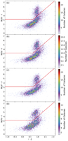 |
Fig. B.1. Density plot of NUV-r versus r-J for galaxies with (a) 0.50 ≤ z < 0.62, (b) 0.62 ≤ z < 0.72, (c) 0.72 ≤ z < 0.85, and (d) 0.85 ≤ z < 1.20 from low density (light purple) to high density (dark red). The NUVrJ cuts are shown as a red lines. |
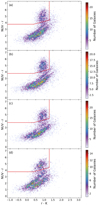 |
Fig. B.2. Density plot of NUV-r versus r-K for galaxies with (a) 0.50 ≤ z < 0.62, (b) 0.62 ≤ z < 0.72, (c) 0.72 ≤ z < 0.85, and (d) 0.85 ≤ z < 1.20 from low density (light purple) to high density (dark red). The NUVrK cuts are shown as a red lines. |
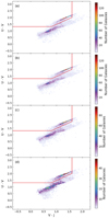 |
Fig. B.3. Density plot of U-V versus V-J for galaxies with (a) 0.50 ≤ z < 0.62, (b) 0.62 ≤ z < 0.72, (c) 0.72 ≤ z < 0.85, and (d) 0.85 ≤ z < 1.20 from low density (light purple) to high density (dark red). The UVJ cuts are shown as a red lines. |
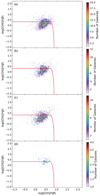 |
Fig. B.4. Density plot of log([O III]/Hβ) versus log([O II]/Hβ for galaxies with (a) 0.50 ≤ z < 0.62, (b) 0.62 ≤ z < 0.72, (c) 0.72 ≤ z < 0.85, and (d) 0.85 ≤ z < 1.20 from low density (light purple) to high density (dark red). The BPT cuts are shown as a red lines. |
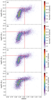 |
Fig. B.5. Density plot of M⋆ versus D4000 for galaxies with (a) 0.50 ≤ z < 0.62, (b) 0.62 ≤ z < 0.72, (c) 0.72 ≤ z < 0.85, and (d) 0.85 ≤ z < 1.20 from low density (light purple) to high density (dark red). The D4000 cuts are shown as a red lines. |
Appendix C: Further main sequence plots
Here, we present the best-fit linear and turnover MSs in the SFR-M⋆ plane for galaxies at 0.62 ≤ z < 0.72 (Fig. C.1), 0.72 ≤ z < 0.85 (Fig. C.2), and 0.85 ≤ z < 1.20 (Fig. C.3). A similar plot for galaxies at 0.50 ≤ z < 0.62 can be found in Fig. 6.
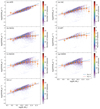 |
Fig. C.1. Most likely linear (Eq. 8, blue line) MS and turnover (Eq. 9, red dashed line) MS for star-forming galaxies at 0.62 ≤ z < 0.72 selected with (a) sSFR, (b) NUVrJ, (c) NUVrK, (d) u-r, (e) UVJ, (f) BPT, and (g) D4000. The mean and standard deviations of SFR within a M⋆ bin of 0.25 dex in width, used during the forward modelling described in Sect. 3.1, are shown as orange squares, and we show their associated vertical error bar. The horizontal error bar indicates the width of the M⋆ bin. |
All Tables
Fraction of star-forming galaxy sample selected with the column header that is present in the star-forming galaxy sample selected with the row header.
Parameters used for the CIGALE model SEDs used to estimate M⋆ and SFR, and the u-r, U-V, and V-J rest-frame colours.
All Figures
|
Fig. 1. Density plot of SFR versus M⋆ for galaxies with (a) 0.50 ≤ z < 0.62, (b) 0.62 ≤ z < 0.72, (c) 0.72 ≤ z < 0.85, and (d) 0.85 ≤ z < 1.20 from low density (light purple) to high density (dark red). The sSFR cuts are shown as a red lines. |
| In the text | |
|
Fig. 2. Histogram of rest-frame u − r colour for (a) 0.50 ≤ z < 0.62, (b) 0.62 ≤ z < 0.72, (c) 0.72 ≤ z < 0.85, and (d) 0.85 ≤ z < 1.20. Red lines show the split between star-forming and quiescent galaxies. |
| In the text | |
|
Fig. 3. Mean SFR and standard deviation (vertical error bars) of the sSFR (light green stars), NUVrJ (light blue pluses), NVUrK (dark green crosses), u − r (orange, downward pointing triangles), UVJ (red, upward pointing triangles), BPT (empty purple circles), and D4000 (empty dark blue squares) selected star-forming galaxies at (a) 0.50 ≤ z < 0.62, (b) 0.62 ≤ z < 0.72, (c) 0.72 ≤ z < 0.85, and (d) 0.85 ≤ z < 1.20. Horizontal error bars indicate the width of the M⋆ bin. |
| In the text | |
|
Fig. 4. Most likely (a) slope (α), (b) normalisation (β), and (c) scatter of Eq. (8) for sSFR (light green stars), NUVrJ (light blue pluses), NVUrK (dark green crosses), u − r (orange, downward pointing triangles), UVJ (red, upward pointing triangles), BPT (empty purple circles), and D4000 (empty dark blue squares) selected galaxies. Redshifts of markers are offset for clarity. Vertical dashed lines indicate the edges of the redshift bins. Redshifts and their uncertainties are average redshifts of the sample and sample standard deviation. Compilation results of Speagle et al. (2014, S14, lilac dot-dashed line) are included for comparison, using their intrinsic scatter. |
| In the text | |
|
Fig. 5. Most likely (a) turn-over mass (M0), (b) SFR that the function approaches at high-mass (S0), (c) low mass slope (γ), and (d) scatter of Eq. (9) for sSFR (light green stars), NUVrJ (light blue pluses), NVUrK (dark green crosses), u − r (orange, downward pointing triangles), UVJ (red, upward pointing triangles), BPT (empty purple circles), and D4000 (empty dark blue squares) selected galaxies. Redshifts of markers are offset for clarity. Vertical dashed lines indicate the edges of the redshift bins. Horizontal dotted lines in (a) indicate the range within which M0 must fall for the MS to be considered to have a turnover. Redshifts and their uncertainties are average redshift of the sample and sample standard deviation. Compilation results of Popesso et al. (2023, P23, lilac dashed line) are included for comparison. Popesso et al. (2023) do not provide a scatter in the MS, so this is omitted from panel d. |
| In the text | |
|
Fig. 6. Most likely linear (Eq. (8), blue line) MS and turnover (Eq. (9), red dashed line) MS for star-forming galaxies at 0.5 ≤ z < 0.62 selected with (a) sSFR, (b) NUVrJ, (c) NUVrK, (d) u − r, (e) UVJ, (f) BPT, and (g) D4000. The mean and standard deviation of SFR within a M⋆ bin of width 0.25 dex, used during the forward modelling described in Sect. 3.1, are shown as orange squares and their associated vertical error bar. Horizontal error bar indicates the width of the M⋆ bin. |
| In the text | |
|
Fig. B.1. Density plot of NUV-r versus r-J for galaxies with (a) 0.50 ≤ z < 0.62, (b) 0.62 ≤ z < 0.72, (c) 0.72 ≤ z < 0.85, and (d) 0.85 ≤ z < 1.20 from low density (light purple) to high density (dark red). The NUVrJ cuts are shown as a red lines. |
| In the text | |
|
Fig. B.2. Density plot of NUV-r versus r-K for galaxies with (a) 0.50 ≤ z < 0.62, (b) 0.62 ≤ z < 0.72, (c) 0.72 ≤ z < 0.85, and (d) 0.85 ≤ z < 1.20 from low density (light purple) to high density (dark red). The NUVrK cuts are shown as a red lines. |
| In the text | |
|
Fig. B.3. Density plot of U-V versus V-J for galaxies with (a) 0.50 ≤ z < 0.62, (b) 0.62 ≤ z < 0.72, (c) 0.72 ≤ z < 0.85, and (d) 0.85 ≤ z < 1.20 from low density (light purple) to high density (dark red). The UVJ cuts are shown as a red lines. |
| In the text | |
|
Fig. B.4. Density plot of log([O III]/Hβ) versus log([O II]/Hβ for galaxies with (a) 0.50 ≤ z < 0.62, (b) 0.62 ≤ z < 0.72, (c) 0.72 ≤ z < 0.85, and (d) 0.85 ≤ z < 1.20 from low density (light purple) to high density (dark red). The BPT cuts are shown as a red lines. |
| In the text | |
|
Fig. B.5. Density plot of M⋆ versus D4000 for galaxies with (a) 0.50 ≤ z < 0.62, (b) 0.62 ≤ z < 0.72, (c) 0.72 ≤ z < 0.85, and (d) 0.85 ≤ z < 1.20 from low density (light purple) to high density (dark red). The D4000 cuts are shown as a red lines. |
| In the text | |
|
Fig. C.1. Most likely linear (Eq. 8, blue line) MS and turnover (Eq. 9, red dashed line) MS for star-forming galaxies at 0.62 ≤ z < 0.72 selected with (a) sSFR, (b) NUVrJ, (c) NUVrK, (d) u-r, (e) UVJ, (f) BPT, and (g) D4000. The mean and standard deviations of SFR within a M⋆ bin of 0.25 dex in width, used during the forward modelling described in Sect. 3.1, are shown as orange squares, and we show their associated vertical error bar. The horizontal error bar indicates the width of the M⋆ bin. |
| In the text | |
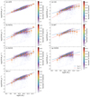 |
Fig. C.2. Same as Fig. C.1, but for galaxies at 0.72 ≤ z < 0.85. |
| In the text | |
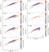 |
Fig. C.3. Same as Fig. C.1 but for galaxies at 0.85 ≤ z < 1.20. |
| In the text | |
Current usage metrics show cumulative count of Article Views (full-text article views including HTML views, PDF and ePub downloads, according to the available data) and Abstracts Views on Vision4Press platform.
Data correspond to usage on the plateform after 2015. The current usage metrics is available 48-96 hours after online publication and is updated daily on week days.
Initial download of the metrics may take a while.