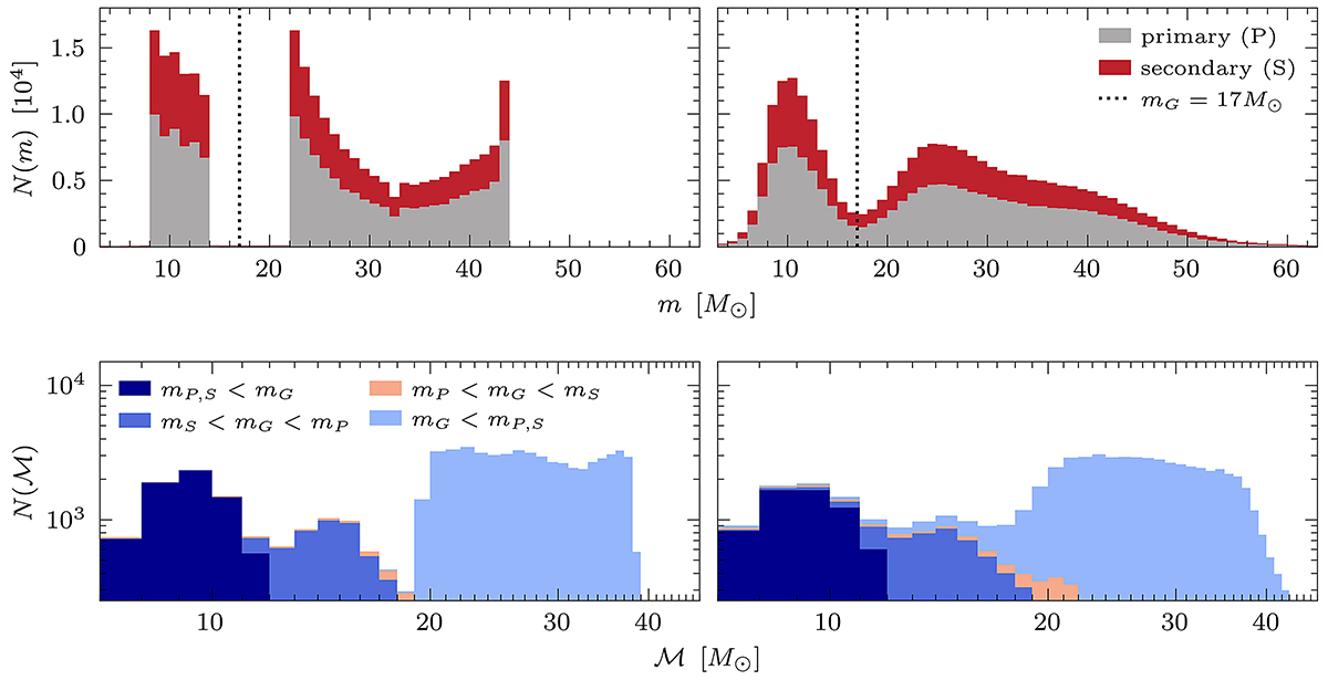
Fig. 4.
Download original image
BBH mass distribution resulting from our estimation, where we simulate approximately N = 1.2 × 10⁶ binaries and set η = 0.5 and ζ = 0.5. The latter means that half of the binaries follow the case A/B remnant function, and the other half follow the case C remnant curve (as shown in Fig. 2). The top row shows the resulting mass distribution of the individual primary (red) and secondary (grey) masses, in a stacked histogram with a bin-width of 1 M⊙. The bottom row shows the chirp mass distribution in a similar histogram, where we distinguish between four possible configurations of the primary and secondary mass with respect to the central value of the mass gap (mG): either both BHs are below the gap (dark blue), the secondary is below the gap while the primary is above it (blue) or vice versa (beige), or both are above the gap (light blue). The left column shows the exact results of our estimation, while the right column adds a Gaussian uncertainty to the results in order to make the simulated distribution look more similar to the observed one (as shown in Fig. 1). We based the Gaussian uncertainty on the average standard deviations of the GW data, as described in Appendix D.
Current usage metrics show cumulative count of Article Views (full-text article views including HTML views, PDF and ePub downloads, according to the available data) and Abstracts Views on Vision4Press platform.
Data correspond to usage on the plateform after 2015. The current usage metrics is available 48-96 hours after online publication and is updated daily on week days.
Initial download of the metrics may take a while.