| Issue |
A&A
Volume 674, June 2023
|
|
|---|---|---|
| Article Number | A201 | |
| Number of page(s) | 8 | |
| Section | Atomic, molecular, and nuclear data | |
| DOI | https://doi.org/10.1051/0004-6361/202244598 | |
| Published online | 23 June 2023 | |
Elastic and electron capture processes in slow He+–He collision★
1
School of Physics, Beijing Institute of Technology,
Beijing
100081, PR China
2
Faculty of foundation, Space Engineering University,
Beijing
101416, PR China
3
Institute of Applied Physics and Computational Mathematics,
Beijing
100088, PR China
e-mail: This email address is being protected from spambots. You need JavaScript enabled to view it.
; This email address is being protected from spambots. You need JavaScript enabled to view it.
4
HEDPS, Center for Applied Physics and Technology, Peking University,
Beijing
100084, PR China
Received:
26
July
2022
Accepted:
19
April
2023
Abstract
Aims. The elastic and electron-capture processes of He+ ions with ground helium atoms are very important for studies in astrophysics. It is essential to have reliable state-selective charge transfer, elastic, and transport cross-sections, along with the corresponding reaction rate coefficient data, especially for low collision energies.
Methods. We investigated the elastic and non-radiative electron-capture processes in He+(1s)–He(1s2) collisions are investigated employing the full quantum-mechanical molecular orbital close-coupling method. The adopted ab initio adiabatic potentials and coupling matrix elements were obtained by a multi-reference single- and double-excitation configuration interaction approach.
Results. We computed the elastic, charge-transfer, and transport cross-sections in the energy range of 0.01–2500eVamu−1 and the reaction rate coefficient in the temperature range of 10–109 K. Good agreement was achieved when compared to the available experimental and theoretical results. Shape resonance, Regge, and Glory oscillations were also found in the elastic and charge transfer cross-sections in the energy region considered here.
Key words: astroparticle physics / atomic processes / atomic data
Tables of the cross-sections and the corresponding reaction rate coefficient data are only available at the CDS via anonymous ftp to cdsarc.cds.unistra.fr (130.79.128.5) or via https://cdsarc.cds.unistra.fr/viz-bin/cat/J/A+A/674/A201
© The Authors 2023
 Open Access article, published by EDP Sciences, under the terms of the Creative Commons Attribution License (https://creativecommons.org/licenses/by/4.0), which permits unrestricted use, distribution, and reproduction in any medium, provided the original work is properly cited.
This article is published in open access under the Subscribe to Open model. This email address is being protected from spambots. You need JavaScript enabled to view it. to support open access publication.
1 Introduction
Charge transfer is an important process to consider in the modeling of X-ray emission in many astrophysical environments, which has been identified as one of the main sources of X-ray background. For example, it occurs during collisions of the solar wind (SW) ions with the neutral atmosphere in the heliosphere (Cox 1998; Cravens et al. 2001), as well as with planets (Wargelin et al. 2004), the geocorona (Robertson & Cravens 2003a,b), and comets (Lisse et al. 1996). When charge transfer occurs, the resulting solar wind ions are left in an excited state and the excited electron(s) then cascade to the ground state, generating a range of emission lines. Generally, X-rays can be used to measure the speed (Bodewits et al. 2004), composition (Kharchenko et al. 2003), and source region (Bodewits et al. 2007) of the solar wind and the bulk components of celestial atmospheres (Mullen et al. 2017). Overall, 8% of the elements in the solar wind are helium (Cravens 2002) and when α particles react with the neutral atmosphere, they produce a mixture of He2+, He+, and He. For example, in the study of diagnosing the atmosphere of comet 67P/Churyumov-Gerasimenko, Wedlund et al. (2016, 2019) pointed out that He+ ions mainly come from the charge exchange between the α particles in the solar wind and the neutral atmosphere of the comet. These mixed ions will further interact with the neutral atmosphere and result in a charge-exchange process.
Interstellar neutral helium is also of particular interest due to its large mean-free path for charge-exchange collisions with other atoms and molecules. The typical collisions between neutral He atom and He+ occur in the outer heliosheath in the low-energy region (0.1–10 eV). As shown in Fig. 2 of their paper, Scherer et al. (2014) considered that the He + He+→He+ +He process is the dominant process for CX with H and He in the outer heliosheath at such low energies. The Lyα absorption spectra provide a unique method for heliospheric and astrospheric diagnostics (Wood et al. 2005). Wood et al. (2007) predicted the Lyα absorption observations of the heliosphere and compared with actual Lyα spectra from the Hubble Space Telescope. They found that the charge transfer between interstellar hydrogen and protons can build hydrogen walls beyond the heliosphere. The hydrogen walls provide observational basis for measuring stellar mass-loss rates. Linsky & Wood (2014) proposed a new way to understand the relation of the stellar mass-loss rates of F-M dwarf stars with the X-ray emissions which based on the hydrogen wall. Scherer et al. (2014) have pointed out that the charge exchange processes of He+–He, He2+–He, and He+–He+ are very important for the study of astrospheres. This is due to the fact that the hydrogen walls are built in the interstellar medium and can be used to determine the stellar wind and interstellar parameters of some stars. However, the temperature in the interstellar medium is below 104 K, and at such low energies, the electron capture cross-sections for the above collision systems are very large, which may result in a helium wall. Therefore, the collisions of helium ions with neutral helium atoms are very important for the investigation of the astrophysical environment, and the contribution from the collisions involving He atoms and Heq+ ions cannot be neglected.
The collision processes between He+ and He atom have been extensively studied in the past. Experimental studies for the He+–He collision system mainly focus on the intermediate-and high energy region (>3 keVamu−1), total and state-selective charge-transfer cross-sections (Samaddar et al. 2020; Guo et al. 2017; Kamiński et al. 2013; Novikov 2010; Schöffler et al. 2009; Mančev 2007; Forest et al. 1995; Atan et al. 1991), and electron-loss and ionization cross-sections (Baxter et al. 2017; Ding et al. 2012; Santos et al. 2001, 2011; Miraglia & Gravielle 2010; Shevelko et al. 2009; Forest et al. 1995; Atan et al. 1991; de Castro Faria et al. 1988) have been measured and reported. However, the experiments in the low-energy region of this collision system are very limited, especially with regard to the state-selective charge-transfer cross-sections. As far as we know, only total electron capture cross-sections for this collision system have been measured by Hinds & Novick (1978), Hegerberg et al. (1978), Helm (1977), and Hayden & Utterback (1964) in the low-energy region. State-selective charge transfer cross-sections measurement have been performed by Wolterbeek & De Heer (1970) and Okasaka et al. (1994) with an energy region only down to about 1.5 keVamu−1 and 1 keVamu−1, respectively. On the theoretical side, cross-section calculations for He+−He collisions are also very scarce in the low-energy region.
Furthermore, there are no available state-selective chargetransfer cross-sections published in the energy region below 0.2 keVamu−1 as of yet. The calculations of electron capture cross-section for He+−He collisions have been performed by the TC-AOCC method and the SC-AOCC method in the energy region of 0.2−100 keVamu−1 (Zhao et al. 2018) and 1−225 keV amu−1 (Gao et al. 2018), respectively. However, due to the straight-line trajectory approximation of the nuclear motion applied in the semi-classical TC-AOCC method, it results in inherent limitations of TC-AOCC in describing the collision dynamics at very low energies below ~ 1 keVamu−1. On the other hand, compared with the full quantum QMOCC calculations, the inadequate consideration of the electronic correlations using the one-electron potential model also makes the TC-AOCC calculations inaccurate in treating many-electron target collisions for low energies below ~1 keV amu−1. Theoretical studies have also been conducted for the He+−He system by employing the JWKB semi-classical approximation (Barata & Conde 2010), the impact-parameter and close-coupling (CC) method (Sakabe & Izawa 1992), and the two-state asymptotic molecular orbital (2SasMO) methods (Hodgkinson & Briggs 1976) to calculate the total charge transfer cross-section. We would like to note that in all the above theoretical studies, only two ground states (2-state case) of the molecular ion were included in the calculations. Data on elastic cross-sections, transport cross-sections, and reaction rate coefficient related to the low-energy region are also very scarce in He+−He collisions.
In this paper, we carry out a theoretical study of the elastic and charge transfer processes of:
 (1a)
(1a)
 (1b)
(1b)
 (1c)
(1c)
where EL, GT, and ET correspond to elastic scattering, ground-state transfer (or resonant charge transfer) and transfer to excited states, respectively. The collision dynamics of the He+−He(1s2) system will be studied with the fully quantum-mechanical molecular orbital close-coupling (QMOCC) method, which is believed to be one of the most sophisticated methods in treating low-energy ion-atom and ion-molecule collisions. High-precision electron-capture cross-section data can be obtained, especially for energies lower than ~ 1 keVamu−1, since both the nuclear and electrons are treated quantally in the QMOCC method. The molecular structure data required in the QMOCC calculations have been obtained by employing the multi-reference single- and double-excitation configuration interaction (MRD-CI) method (Buenker & Phillips 1985; Stefan et al. 1995). Total and state-selective cross-sections are calculated in the present work. Meanwhile, the elastic and transport (diffusion and viscous) cross-sections are also presented and compared with other theoretical and experimental data. The main motivation of the present work is to generate accurate charge-transfer, elastic, transport cross-sections, and reaction rate coefficient for this collision system in the low-energy region by using a large MO expansion basis in the QMOCC method.
The present paper is organized as follows. In Sect. 2, we briefly outline the MRD-CI and QMOCC methods used in our calculations. In Sect. 3, we present and discuss the results of the cross-sections for the charge transfer, elastic, and transfer processes, as well as the reaction rate coefficient. In Sect. 4, we provie our conclusions. Atomic units are used throughout, unless otherwise stated.
2 Theoretical methods
2.1 QMOCC method
The basic technique of the QMOCC method for ion-atom collisions is outlined below (for a more detailed description, see. Zygelman et al. 1992; Bransden et al. 1993; Nolte et al. 2012). By solving a set of second-order radial coupled differential equations based on the perturbed stationary state model (PSS; Heil et al. 1981; Zygelman et al. 1992; Bransden et al. 1993) through the multichannel log-derivative algorithm (Johnson 1973), we can obtain the K matrix. Then the S matrix can be obtained as follows:
 (2)
(2)
As the coupling matrix elements for radial and rotational motion in the adiabatic representation undergo sharp changes near the avoided crossing, it can lead to numerical difficulties in integration of the QMOCC equation. Therefore, a unitary transformation is generally used to convert the electronic state from adiabatic representation into a diabatic representation (Zygelman et al. 1992). This transformation ensures that the coupling matrix element changes smoothly or becomes zero. In the case of He+ + He, which is a symmetric system composed of two identical nuclei, the electron wave function has two forms: gerade (g) and ungerade (u), and they are dynamically decoupled. Therefore, it is necessary to solve the QMOCC equations separately for each of these two forms of states. The radial function of the neutral channel matches the boundary conditions of the plane wave. For the channel with a Coulomb interaction, the asymptotic form can be changed to the Coulomb wave. The S matrix can be obtained from the K matrix. Under the same symmetry (g or u), the S matrix from channel i to channel j has the same representation. Similarly, the scattering amplitude of transitions also takes a standard form (Bransden et al. 1993):
 (3)
(3)
where ki represents the initial momentum of the center of mass, J is the quantum number of the total angular momentum, and PJ is the Legendre polynomial on the order of J. The differential cross-sections of elastic scattering and charge transfer processes are expressed as:
 (4)
(4)
respectively, where the S matrix accounting for the identity of the colliding particles is given by:
![Mathematical equation: $S_{ij,J}^{{\rm{el}}}\left( {E,\theta } \right) = {1 \over 2}\left[ {S_{ij,J}^g + S_{ij,J}^u} \right],$](/articles/aa/full_html/2023/06/aa44598-22/aa44598-22-eq7.png) (5a)
(5a)
![Mathematical equation: $S_{ij,J}^{{\rm{ex}}}\left( {E,\theta } \right) = {1 \over 2}\left[ {S_{ij,J}^g - S_{ij,J}^u} \right],$](/articles/aa/full_html/2023/06/aa44598-22/aa44598-22-eq8.png) (5b)
(5b)
where the superscript el and ex in Eq. (4) represent the elastic scattering and charge transfer processes, respectively. Integrating Eq. (4) obtains the integral cross-sections for the elastic and charge transfer processes over the entire solid angle of scattering Ω:
 (6a)
(6a)
 (6b)
(6b)
In addition, Eq. (1b) represents the resonant charge transfer process. Cross-sections for this resonant charge transfer process can be approximately obtained from the scattering phase difference between the g level and the u level as:
 (7)
(7)
where η is the phase shift, and the relationship between the η and S matrix under the symmetry of g and u can be expressed as:
 (8)
(8)
For a symmetric ion-atom system, integral elastic total cross-sections and transport (diffusion and viscous) cross-sections can be obtained by analytically integrating the scattering angle. They have a unified form:
 (9)
(9)
where + and – represent even and odd values of J, and the corresponding coefficients are given in Table 1. The elastic integral total cross-sections are the summation of the elastic and charge transfer cross-sections (Krstić & Schultz 1999).
2.2 Molecular structure calculations
The adiabatic potential energy curves and coupling matrix elements for radial and rotational processes have been calculated by the ab initio MRD-CI package (Buenker & Phillips 1985; Stefan et al. 1995). The helium atom was described by the correlation-consistent, polarization valence, quadruple-ζ (cc-pVQZ) type basis set (Dunning & Thom 1989) with a diffuse (2s3p2d) set. The final contraction basis set was (12s, 6p, 4d)/[6s, 6p, 4d]. Configurations of  were selected using a threshold set at 10−8 hartree and internuclear distances of R = 0.6–60 au. The MRD-CI package was used to calculate the lowest two states, which includes eleven
  , eleven
  , six 2Πg, and six 2Πu states of the
  molecule ion. The electron wave function has gerade (g) and ungerade (u) manifolds due to the interchange of the two identical nuclei. Table 2 shows the energy levels of the asymptotic atomic states of the
  molecule ion. The relative errors between our calculated energies and the experimental data (Morton et al. 2006) were smaller than 0.059 eV in the asymptotic region.
In order to validate the accuracy of the molecular ion’s structure in this study, we also calculated the values of the equilibrium nuclear distance, Re, and potential well depth, De, for the two ground states of  molecular ion and compared them with other available theoretical data. Table 3 shows that the present spectral constants for the ground state of
  molecular ion are reliable.
The adiabatic potential energy curves of the molecular ion are calculated and shown in Fig. 1.  and
and  correspond to the configurations at the dissociation limit (R = ∞): [He+(1s) + He(1s2)] and [He(1s2) + He+(1s)], respectively, representing the initial channel of the He+(1s)–He(1s2) collision system. We can see from Fig. 1 that when R < 3 au, a series of dense avoided crossings are formed among the excited states of the molecular ion with the same symmetry. These complex avoided crossings show a very complicated electron trapping mechanism, which should be important in the collision dynamics. However, due to the large energy difference between the incident channel and its above channels (such as the energy difference between the incident channel He(1s2 1S) + He+(1s 2S) and the channel He+(1s 2S) + He(1s2s 1S) at the dissociation limit is 19.82 eV), when the relative energy of the collision is lower than 9.91eVamu−1 (19.82 eV divided by the reduced mass of the collision system
  in atomic mass units), the charge transfer process between these two reaction channels cannot occur. It can be expected that the resonant charge transfer between the two ground states
  and
and  will be the dominant process in He+(1s)–He(1s2) collision at low energies.
Figure 2 shows the radial coupling matrix element of  containing ETF correction (Errea et al. 1982), which determines the transition between states with the same spin and the same spatial symmetry. A series of radial couplings can be seen in the region of R < 3.0 au, i.e.,
  , etc. According to the “hidden crossing” theory (Janev 1997), these couplings will last until n → ∞, which will promote the system to reach the ionization limit in the collision approach stage. The position of these peaks in the radial coupling matrix element are consistent with the positions where the avoided crossings of the adiabatic potential energy are observed in Fig. 1. As mentioned earlier, due to the large energy level difference between the incident channel and other channels, it can be observed that the
  coupling is weak in the whole R range, while the
  coupling is only strong at R = 1.4 au, which may play an important role in the charge transfer process in regions characterized by higher collision energy.
Figure 3 shows the rotational coupling matrix elements of the He2+ molecular ion with ETF correction. These couplings determine the transition between states with the same spin but different spatial symmetry. Notably, it is evident that there are jumps in some rotational coupling matrix elements at small inter-nuclear distances, such as at R = 1.4 au (in Fig. 3b1), which arise from strong avoided crossings between the potential energy curves of Σ state under adiabatic representation. However, in dia-batic representation, these rotational coupling matrix elements become smooth.
Asymptotic atomic energies for the  molecular ion states.
Values of equilibrium position Re (au) and depth of potential well De (eV) for the lowest two states of  molecular ion.
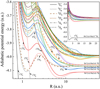 |
Fig. 1 Curves of adiabatic potential energy of the |


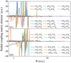 |
Fig. 2 Adiabatic coupling matrix elements for radial process among the ɡ-states(a1) and among the u-states(a2) of |

3 Results and discussion
3.1 Charge-transfer cross-sections
The total charge-transfer cross-sections for the He+(1s)−He(1s2) system are shown in Fig. 4, over the energy range of 0.01−2500 eV amu−1. The results are compared with those from previous studies, including the AOCC calculations of Gao et al. (2018) and Zhao et al. (2018), the CC results of Sakabe & Izawa (1991), the JWKB results of Barata & Conde (2010), and the results of the two-state asymptotic MO (2SasMO) method of Hodgkinson & Briggs (1976). To obtain convergent results, the present QMOCC calculations consider the 2 (lowest) states ( and
and  ) and 34 states (
 , and l−62∏u), respectively. The comparison indicates that the contribution of transfer to the excited state process is negligible compared to the resonance charge transfer process. Compared with the AOCC calculations of Zhao et al. (2018), Gao et al. (2018), and the JWKB results from Barata & Conde (2010), the present QMOCC results show excellent agreement with the available experimental (Hayden & Utterback 1964; Helm 1977; Hinds & Novick 1978; Hegerberg et al. 1978) and theoretical results (Sakabe & Izawa 1991; Barata & Conde 2010) for incident energy less than about 10 eV amu−1; however, discrepancies appear for higher energies. This difference may be attributed to the fact that quantum effects become important at very low incident energies and the CC and JWKB treatments become unreliable. Moreover, the energy range of 0.01−0.45 eVamu−1 exhibits rich oscillation structures, which have been identified as Regge oscillations and shape resonances in charge transfer, elastic and momentum transfer cross-sections for H+−H (Wu et al. 2010) and H+ with inert gases collisions (Ovchinnikov et al. 2006). Regge oscillations can be determined with the poles of the S matrix (the so-called Regge poles), which correspond to resonances associated with potential barriers formed by the attractive polarization and exchange potentials and the repulsive centrifugal potentials (Krstić et al. 2004). Regge oscillations are a general feature of resonant charge transfer processes in atom-ion collisions.
The present study shows the total cross-sections for ET and GT processes in He+ +He(1s2) collisions in Fig. 5. Additionally, the spin-resolved cross-sections for electron capture to triplet (He+ +He(1s2) → He(lsnl 3L) + He+ n ≥ 2) and singlet states (He+ + He(1s2) → He(lsnl 1L) + He+ n ≥ 2) of He atoms are provided as the ET triplet and ET singlet, respectively. For comparison, the SC-AOCC results from Gao et al. (2018) and experimental data from Guo et al. (2017) are also presented. As mentioned previously, only the GT process can occur when the collision energy is below 9.91 eV amu−1. All reaction channels, including the ET process, are available in the energy region above 12 eV amu−1. From Fig. 5, it is evident that the GT process dominates the considered energy range, and the cross-section decreases with the increase of collision energy. However, the ET cross-sections increase with increasing collision energy. It is worth noting that GT cross-sections are in good agreement with the theoretical results of Gao et al. (2018) in the overlapping energy region. In contrast, for sub-dominant charge transfer channels, the present cross-sections are smaller than those of SC-AOCC results of Gao et al. (2018). The discrepancy between the present results and the previous SC-AOCC calculations in the energy range above 1000 eV amu−1 originates from the difference in the size of expansion bases. Specifically, in SC-AOCC calculations from Gao et al. (2018), 1260 atomic states in AO bases are included, whereas only 32 molecular states are considered in our calculations. It is important to note that the experimental data of Guo et al. (2017) are significantly lower than the SC-AOCC results of Gao et al. (2018) at a collision energy of about 7.5 keV amu−1.
The QMOCC method was used to calculate the state-selective cross-sections. Figure 6 shows our results for charge transfer to 1snl (n = 2,3; l = 0,1,2) shells of the He atom, which are compared with the TC-AOCC calculations of Zhao et al. (2018). The resonant charge transfer cross-sections in our present work are in good agreement with the theoretical results of Zhao et al. (2018). However, the cross-sections for charge transfer to the excited states of the He atom are quite different in the overlapping energy region. This disagreement may be due to the different size of the expansion basis of MO and AO bases employed in QMOCC and TC-AOCC methods, as well as the neglect of electronic correlation in the TC-AOCC method Zhao et al. (2018). The latter aspect is particularly significant for low-energy collisions.
In addition to nl-resolved cross-sections, we also calculated the spin-resolved state-selective charge transfer cross-sections for the He+−He collision system. Figure 7 shows our QMOCC cross-sections for charge transfer to the singlet and triplet states of the He(lsnl, n = 2,3) atom in He+−He collisions, respectively, and compares them with the first Born approximation results of Winter & Lin (1975), semi-classical approximation results of Hildenbrand et al. (1995), SC-AOCC results of Gao et al. (2018), impact parameter results of Sural et al. (1967), and experimental data of Okasaka et al. (1994), Hippler et al. (1978), and Wolterbeek & De Heer (1970). From this figure, we can observe that the magnitudes of these sub-dominant charge transfer cross-sections are considerably lower than those of the dominant channel (as shown in Fig. 5). From Figs. 7b and c, we can see that the values of all theoretical cross-sections for electron capture to the singlet and triplet states of the He(ls2s) atom have significant differences in the overlapping energy region. However, the present cross-sections for charge transfer to the singlet state of the He(1s2p) agree well with the other theoretical results in the overlapping energy range, as shown in Fig. 7a. Regarding the charge transfer to the He(ls3sl 1,3S) state (in Figs. 7d and e), we can see that the current cross-sections are in good agreement with the experimental data of Okasaka et al. (1994) and Wolterbeek & De Heer (1970) in the overlapping energy region. From Fig. 7d, we also note that for the cross-sections of charge transfer to the triplet state of He (1s3s), the present results are also in good agreement with the SC-AOCC results of Gao et al. (2018) in the overlapping energy range. For singlet states, the current results are slightly lower than those of Gao et al. (2018).
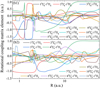 |
Fig. 3 Adiabatic coupling matrix elements for rotational process among the ɡ-states(b1) and among the u-states(b2) of |

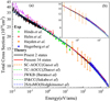 |
Fig. 4 Total cross-sections for electron capture process in He+(1s)−He(1s2) collision system obtained by the QMOCC method and compared with the experimental and theoretical data. Theory: results of the present study, with the 2-state case (black solid line) and 34-state case (red solid line), SC-AOCC results of Gao et al. (2018; orange dashed line), TC-AOCC results of Zhao et al. (2018; green dashed line), JWKB results of Barata & Conde (2010; pink dash-dotted line), CC results of Sakabe & Izawa (1991; green dash-dotted line), and 2SAsMO results of Hodgkinson & Briggs (1976; blue dash-dotted line). Experimental results: Hinds & Novick (1978; green filled diamond), Helm (1977; red filled circle), Hayden & Utterback (1964; orange filled inverse triangle), and Hegerberg et al. (1978; blue filled triangle). |
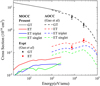 |
Fig. 5 Total cross-sections for ET and GT processes in He+(1 s)−He(1 s2) collisions as a function of collision energy. ET triplet (singlet) is the cross-sections for electron capture to the triplet (singlet) states of He(1snl). Results of the present study (solid line) and SC-AOCC results of Gao et al. (2018, dashed line). Experimental data of Guo et al. (2017) shown as black filled triangle for the GT process and red filled circles for the ET process. |
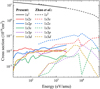 |
Fig. 6 State-selective cross-sections for electron capture to the He(1snl), n ≤ 3) states, compared with the TC-AOCC results of Zhao et al. (2018). |
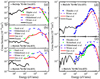 |
Fig. 7 Spin-resolved state-selective charge transfer cross-sections for electron capture to the singlet and triplet states of He(1snl, n = 2,3) atom in He+−He collision system. Theoretical: this study (black solid line), Gao et al. (2018; red solid line), Winter & Lin (1975; purple dashed line), (1995; blue dashed line), Sural et al. (1967; green dashed line); experimental: Okasaka et al. (1994; blue filled circle), Hippler et al. (1978; green filled diamond), and Wolterbeek & De Heer (1970; green filled triangle). |
3.2 Elastic and transport cross-sections
Figure 8 shows the total elastic integral cross-sections of the collision between a He+ ion and He atom for our present work and compares them with the results obtained from the JWKB method by Barata & Conde (2010) as well as the close-coupling method by Chicheportiche et al. (2013). As shown in the figure, our results are consistent with other theoretical results in the considered energy range. However, for energies lower than about 0.5 eV amu−1, noticeable discrepancies can be observed in comparison with our present QMOCC results and the close coupling calculations of Chicheportiche et al. (2013), and the discrepancy increases as the incident energy decreases. This difference is believed to be due to the different potential curves used in the close coupling calculations. Up to now, there has been no theoretical calculation or experimental measurement published for the pure elastic cross-section of this collision system. It is worth noting that the sum of elastic cross-sections represented by Eq. (6a) and the charge transfer cross-sections is nearly identical to the integral elastic total cross-sections represented by Eq. (9).
For the sake of convenience in related applications, we also calculated and presented the transport cross-sections, including the diffusion and viscosity cross-sections, for this collision system. Figure 9 shows our transport cross-sections and compares them with the results obtained from the close-coupling quantum method by Chicheportiche et al. (2013). No experimental data have been reported for the transport cross-sections of this collision system as of yet. The study by Chicheportiche et al. (2013) provides the only set of diffusion cross-section data (shown in Fig. 9). We observe that for energy levels above 0.3 eV amu−1, our resulting values are approximately 14% larger than those of Chicheportiche et al. (2013). Further experimental investigations are required to verify the accuracy of our results.
Similarly to the features observed in Fig. 4, rich oscillatory structures can also be found in the elastic and transport cross-sections in Figs. 8 and 9. Those located at incident energies less than 0.45 eV amu−1 are shape resonance and Regge oscillation. On the other hand, another type of oscillatory structures, glory oscillations, can be found for incident energies larger than 0.45 eV amu−1, which have not been observed in the electron capture cross-sections in Fig. 4. Glory oscillations mainly result from the presence of stationary phase in the summation of L partial waves in the elastic cross-sections. However, no stationary phase exists as a function of L partial waves in the diffusive cross-sections and, therefore, glory oscillations cannot be found in those (Krstić et al. 2004; Ovchinnikov et al. 2006).
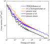 |
Fig. 8 Elastic and elastic integer total cross-sections (including elastic and charge transfer cross-sections) for He+(1s)−He(1s2) collisions and comparison with previous theoretical date(Barata & Conde 2010; Chicheportiche et al. 2013). Black solid line: elastic cross-sections calculated by Eq. (6a). Red solid line: elastic integer total cross-sections calculated by Eq. (9). Blue solid line: summation of resonant charge transfer cross-sections calculated by Eq. (7) and elastic cross-sections calculated by Eq. (6a). |
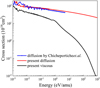 |
Fig. 9 Diffusion and viscous cross-sections for He+(1s)−He(1s2) collision system and comparison with previous theoretical data (Chicheportiche et al. 2013). |
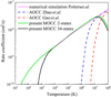 |
Fig. 10 Total reaction rate coefficients for He+(1s)−He(1s2) collisions. Solid line: results of this study. Dashed line: results based on the AOCC method by Zhao et al. (2018) and Gao et al. (2018). Short dotted line: results based on numerical simulations by Potters & Goedheer (1985). |
3.3 Reaction rate coefficients
By averaging our QMOCC cross-sections over Maxwell-Boltzmann velocity distributions, we obtained the charge transfer reaction rate coefficient in the temperature range of 10−109 K. Figure 10 shows the total reaction rate coefficients of the 2-state and 34-state cases, based on the QMOCC method and compares the results based on the AOCC method by Zhao et al. (2018) and Gao et al. (2018) and based on numerical simulation by Potters & Goedheer (1985). It can be found that our results are in good agreement with other theoretical results. The results of Zhao et al. (2018) and Gao et al. (2018) sharply decreased in the region below 107 K because the energy range they considered in the calculation was limited and the minimal value was only 200 eV amu−1. Similarly, our 34-state results are smaller than the 2-state results in the region by less than 104 K, and both results show a decreasing trend in the region greater than 107 K; the latter is also caused by the slightly smaller energy range considered in the calculation. Figure 11 shows nl-resolved charge transfer reaction rate coefficients for He+−He(1s) collision. Combined with Fig. 10, considering the limitation that the maximum energy in the present calculation is only 2500 eV amu−1, it can be estimated that the reaction rate coefficient of each charge transfer increases with the increase of temperature.
4 Conclusion
In this study, we investigated elastic and single-electron charge transfer processes for He+(1s)−He(1s2) collisions employing the QMOCC method in the energy range of 0.01−2500 eV amu−1. We performed 2-state and 34-state calculations and achieved a good agreement with existing theoretical and experimental results. The dominant state-selective cross-sections for charge transfer to the He(1s2) state are in perfect agreement with the results of Gao et al. (2018) in the overlapping energy region. And other state-selective cross-sections for sub-dominant channels can be smoothly connected with the results of Gao et al. (2018) in the overlapping energy region. However, the significant difference from the results of Zhao et al. (2018) is attributed to the fact that the electronic interaction is neglected in the one-electron treatment of Zhao et al. (2018), which is very important for low-energy collisions for multi-electron collision systems. We also provided spin-resolved state-selective charge transfer cross-sections and reaction rate coefficients for this collision system, filling a gap in the data for state-selective cross-sections and reaction rate coefficients in the low-energy collision region. In addition, we provide elastic and transport cross-sections, which may be useful for relevant plasma investigations. Our study also reveals the presence of shape resonance, Regge oscillations, and Glory oscillations in the charge transfer, along with elastic and transport cross-sections at different energy ranges. We discuss the corresponding physical mechanisms here as well. While the present QMOCC method is suitable for treating low-energy ion-atom and ion-molecule collisions (E ≤ ~5 keVamu−1), it faces computational limitations when treating highly excited states and continuum states channels, which require a consideration of a very high number of reaction channels to obtain convergent results in close-coupling calculations. In a future work, we plan to investigate electron-capture processes in collisions of Heq+(q = 0−2) with neutral atoms/molecules (e.g., O, OH, and CO2). We also plan to obtain and provide single- and double-electron-capture cross-sections, which stand as important atomic data required for related SWCX and cometary CX simulations.
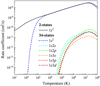 |
Fig. 11 nl-resolved charge transfer reaction rate coefficients for He+(1s)−He(1s2) collisions. |
Acknowledgements
This work was supported by the National Natural Science Foundation of China (Grants Nos. 11934004, 11774037 and 51735001) and the CRP project of International Atomic Energy Agency (No. 23196/R0).
References
- Atan, H., Steckelmacher, W., & Lucas, M. W. 1991, J. Phys. B: At. Mol. Opt. Phys., 24, 2559 [NASA ADS] [CrossRef] [Google Scholar]
- Barata, J., & Conde, C. 2010, Nucl. Instrum. Methods Phys. Res. A, 619, 21 [CrossRef] [Google Scholar]
- Baxter, M., Kirchner, T., & Engel, E. 2017, Phys. Rev. A, 96, 032708 [NASA ADS] [CrossRef] [Google Scholar]
- Bodewits, D., Juhsz, Z., Hoekstra, R., & Tielens, A. G. G. M. 2004, ApJ, 606, L81 [NASA ADS] [CrossRef] [Google Scholar]
- Bodewits, D., Christian, D. J., Torney, M., et al. 2007, A&A, 469, 1183 [NASA ADS] [CrossRef] [EDP Sciences] [Google Scholar]
- Bransden, B. H., Mcdowell, M., & Mansky, E. J. 1993, Phys. Today, 46, 124 [CrossRef] [Google Scholar]
- Buenker, R. J., & Phillips, R. A. 1985, J. Mol. Struct.: THEOCHEM, 123, 291 [CrossRef] [Google Scholar]
- Carrington, A., Pyne, C. H., & Knowles, P. J. 1995, J. Chem. Phys., 102, 5979 [NASA ADS] [CrossRef] [Google Scholar]
- Chicheportiche, A., Lepetit, B., Benhenni, M., Gadea, F. X., & Yousfi, M. 2013, J. Phys. B: At. Mol. Opt. Phys., 46, 065201 [NASA ADS] [CrossRef] [Google Scholar]
- Cox, D. P. 1998, The Local Bubble and Beyond Lyman-Spitzer-Colloquium (Springer Berlin Heidelberg), 121 [NASA ADS] [CrossRef] [Google Scholar]
- Cravens, T. E. 2002, Science, 296, 1042 [CrossRef] [Google Scholar]
- Cravens, T. E., Robertson, I. P., & Snowden, S. L. 2001, J. Geophys. Res. Space Phys., 106, 24883 [NASA ADS] [CrossRef] [Google Scholar]
- de Castro Faria, N. V., Freire, F. L., & de Pinho, A. G. 1988, Phys. Rev. A, 37, 280 [CrossRef] [Google Scholar]
- Ding, B., Li, H., & Zhang, W. 2012, Int. J. Mass Spectrom., 313, 41 [NASA ADS] [CrossRef] [Google Scholar]
- Dunning, & Thom, H. 1989, J. Chem. Phys., 90, 1007 [NASA ADS] [CrossRef] [Google Scholar]
- Errea, L. F., Mendez, L., & Riera, A. 1982, J. Phys. B: At. Mol. Phys., 15, 101 [NASA ADS] [CrossRef] [Google Scholar]
- Forest, J. L., Tanis, J. A., Ferguson, S. M., et al. 1995, Phys. Rev. A, 52, 350 [NASA ADS] [CrossRef] [Google Scholar]
- Gadea, F. X., & Paidarová, I. 1996, Chem. Phys., 209, 281 [NASA ADS] [CrossRef] [Google Scholar]
- Gao, J. W., Wu, Y., Wang, J. G., Sisourat, N., & Dubois, A. 2018, Phys. Rev. A, 97, 052709 [NASA ADS] [CrossRef] [Google Scholar]
- Guo, D. L., Ma, X., Zhang, R. T., et al. 2017, Phys. Rev. A, 95, 012707 [NASA ADS] [CrossRef] [Google Scholar]
- Hayden, H. C., & Utterback, N. G. 1964, Phys. Rev., 135, A1575 [NASA ADS] [CrossRef] [Google Scholar]
- Hegerberg, R., Stefansson, T., & Elford, M. T. 1978, J. Phys. B: At. Mol. Phys., 11, 133 [NASA ADS] [CrossRef] [Google Scholar]
- Heil, T. G., Butler, S. E., & Dalgarno, A. 1981, Phys. Rev. A, 23, 1100 [NASA ADS] [CrossRef] [Google Scholar]
- Helm, H. 1977, J. Phys. B: At. Mol. Phys., 10, 3683 [NASA ADS] [CrossRef] [Google Scholar]
- Hildenbrand, R., Grun, N., & Scheid, W. 1995, J. Phys. B: At. Mol. Opt. Phys., 28, 4781 [NASA ADS] [CrossRef] [Google Scholar]
- Hinds, E. A., & Novick, R. 1978, J. Phys. B: At. Mol. Phys., 11, 2201 [NASA ADS] [CrossRef] [Google Scholar]
- Hippler, R., Schartner, K. H., & Beyer, H. F. 1978, J. Phys. B: At. Mol. Phys., 11, L337 [NASA ADS] [CrossRef] [Google Scholar]
- Hodgkinson, D. P., & Briggs, J. S. 1976, J. Phys. B: At. Mol. Phys., 9, 255 [NASA ADS] [CrossRef] [Google Scholar]
- Janev, R. 1997, Nucl. Instrum. Methods Phys. Res. B, 124, 290 [CrossRef] [Google Scholar]
- Johnson, B. 1973, J. Comput. Phys., 13, 445 [NASA ADS] [CrossRef] [Google Scholar]
- Kamiński, P., Drozdowski, R., & Oppen, G. 2013, Eur. Phys. J. Special Top., 222, 2293 [CrossRef] [Google Scholar]
- Kharchenko, V., Rigazio, M., Dalgarno, A., & Krasnopolsky, V. A. 2003, ApJ, 585, L73 [NASA ADS] [CrossRef] [Google Scholar]
- Krstić, P. S., & Schultz, D. R. 1999, Phys. Rev. A, 60, 2118 [CrossRef] [Google Scholar]
- Krstić, P. S., Macek, J. H., Ovchinnikov, S. Y., & Schultz, D. R. 2004, Phys. Rev. A, 70, 042711 [CrossRef] [Google Scholar]
- Lee, E. P. F. 1993, J. Chem. Soc., Faraday Trans., 89, 645 [CrossRef] [Google Scholar]
- Linsky, J. L., & Wood, B. E. 2014, ASTRA Proc., 1, 43 [NASA ADS] [CrossRef] [Google Scholar]
- Lisse, C. M., & Dennerl, K. 1996, Science, 274, 205 [NASA ADS] [CrossRef] [Google Scholar]
- Mančev, I. 2007, Phys. Rev. A, 75, 052716 [CrossRef] [Google Scholar]
- Miraglia, J. E., & Gravielle, M. S. 2010, Phys. Rev. A, 81, 042709 [NASA ADS] [CrossRef] [Google Scholar]
- Morton, D. C., Wu, Q., & Drake, G. 2006, Can. J. Phys., 84 [Google Scholar]
- Mullen, P. D., Cumbee, R. S., Lyons, D., et al. 2017, ApJ, 844, 7 [NASA ADS] [CrossRef] [Google Scholar]
- Nolte, J. L., Stancil, P. C., Liebermann, H. P., et al. 2012, J. Phys. B: At. Mol. Opt. Phys., 45, 245202 [NASA ADS] [CrossRef] [Google Scholar]
- Novikov, N. V. 2010, J. Surf. Invest. , 4, 276 [CrossRef] [Google Scholar]
- Okasaka, R., Kawabe, K., Kawamoto, S., et al. 1994, Phys. Rev. A, 49, 246 [NASA ADS] [CrossRef] [Google Scholar]
- Ovchinnikov, S. Y., Krstić, P. S., & Macek, J. H. 2006, Phys. Rev. A, 74, 042706 [NASA ADS] [CrossRef] [Google Scholar]
- Potters, J., & Goedheer, W. 1985, Nuclear Fusion, 25, 779 [CrossRef] [Google Scholar]
- Robertson, I. P., & Cravens, T. E. 2003a, Geophys. Res. Lett., 30 [Google Scholar]
- Robertson, I. P., & Cravens, T. E. 2003b, J. Geophys. Res.: Space Phys., 108, A10 [NASA ADS] [CrossRef] [Google Scholar]
- Sakabe, S., & Izawa, Y. 1991, At. Data Nuclear Data Tables, 49, 257 [NASA ADS] [CrossRef] [Google Scholar]
- Sakabe, S., & Izawa, Y. 1992, Phys. Rev. A, 46, 1704 [NASA ADS] [CrossRef] [Google Scholar]
- Samaddar, S., Jana, D., Purkait, K., & Purkait, M. 2020, J. Phys. B: At. Mol. Opt. Phys., 53, 245202 [NASA ADS] [CrossRef] [Google Scholar]
- Santos, A. C. F., Melo, W. S., Sant’Anna, M. M., Sigaud, G. M., & Montenegro, E. C. 2001, Phys. Rev. A, 63, 062717 [NASA ADS] [CrossRef] [Google Scholar]
- Santos, A. C. F., Sigaud, G. M., Melo, W. S., Sant’Anna, M. M., & Montenegro, E. C. 2011, J. Phys. B: At. Mol. Opt. Phys., 44, 045202 [NASA ADS] [CrossRef] [Google Scholar]
- Scherer, K., Fichtner, H., Fahr, H.-J., Bzowski, M., & Ferreira, S. E. S. 2014, A&A, 563, A69 [NASA ADS] [CrossRef] [EDP Sciences] [Google Scholar]
- Schöffler, M. S., Titze, J., Schmidt, L. P. H., et al. 2009, Phys. Rev. A, 79, 064701 [CrossRef] [Google Scholar]
- Shevelko, V., Kato, D., Song, M.-Y., et al. 2009, Nucl. Instrum. Methods Phys. Res. B: Beam Interact. Mater. Atoms, 267, 3395 [CrossRef] [Google Scholar]
- Stefan, Krebs, Robert, J., & Buenker 1995, J. Chem. Phys., 103, 5613 [NASA ADS] [CrossRef] [Google Scholar]
- Sural, D. P., Mukherjee, S. C., & Sil, N. C. 1967, Phys. Rev., 164, 156 [NASA ADS] [CrossRef] [Google Scholar]
- Wargelin, B. J., Markevitch, M., Juda, M., et al. 2004, ApJ, 607, 596 [Google Scholar]
- Wedlund, C. S., Kallio, E., Alho, M., Nilsson, H., & Gronoff, G. 2016, A&A, 587, A154 [NASA ADS] [CrossRef] [EDP Sciences] [Google Scholar]
- Wedlund, C. S., Behar, E., Kallio, E., et al. 2019, A&A, 630, A36 [NASA ADS] [CrossRef] [EDP Sciences] [Google Scholar]
- Winter, T. G., & Lin, C. C. 1975, Phys. Rev. A, 12, 434 [NASA ADS] [CrossRef] [Google Scholar]
- Wolterbeek, L., & De Heer, F. J. 1970, Physica, 48, 345 [NASA ADS] [CrossRef] [Google Scholar]
- Wood, B. E., Redfield, S., Linsky, J. L., Müller, H.-R., & Zank, G. P. 2005, ApJS, 159, 118 [Google Scholar]
- Wood, B. E., Izmodenov, V. V., Linsky, J. L., & Alexashov, D. 2007, ApJ, 659, 1784 [NASA ADS] [CrossRef] [Google Scholar]
- Wu, Y., Wang, J. G., Krstić, P. S., & Janev, R. K. 2010, J. Phys. B: At. Mol. Opt. Phys., 43, 201003 [NASA ADS] [CrossRef] [Google Scholar]
- Zhao, G. P., Liu, L., Chang, Z., Wang, J. G., & Janev, R. K. 2018, J. Phys. B: At. Mol. Opt. Phys., 51, 085201 [NASA ADS] [CrossRef] [Google Scholar]
- Zygelman, B., Cooper, D. L., Ford, M. J., et al. 1992, Phys. Rev. A, 46, 3846 [NASA ADS] [CrossRef] [Google Scholar]
All Tables
Values of equilibrium position Re (au) and depth of potential well De (eV) for the lowest two states of molecular ion.
All Figures
|
Fig. 1 Curves of adiabatic potential energy of the |
| In the text | |
|
Fig. 2 Adiabatic coupling matrix elements for radial process among the ɡ-states(a1) and among the u-states(a2) of |
| In the text | |
|
Fig. 3 Adiabatic coupling matrix elements for rotational process among the ɡ-states(b1) and among the u-states(b2) of |
| In the text | |
|
Fig. 4 Total cross-sections for electron capture process in He+(1s)−He(1s2) collision system obtained by the QMOCC method and compared with the experimental and theoretical data. Theory: results of the present study, with the 2-state case (black solid line) and 34-state case (red solid line), SC-AOCC results of Gao et al. (2018; orange dashed line), TC-AOCC results of Zhao et al. (2018; green dashed line), JWKB results of Barata & Conde (2010; pink dash-dotted line), CC results of Sakabe & Izawa (1991; green dash-dotted line), and 2SAsMO results of Hodgkinson & Briggs (1976; blue dash-dotted line). Experimental results: Hinds & Novick (1978; green filled diamond), Helm (1977; red filled circle), Hayden & Utterback (1964; orange filled inverse triangle), and Hegerberg et al. (1978; blue filled triangle). |
| In the text | |
|
Fig. 5 Total cross-sections for ET and GT processes in He+(1 s)−He(1 s2) collisions as a function of collision energy. ET triplet (singlet) is the cross-sections for electron capture to the triplet (singlet) states of He(1snl). Results of the present study (solid line) and SC-AOCC results of Gao et al. (2018, dashed line). Experimental data of Guo et al. (2017) shown as black filled triangle for the GT process and red filled circles for the ET process. |
| In the text | |
|
Fig. 6 State-selective cross-sections for electron capture to the He(1snl), n ≤ 3) states, compared with the TC-AOCC results of Zhao et al. (2018). |
| In the text | |
|
Fig. 7 Spin-resolved state-selective charge transfer cross-sections for electron capture to the singlet and triplet states of He(1snl, n = 2,3) atom in He+−He collision system. Theoretical: this study (black solid line), Gao et al. (2018; red solid line), Winter & Lin (1975; purple dashed line), (1995; blue dashed line), Sural et al. (1967; green dashed line); experimental: Okasaka et al. (1994; blue filled circle), Hippler et al. (1978; green filled diamond), and Wolterbeek & De Heer (1970; green filled triangle). |
| In the text | |
|
Fig. 8 Elastic and elastic integer total cross-sections (including elastic and charge transfer cross-sections) for He+(1s)−He(1s2) collisions and comparison with previous theoretical date(Barata & Conde 2010; Chicheportiche et al. 2013). Black solid line: elastic cross-sections calculated by Eq. (6a). Red solid line: elastic integer total cross-sections calculated by Eq. (9). Blue solid line: summation of resonant charge transfer cross-sections calculated by Eq. (7) and elastic cross-sections calculated by Eq. (6a). |
| In the text | |
|
Fig. 9 Diffusion and viscous cross-sections for He+(1s)−He(1s2) collision system and comparison with previous theoretical data (Chicheportiche et al. 2013). |
| In the text | |
|
Fig. 10 Total reaction rate coefficients for He+(1s)−He(1s2) collisions. Solid line: results of this study. Dashed line: results based on the AOCC method by Zhao et al. (2018) and Gao et al. (2018). Short dotted line: results based on numerical simulations by Potters & Goedheer (1985). |
| In the text | |
|
Fig. 11 nl-resolved charge transfer reaction rate coefficients for He+(1s)−He(1s2) collisions. |
| In the text | |
Current usage metrics show cumulative count of Article Views (full-text article views including HTML views, PDF and ePub downloads, according to the available data) and Abstracts Views on Vision4Press platform.
Data correspond to usage on the plateform after 2015. The current usage metrics is available 48-96 hours after online publication and is updated daily on week days.
Initial download of the metrics may take a while.