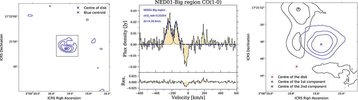
Fig. 9.
Download original image
Residual CO(1–0) emission in NED01 after subtracting the best-fit disk model computed by BBarolo in the Big region. Left: Map of the blueshifted CO(1–0) residual emission integrated in the range −290 ≲ v[km s−1] ≲ − 200. The blue contours are plotted at 3, 6, 9, 15, and 20σ. The black cross indicates the centre of the best-fit molecular disk. The blue cross indicates the peak of the CO(1–0) residual emission. The residual structure can be enclosed within a box of 8.4″ × 8.4″ (∼3 kpc, see black box overlayed on the map). Centre: Spectrum of the CO(1–0) residual emission extracted from an aperture corresponding to the black box shown in the left panel. The two CO(1–0) peaks are fit with double-Gaussian functions whose parameters are reported in Table 4. Right: Map of the two blueshifted spectral components visible in the central panel, plotted with different colours. The first component (blue contours) is the most blueshifted spectral peaks, integrated within v ∈ [ − 400, −200] km s−1; the second component (in black) corresponds to the secondary peak, integrated between v ∈ [ − 200, 0] km s−1. Contours are plotted at 3, 6, 9, 15, and 20σ.
Current usage metrics show cumulative count of Article Views (full-text article views including HTML views, PDF and ePub downloads, according to the available data) and Abstracts Views on Vision4Press platform.
Data correspond to usage on the plateform after 2015. The current usage metrics is available 48-96 hours after online publication and is updated daily on week days.
Initial download of the metrics may take a while.