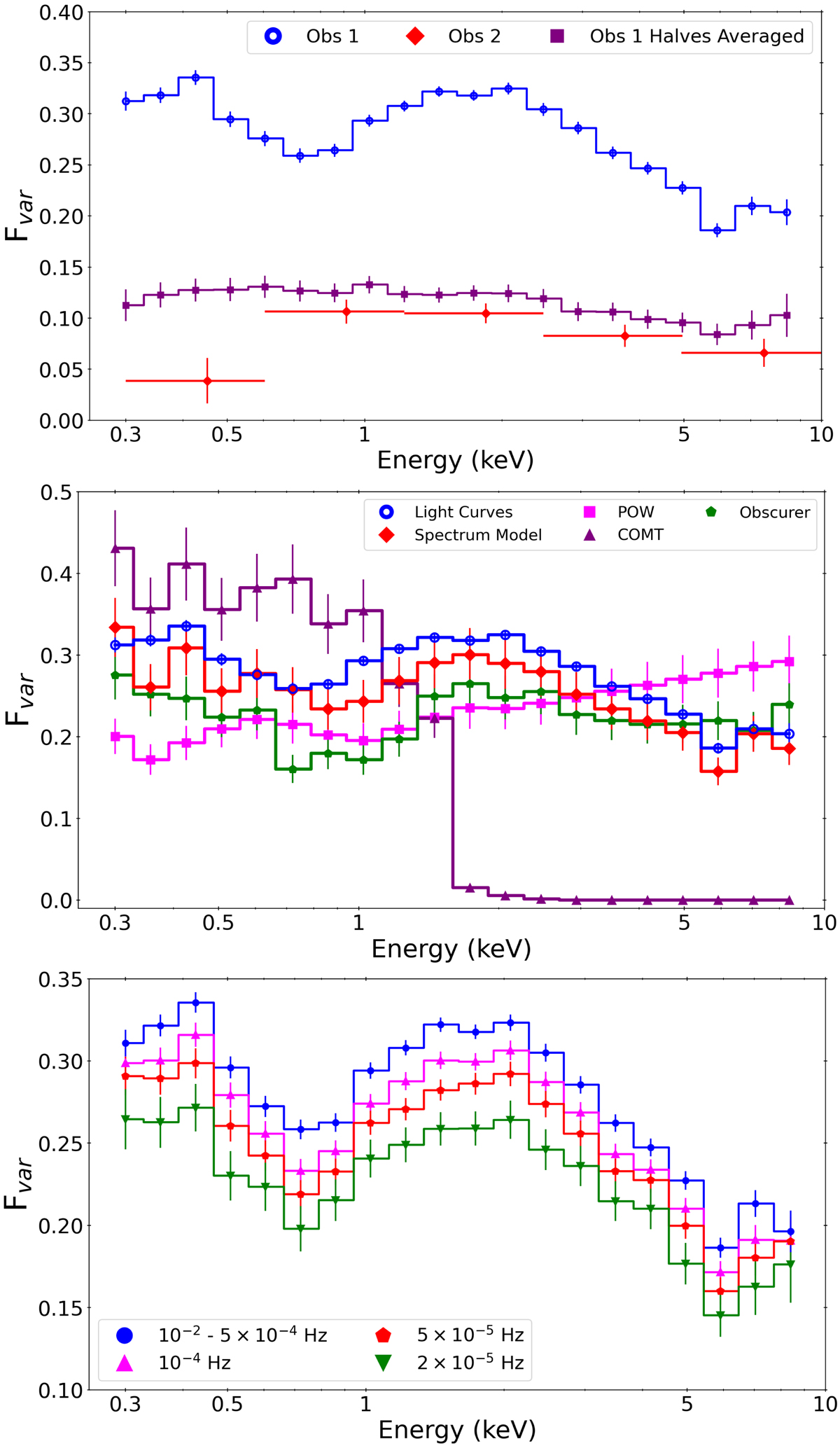
Fractional root mean square (rms) variability amplitude (F_var) spectra as a function of energy. Top panel: Obs 1 (blue circles) and Obs 2 (red diamonds), where the light curves were binned at 1000 s. For Obs 1, the energies are binned logarithmically such that the 20 data points are evenly spaced. For Obs 2, large energy bins are used to remove negative excess variance () values caused by the significant drop in flux compared to Obs 1; the bin sizes are displayed by the x-axis error bars. The purple F_var spectrum shows the results from averaging the two halves of Obs 1. See Sect. 5.4 for details. Middle panel: Fractional rms variability amplitude spectra for the best fit spectral model (red line) and the three main model components: POW (magenta line), COMT (purple line), and the obscurer (PION; green line). The blue line shows the spectrum from the light curves (see top panel). From this plot, it appears that the COMT component drives the fractional rms variability below 1 keV, while the obscurer drives the F_var spectrum between 1 and 5 keV; above 5 keV POW dominates. Bottom panel: Fractional rms variability amplitude spectra comparing different timing bins for the EPIC-PN light curves from Obs 1. The frequencies are 10⁻² – 5 × 10⁻⁴ Hz (Δt = 100, 500, 1000 and 2000 s; blue), 10⁻⁴ Hz (Δt = 10 ks; magenta), 5 × 10⁻⁵ Hz (Δt = 20 ks; red), and 2 × 10⁻⁵ Hz (Δt = 50 ks; green). The shape of each curve stays consistent between frequency bands, suggesting that the model components vary for all light curve timing bins.