| Issue |
A&A
Volume 671, March 2023
|
|
|---|---|---|
| Article Number | A49 | |
| Number of page(s) | 8 | |
| Section | Stellar atmospheres | |
| DOI | https://doi.org/10.1051/0004-6361/202243068 | |
| Published online | 06 March 2023 | |
Mass outflow from the symbiotic binary RS Oph during its 2021 outburst★
1
Institute of Astronomy and NAO, Bulgarian Academy of Sciences,
Tsarigradsko Shausse 72,
1784
Sofia, Bulgaria
e-mail: mtomova@astro.bas.bg
2
Department of Physics and Astronomy, Shumen University Episkop Konstantin Preslavski,
115 Universitetska Str.,
9700
Shumen, Bulgaria
3
Institute of Astronomy of the Russian Academy of Sciences,
48 Pyatnitskaya Str.,
119017
Moscow, Russia
Received:
8
January
2022
Accepted:
13
December
2022
Context. RS Oph is a symbiotic recurrent nova containing a massive white dwarf with heavy mass loss during activity. In August 2021, it underwent its seventh optical eruption since the end of the 19th century.
Aims. The goal of this work is to analyse the structure of the outflows from the outbursting object.
Methods. Based on broad-band U, B, V, RC, and IC photometry and high-resolution Hα spectroscopy obtained at days 11–15 of the outburst, we derived some parameters of the system's components and outflows and their changes during our observation.
Results. The effective temperature of a warm shell (pseudophotosphere) produced by the ejected material and occulting the hot component of the system was Teff = 15 000 ± 1000 K and the electron temperature of the nebula was Te = 17 000 ± 3000 K throughout the observations. The effective radius of the pseudophotosphere was Reff = 13.3 ± 2.0 R⊙ and the emission measure of the nebula EM = (9.50 ± 0.59) × 1061 cm−3 for day 11 and Reff = 10.3 ± 1.6 R⊙ and EM = (5.60 ± 0.35) × 1061 cm−3 for day 15. To provide this emission measure, the bolometric luminosity of the outbursting object must exceed its Eddington limit. The mass-loss rate of the outbursting object through its wind is much greater than through its streams. The total rate (from wind + streams) was less than (4–5) × 10–5 (d/1.6 kpc)3/2 M⊙ yr–1. The streams are not highly collimated. Their mean outflowing velocities are υb = −3680 ± 60 km s–1 for the approaching stream and υr = 3520 ± 50 km s–1 for the receding one if the orbit inclination is 50°.
Key words: binaries: symbiotic / stars: activity / stars: mass-loss / stars: winds, outflows / stars: individual: RS Oph
© The Authors 2023
 Open Access article, published by EDP Sciences, under the terms of the Creative Commons Attribution License (https://creativecommons.org/licenses/by/4.0), which permits unrestricted use, distribution, and reproduction in any medium, provided the original work is properly cited.
This article is published in open access under the Subscribe to Open model. Subscribe to A&A to support open access publication.
1 Introduction
Symbiotic stars are detached binaries consisting of a normal cool giant of spectral type G, K, M, or Mira and a hot compact object accreting mass from the wind of the giant. As a result of the accretion, symbiotic stars evolve through phases of quiescence and activity. The profiles of the spectral lines of some of these binaries have high-velocity satellite components indicating mass loss through bipolar collimated outflows. However, most of these systems show indications of collimated outflows only during active phases, when in addition to the satellite components, their profiles contain wind components; for example P Cyg absorptions and/or broad emissions formed by an optically thin high-velocity wind (e.g. MWC 560, Tomov & Kolev 1997; Hen 3-1341, Tomov et al. 2000; Z And, Tomov et al. 2007; RS Oph, Skopal et al. 2008; and BF Cyg, Skopal et al. 2013). Broad emissions are determined by the kinematics of the emitting gas and in some cases their width is a measure of the speed of a shock wave generated by the ejecta (Sokoloski et al. 2006). The Hα line of the symbiotic stars is emitted in all parts of their circumbinary envelope and its profile contains several components during activity.
The system RS Oph is a prototype of the recurrent symbiotic novae, and consists of an M2 III giant (Zamanov et al. 2018) and a white dwarf with a mass close to the Chandrasekhar limit (Bode 1987, and references therein) with an orbital period of 456d (Fekel et al. 2000; Brandi et al. 2009). Seven optical outbursts of RS Oph with light maxima in 1898, 1933, 1958, 1967, 1985, 2006, and 2021 have been recorded.
A typical feature of the system RS Oph during its previous outbursts is the shape of the remnant from the nova explosion, which is far from spherical and is more close to a bipolar nebula. During the previous 2006 outburst, radio data were obtained with MERLIN, VLA, VLBA, and EVN arrays (O'Brien et al. 2006). The data obtained at days 13÷49 after the beginning of the outburst reveal several components of the radio image that appear at different times. This behaviour is thought to result from an expanding shock wave, which sweeps through the wind of the cool giant creating a high-temperature region. The components of the radio image were modelled with a bipolar shock-heated shell whose axis is perpendicular to the orbital plane. The hypothesis of the outward-moving shock wave was confirmed by the results of X-ray observations (Sokoloski et al. 2006), which allowed the conditions within the ejecta to be diagnosed. The flux in the energy range 2–20 keV was fitted with a single-temperature thermal free-free emission, Fe II emission lines, and absorption by intervening material. During the first three weeks of the outburst, the flux faded strongly, and its high-energy part faded the most, indicating a drop in temperature. The rapid fading of the X-ray flux suggests that the nova explosion deviates from a spherically symmetric blast wave. The system RS Oph was observed in the X-ray domain several years after its 2006 outburst as well. In 2009 and 2011, the Chandra Observatory detected an extended emission consistent with a bipolar flow seen from the system in opening angles of about 70° (Montez et al. 2022). The lengths of both lobes grew and in 2011 the lengths reached 2.0 arcsec projected on the sky. No evidence of cooling of the ejected gas was found and on this basis it was concluded that it had expanded freely, driven by some mechanism of collimation away from the system. It was also concluded that the ejected gas moved into some cavity formed by the 1985 outburst. The circumbinary medium in RS Oph was modelled by Booth et al. (2016). One of the results of this latter study is that the mass transferred to the white dwarf concentrates towards the orbital plane and forms an accretion disc that extends to the boundary of the Roche lobe. The spherical ejecta of the outbursting dwarf interact with the disc and produce a highly bipolar nebular structure with a dense equatorial ring.
At the very beginning of the previous 2006 outburst, the Hα profile of RS Oph comprised three components: a weak narrow central double peak emission, a very intensive triangular broad component with a full width at zero intensity (FWZI) of about 7600 km s−1 emitted in an optically thin stellar wind from the outbursting object, and a blueshifted absorption with a velocity of about 4250 km s−1. After that, the line changed, acquiring a central intensive emission with a triangular shape again and FWZI ~ 3500 km s−1, which was interpreted as a slowly expanding equatorial ring-like structure and satellite emissions on both sides of the central one with velocity position of ~2500 km s−1, indicating bipolar collimated outflow. After the first month of the outburst, the satellite emissions disappeared and a high-velocity wind was observed in the Hα wings only (Skopal et al. 2008). Satellite emission components at the same velocity position in the lines Paβ and Brγ were observed during the first month of this outburst by Banerjee et al. (2009) as well. In addition, satellite emissions of the lines of He I and He II with much lower velocities of about 200 km s−1 were observed by Iijima (2009) and Brandi et al. (2009) in March and April 2006.
The present 2021 outburst of RS Oph began on August 8.93 (Geary 2021) and was observed over the whole electromagnetic domain. High-resolution optical spectroscopy during its first 2–3 days was obtained by Munari & Valisa (2021a), Mikolajewska et al. (2021) and Taguchi et al. (2021). One excellent atlas showing the evolution of the optical spectrum of RS Oph from August 9 to 26 and containing data from every night in this period was presented by Munari & Valisa (2021b). At the beginning of the outburst, the Hα profile comprised an intensive narrow central emission with a sharp absorption on its blue side, an intensive triangular broad component with FWZI ~ 6000 km s−1 produced by the ejecta, and a deep P Cyg absorption at ~3000–4000 km s−1, which disappeared after August 13. The central emission decreased strongly during the observation. In the first two days, the width of the broad emission increased and its FWZI reached about 7000 km s−1, keeping this value until the end of observation. However, the full width at half maximum (FWHM) of the line began to decrease after August 12 and the profile acquired a shape more closely resembling a bell than a triangle. In addition, the Hα line had weak emission bumps on its wings, which could be the signature of a bipolar outflow; these were visible from August 12 to 26.
We observed the Hα line in several nights starting 11 days after the beginning of the outburst. Our main aim is to investigate the structure of the outflowing material from the outbursting object on the basis of the Hα profile. One complementary task is to estimate its mass-loss rate.
2 Observations and data reduction
The region of the Hα line of RS Oph was observed with the Andor Newton CCD camera mounted on the Coude spectrograph of the 2 m Ritchey-Chretien–Coude (RCC) telescope of the National Astronomical Observatory Rozhen, Bulgaria. The observed wavelength window was 225 Å and the spectral resolution was 0.11 Å px−1. Several spectra were taken every night from August 19 to 23. The list of observations is presented in Table 1. Some of these spectra were used in the work of Zamanov et al. (2022). The spectra from each particular night were added together to improve their signal-to-noise ratio (S/N). The data were reduced in the standard way using the IRAF package1.
To build a spectral energy distribution of the system we used average U, B, V, RC, and IC photometric estimates from the light curves of the AAVSO observers taken during our observations. The energy fluxes were calculated using data from Bessell (1979) for a zero-magnitude star. The continuum flux at the position of Hα was obtained using linear interpolation of the RC and IC continuum fluxes. The Hα flux was obtained from the equivalent width and continuum flux at the position of this line. The BVRCIC fluxes were corrected for the strong emission lines of RS Oph by means of low-resolution spectra from the Astronomical Ring for Access to Spectroscopy database2 (ARAS; Teyssier 2019) also taken during our observations. The ARAS spectra are of different S/N. We measured the equivalent widths of eight lines in B band, eight in V band, six in RC band, and 3 in IC band. In addition to these lines, RS Oph has other weak emission lines that are not measurable and whose total contribution is smaller than the uncertainty of the continuum fluxes. We calculated a correction for every night, but as it changed within the limits of our accuracy, we took its arithmetical mean for all spectra. Its mean values are 41.8 ± 2.2%, 25.4 ± 1.8%, 53.4 ± 2.4%, and 15.0 ± 1.7% for the photometric bands B, V, RC, and IC. However, the range of the ARAS spectra does not include the photometric band U and moreover these spectra are too noisy in the region of the Balmer jump. Nevertheless, we used a U flux available for August 23 without these corrections but dered-dened. The U BVRCIC fluxes were obtained with an uncertainty of 4.6% and are listed in Table 1. The continuum and Hα fluxes were dereddened with use of E(B − V) = 0.69 (Zamanov et al. 2018) and the extinction curves of Cardelli et al. (1989).
3 Continuum energy distribution
To examine the outflow structure of the outbursting compact object, we require an estimate of the inner boundary of the outflows. The spectral energy distribution of the system RS Oph shows that the observed photosphere (pseudophotosphere) of the outbursting object at the time of maximal light in 2006 and several days later had an enormous effective radius of 160–200 R⊙ and a low temperature of about 6000–9000 K. After the seventh day of the outburst, the radius decreased to 1–2 R⊙ and the temperature increased to about 110 000 K (Skopal 2015a). This is why it was also necessary to build the energy distribution at the time of our spectral observations in order to determine the effective radius of the pseudophotosphere. We were able to provide ourselves with U BVRCIC photometry only and were not able to find any UV flux at this time. The duration of our observations was five days (Table 1) and the brightness of RS Oph changes slightly over one day. If we build the energy distribution for every day, the distributions will differ slightly but within the limits of our accuracy. This is why we only built the energy distribution for the first and last day of our observations.
To calculate the fluxes of the pseudophotosphere and circumbinary nebula, we need to know the fluxes of the cool giant. Assuming that the giant does not change (Skopal 2015a,b), we subtracted the fluxes of the giant obtained by Skopal (2015a) from the observed fluxes and approximated their residuals separately with a Planck function and nebular continuum determined by recombinations and free-free transitions. The Planck continuum is determined by the effective temperature and radius of the observed photosphere (pseudophotosphere) of the out-bursting object. The nebular continuum is determined by the electron temperature and emission measure of the nebula. We built a number of model continua, varying these four parameters, and estimated their values at which the residual between the model fluxes of the system and the observed ones is minimal. As required by our treatment, we accepted a helium abundance of 0.1 (Vogel & Nüssbaumer 1994) in the nebula. In order to model the nebular continuum, we had to also determine the dominant state of ionisation of helium. The data of Munari & Valisa (2021b) show that the lines of He II are not present in the spectrum of RS Oph during the first 18 days of the outburst. That is why we accepted that the dominant state of ionisation of helium in the nebula of RS Oph is He II and its continuum is produced by H I and He I. We used continuum emission coefficients of hydrogen from the paper of Ferland (1980) and those of helium from the book of Pottasch (1984). We accepted a distance to the system of 1.6 kpc, which is the value used in a very comprehensive analysis of the spectral energy distribution by Skopal (2015a,b). We calculated the parameter χ2 using the chi-square method for every one of our solutions, and for the best ones we obtained χ2 = 0.52 for August 19 and χ2 = 0.70 for August 23. The approximation of the U BVRCIC fluxes of RS Oph showed that, for the period of our observation, the effective temperature of the pseudophotosphere and the electron temperature of the nebula have not changed; the former was Teff = 15 000 ± 1000 K, and the latter Te = 17 000 ± 3000 K. The error of the electron temperature was estimated from a comparison of nebular fluxes with different temperatures. This error was calculated so that the residual of the fluxes with different temperatures is not smaller than the uncertainty of the observed fluxes. The error of the effective temperature of the outbursting object was estimated in the same way. We obtained an effective radius for the pseudophotosphere of Reff = (13.3 ± 2.0) (d/1.6kpc) R⊙ and an emission measure for the nebula of EM = (9.50 ± 0.59) × 1061 (d/1.6 kpc)2 cm−3 for August 19 and Reff = (10.3 ± 1.6) (d/1.6kpc) R⊙ and EM = (5.60 ± 0.35) × 1061 (d/1.6 kpc)2 cm−3 for August 23. The errors of these parameters were obtained from the errors of the temperature and observed fluxes. The energy fluxes of the components of the system (SC) are listed in Table 2 where the total fluxes of the system are compared with the observed fluxes. The continuum energy distribution is shown in Fig. 1.
We obtained the parameters of the pseudophotosphere using only a narrow U BVRCIC range. We tried to approximate the fluxes for August 23 with black-body continua with temperatures of 25 000 K, 50 000 K, and 100 000 K and at the same time each of these three continua was used together with nebular continua with temperatures of 17 000 K, as well as 20 000 K to 40 000 K, in steps of 5000 K (Table 3). Table 3 shows the same product r which persists in the last row of Table 2 for each continuum distribution. The last row of Table 2 is added for comparison. If we approximate the observed flux at the position of the IC band in each of these examples, the model flux exceeds the observed one at the position of the shorter wavelength bands because of an increase in the nebular emission towards the short wavelengths coupled with a much steeper increase in the black-body emission. We should remember that the nebular emission produced by recombinations and free-free transitions increases more steeply than our observed fluxes from IC band towards the shorter wavelength bands at all electron temperatures in the range 10 000–40 000 K. This is why in our case it was possible to approximate the observed fluxes of RS Oph with only a black-body emission with a temperature not higher than about 15 000 K and a nebular emission with a temperature of about 17 000 K. The spectrum of a black-body with such a temperature has a maximal intensity at λλ 1932 Å. Its intensity at the wavelength of the B band is only smaller by a factor of 3.4. In this way, such a black-body emits an appreciable part of its spectrum in the U BVRCIC range, which gives us reason to conclude that the parameters obtained are reliable.
Using the determined quantities, we are able to compare the parameters of the pseudophotosphere and the emission measure of the nebula. The condition for ionisation equilibrium between the number of ionising photons (Lyman photon luminosity) and the rate of recombination in the nebula is
 (1)
(1)
where αB(H,Te) is the recombination coefficient to all but the ground state of hydrogen (Case B). If μ ≧ 1, only radiative ionisation is realised. The equality is fulfilled when all photons are absorbed in the nebula. If μ < 1, both kinds of ionisation are realised, radiative and shock. Their ratio is (1 − μ)/μ, where μ denotes the nebular continuum flux produced by the radiative ionisation and 1 − μ is the nebular continuum flux produced by the shock ionisation. In some cases of distribution of the circumbinary gas, some of the ionising photons can leave the nebula. In these cases, (1 − μ)/μ is a lower limit of the ratio of the continua produced by shock and radiative ionisations. In our calculations, we used αB(H,Te) = 1.67 10−13 cm3 s−1 and the function giving the number of ionising photons for hydrogen G0 = 0.1 from the paper of Nüssbaumer & Vogel (1987). For August 19, we obtained Lph = (2.30 ± 0.93) × 1047 phot s−1 and αB(H,Te)EM = (1.74 ± 0.11) × 1049 s−1 and for August 23 Lph = (1.38 ± 0.57) × 1047 phot s−1 and αB(H,Te)EM = (1.03 ± 0.06) × 1049 s−1. In both cases, Lph ≪ α(H,Te)EM which means that both kinds of ionisation are realised. On the other hand, the X-ray observations show that only small areas in the nebula are heated by shock and have a high temperature of 106 ÷ 107 K and an emission measure of 1058 cm−3 (Sokoloski et al. 2006). We obtained a low effective temperature of 17 000 K and an emission measure of about 1062 cm−3, which exceeds the emission measure of the shock-heated areas by a factor of four orders of magnitude. We therefore prefer the supposition that the circumbinary nebula in RS Oph is mainly radiatively ionised; in other words, the observed rate of recombination can be produced by a hot ionising star with Lph ≧ 1.74 × 1049 phot s−1 and Lph ≧ 1.03 × 1049 phot s−1 in the two cases. The star is occulted by its pseudophotosphere and ionises the nebula up and down, which means that this pseudophotosphere should be disc-shaped. Such a shell can result from interaction of the outflowing material with an accretion disc (see the Sect. 4). This is why for the inner boundary of the outflows (ejecta), we should not accept the radius of the pseudophotosphere (shell) but rather a radius close to that of the white dwarf in the quiescent state of the system. A white dwarf with a mass of 1.2–1.4 M⊙ has a radius of 0.006–0.002 R⊙ (Magano 2017). The effective radius of the underlying (occulted by the shell) outbursting component is not likely to be equal to the radius of the white dwarf because of expansion. Skopal (2015b) came to the conclusion that the temperature of the outbursting object 100 days after the beginning of the 2006 outburst is higher than 100 000 K. We set the temperature and effective radius of the underlying outbursting object in such a way that its Lyman luminosity is equal to or a little greater than the number of recombinations in the nebula for the two dates. If we accept a temperature of 150 000 K and effective radius of 0.9 R⊙ for August 19, the Lyman luminosity will amount to Lph = 2.12 × 1049 ≳ 1.74 × 1049 phot s−1. If we accept the same temperature and an effective radius of 0.7 R⊙ for August 23, the Lyman luminosity will amount to Lph = 1.28 × 1049 ≳ 1.03 × 1049 phot s−1. This is why for the inner boundary of the outflows during our observations, we will take a radius for each date interpolated between 0.9 R⊙ and 0.7 R⊙.
Journal of observations of RS Oph.
Continuum fluxes of the system's components in units of 10−12 erg cm−2 s−1 Å−1.
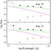 |
Fig. 1 Continuum energy distribution of RS Oph in the UBVRCIC range. The lines designate the black body and nebular continua and the triangles show the fluxes of the giant. The crosses designate the total fluxes and the points show the observed fluxes. |
Product r = (TF−OF)/OF in % for August 23 for a number of continuum distributions obtained with a relevant set of electron temperatures for several effective temperatures.
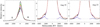 |
Fig. 2 Hα line. Left panel: evolution of Hα line. The spectrum of lowest intensity relates to August 19. Middle and right panels: area of the wings of the line where satellite components are seen. Approximating curves are also shown: blue colour shows line components, and the red colour shows the resulting curve approximating the observed spectrum. |
4 Analysis of the Hα profile and mass-loss rate
At the time of our observations, the central narrow emission was very weak and we considered only the very intensive broad component of Hα. This component had an appreciated asymmetry and very broad low-intensity wings reaching ±3500 km s−1 from the centre of the line (Fig. 2). The width of the wings shows very high ejection velocity and we assume this to be related to nebular material ejected by the outbursting component. As the Hα profile had an appreciable FWHM of 1100–1400 km s−1 in addition, we conclude that the whole line was emitted mainly by the ejecta. In the period of our observations, the relative intensity of Hα increased at decreasing FWHM and a practically constant FWZI of 7000 km s−1 (Fig. 2; and see below). However, Hα had very weak broad bumps on its wings at a velocity position of ±(2300 ÷ 2400) km s−1 as well. The redshifted one is weaker and, for this reason, less visible. The bumps are marked with arrows in the left panel of Fig. 2. The line Hα had similar bumps on its wings during the 2006 eruption as well, which were analysed by Skopal et al. (2008). These authors concluded that these bumps represent satellite line components at the velocity position of about ±2400 km s−1 and are an indication of bipolar collimated outflow. On the other hand, the blueshifted bump seen during our observations was variable and was double peaked on our last spectrum, which means it is an individual component of the line (Fig. 2). This is why we are inclined to suppose that the emission bumps observed by us during the 2021 eruption of this system represent satellite components, and are an indication of bipolar outflow from the outbursting component as well. However, it should be noted that, as is seen in Fig. 2 from the work of Skopal et al. (2008), the satellite components during the 2006 eruption were much more intense relative to the central emission of the line than during the 2021 eruption.
To obtain the parameters of the stellar wind and bipolar outflow, we analysed the Hα profile by means of approximation with different functions: because of its asymmetry, the central emission together with the wings was approximated with a sum of Gaussian and Lorentzian and each bump was approximated with one Gaussian (Fig. 2). For approximation of the bumps, we adopted FWZI = 2 FWHM. The parameters of the central emission and satellite components obtained with this procedure are listed in Tables 4 and 5. The error of the equivalent width of the central emission is determined primarily by the uncertainty in the approximation of the continuum level and is less than 1.5%. The error of the flux, luminosity, and emission measure of the central emission is less than 5%. The bumps are weak broad emission components and it is difficult to determine their extension precisely. The error of their equivalent width results from their approximation and the uncertainty in the approximation of the continuum level and is not more than 26% for all spectra. The errors on their FWHM and velocity position result mainly from the approximation; the former is 3% and the latter is 2%. The error on the energetic flux of the satellite components is 26%.
A number of the analyses presented here show that the ejection of mass during the outburst of RS Oph is not spherical and is closer to bipolar (O'Brien et al. 2006; Booth et al. 2016; Montez et al. 2022). Booth et al. (2016) modelled the circumstellar medium in RS Oph in quiescence and during outburst. These authors obtained a bipolar structure of the wind of the outbursting component resulting from the interaction of a spherical nova outburst with the accretion disc. As is seen from their Fig. 3, the wind propagates in a linear angle of about 120°. For our calculations, we accept a model of a bipolar wind propagating at a linear angle of 120° as well. We calculated the mass-loss rate Ṁ from the Hα flux supposing that the wind has a constant velocity υ and using the nebular approach of Vogel & Nüssbaumer (1994). The energy flux of a bipolar nebula with a solid angle Ω and a radius r at a distance d is
 (2)
(2)
where α is the recombination coefficient at the upper level of Hα transition. The particle density in the wind is
 (3)
(3)
where μ = 1.4 (Nüssbaumer & Vogel 1987) is the parameter determining the mean molecular weight μmH in the wind. For the velocity of the wind, we accepted υ = 3500 ± 250 km s−1 which is equal to the half width at zero intensity (HWZI) of the line throughout our observations. The data in Table 4 show the EM of Hα is 30−50% of the EM based on the nebular continuum for August 19 and 23, which means that a significant part of the nebular emission of the system is produced by the wind. We then assumed that the dominant state of ionisation of helium in the wind is also He II and the electron temperature is 17 000 K. We used a recombination coefficient for a temperature of 17 000 K and a density of 1011 cm−3 (Storey & Hummer 1995), which is very close to the mean density in the wind. For the inner boundary of the wind, we took the radius of the outbursting component calculated at the end of Sect. 3. The outer boundary of integration was determined in the following way. After the beginning of the outburst, the ejected material creates an expanding lobe inside the wind of the giant (Girard & Willson 1987; Nüssbaumer & Walder 1993; Bisikalo et al. 2006). The expansion velocity decreases with time because the expansion is slowed by the wind of the giant, and reaches a final value of
 (4)
(4)
where m = Ṁ/Ṁ0, ω = υ/υ0, and υ0, Ṁ0, υ, and Ṁ are the wind velocities and mass-loss rates of the giant and outbursting component, respectively (Girard & Willson 1987). Using the parameters of the wind from the giant υ0 = 20 km s−1 and Ṁ0 = 5 × 10⁻⁷ M⊙ yr−1 (Booth et al. 2016) and the parameters that we obtained for the outbursting component υ = 3500 km s−1 and Ṁ = 5 × 10⁻⁵ M⊙ yr−1, we derived υshell = 1520 km s−1. For 15 days after the beginning of the outburst, the lobe, which is filled by this newly appearing wind and is expanding with this latter velocity, should reach a size of 13.2 au. However, as our observations were made at a very early stage of the outburst, we suppose that the real expansion velocity is closer to the observed wind velocity than to υshell and therefore we used the observed velocity. For an expansion for 15 days, we obtained a size of the lobe of 30.3 au. This size was used as an outer boundary of the wind. The parameters of the wind are listed in Table 4 for each date of observation. The error of the mass-loss rate is 7%. The change of the mass-loss rate from (5.0 ± 0.4) × 10−5 (d/1.6 kpc)3/2 M⊙ yr−1 to (4.0 ± 0.3) × 10−5 (d/1.6 kpc)3/2 M⊙ yr−1 is greater than this latter error and we conclude that it decreased during our observations. We hypothesise that the rate decreased more quickly but our result is influenced by the increase in the contribution of the other parts of the circumbinary nebula in the central emission of Hα when the system returns to its quiescent state. The decrease in the wind contribution to the central emission is indicated by the diminution of its FWHM. This is why we consider our result as an upper limit of the mass-loss rate. Skopal et al. (2008) obtained a mass-loss rate of the outbursting component of (1–2) × 10−4 (d/1.6 kpc)3/2 M⊙ yr−1 for day 1.38, which is close to the light maximum of the 2006 eruption of RS Oph. The mass-loss rate that we obtain here for days 11–15 of the 2021 eruption is less than (4–5) × 10−5 (d/1.6 kpc)3/2 M⊙ yr−1.
The next task of our investigation is to calculate the mass-loss rate from the bipolar streams of the outbursting component, which are indicated by the satellite components. We used the same nebular approach, supposing that the outflowing material propagates with a constant velocity in two spherical sectors with a small linear angle. The linear angle θ and solid angle Ω of a spherical sector were calculated using the parameters of the satellite components and orbit inclination, adopting the approach of Skopal et al. (2009). We used an orbit inclination of 50° according to Brandi et al. (2009). We also used the same electron temperature and boundaries of integration as for the wind. The parameters of the two streams are listed in Table 5 for each date of observation. The mean velocities of the satellite components of υb = −2360 ± 40 km s−1 for the blueshifted component and υr = 2260 ± 30 km s−1 for the redshifted component are very close to their velocity during the 2006 eruption (Skopal et al. 2008). The linear angle θ shows that the streams are not highly collimated. The error of the mass-loss rate of the compact object through the streams is 26%. The change of the mass-loss rate slightly exceeds its error and we conclude that it did not vary during our observations, having a mean value of Ṁb = (1.1 ± 0.3) × 10−6 (d/1.6 kpc)3/2 M⊙ yr−1 for the approaching stream and Ṁr = (0.6 ± 0.2) × 10−6 (d/1.6 kpc)3/2 M⊙ yr−1 for the receding one. It is seen from Tables 4 and 5 that the mass-loss rate from the streams is a small part of the total mass-loss rate (wind + streams) for the outbursting object.
The density in an outflow with a constant velocity decreases with the radius as r−2 (Eq. (3)). However, we can obtain one tentative estimate of the size of the high-velocity portion of the streams emitting satellite components if we consider them as spherical sectors with a constant density. In this case, we can obtain their volume from their emission measure. The density in the streams is very close to the density in the wind and we assumed the same mean density of 1011 cm−3. The mean emission measure and solid angle of the approaching stream of 2.77 × 1059 cm−3 and 0.4010 sr lead to a radius of the spherical sector of rb = (85 ± 8) (d/1.6 kpc) R⊙ if the error of the emission measure is 26%. The mean emission measure and solid angle of the receding stream of 1.38 × 1059 cm−3 and 0.2584 sr lead to a radius of the spherical sector of rr = (78 ± 7) (d/1.6 kpc) R⊙. These radii are tentative estimates of the size of the streams.
Parameters of the central Hα emission.
Parameters of the satellite components.
5 Discussion
For the first and last day of our observation, August 19 and 23, we find the rate of recombination in the nebula of RS Oph to be much greater than the Lyman luminosity of the ionising star. To balance the rate of recombination, the Lyman luminosity should be Lph ≧ 1.74 × 1049 phot s−1 and Lph ≧ 1.03 × 1049 phot s−1 for these two days. According to Skopal (2015b), the temperature of the outbursting object increases to more than 100 000 K after the light maximum of the 2006 eruption of RS Oph. We accepted a temperature of 150 000 K and radii of 0.9 R⊙ and 0.7 R⊙ for August 19 and 23, and obtained Lyman luminosities of 2.12 × 1049 phot s−1 and 1.28 × 1049 phot s−1, respectively. These temperature and radii give enormous bolometric luminosities of 3.7 × 10⁵ L⊙ and 2.2 × 10⁵ L⊙, which exceed the Eddington luminosity of the hot component in RS Oph by factors of 8 and 5, respectively. From his multi-wavelength modelling of the continuum energy distribution, Skopal (2015a) obtained a temperature of 110 000 K and a radius of 2.1 R⊙ at day 7.3 after the beginning of the 2006 outburst, which lead to an equally enormous bolo-metric luminosity of 5.8 × 10⁵ L⊙, exceeding the Eddington limit by a factor of more than 13. At day 19.5, the bolometric luminosity exceeded the Eddington limit by a factor of more than 4. These data propose a similar behaviour of the outbursting component during the two eruptions. Immediately after the maximal light of both eruptions, the emission measure of the circumbinary nebula was 1062 cm−3 (Skopal 2015a, this paper). One remarkable feature of the RS Oph system is that during the 2021 eruption, about 30%–50% of the nebular emission belongs to the high-velocity wind. The luminosity of the wind in Hα reaches 2900 L⊙ during the 2006 eruption (Skopal et al. 2008) and less than 2700 L⊙ during the 2021 one (result from the present paper).
6 Conclusion
We present results of high-resolution Hα observations and simultaneous U, B, V, RC, and IC photometry from the AAVSO database carried out soon after the light maximum of the 2021 outburst of the symbiotic nova RS Oph. We analysed the continuum energy distribution of the system at the first and last day of our observation, namely August 19 (day 11 of the outburst) and August 23 (day 15). Our results show that the effective temperature of the outbursting component was Teff = 15 000 ± 1000 K and the electron temperature of the nebula Te = 17 000 ± 3000 K for the whole period of observation. The effective radius of the observed photosphere (pseudophotosphere) was Reff = (13.3 ± 2.0) (d/1.6 kpc) R⊙ and the emission measure of the nebula EM = (9.50 ± 0.59) × 1061 (d/1.6 kpc)2 cm−3 for August 19 and Reff = (10.3 ± 1.6) (d/1.6 kpc) R⊙ and EM = (5.60 ± 0.35) × 1061 (d/1.6 kpc)2 cm−3 for August 23. These data show that the Lyman photon luminosity of this pseudophotosphere is insufficient to balance the rate of recombination in the nebula, which, in turn, means we observed a disc-shaped warm shell occulting the central hot object. This shell could appear as the result of a collision between the ejected material and an accretion disc. The hot object ionises the nebula up and down and produces the observed emission measure. To provide this emission measure, its bolometric luminosity should exceed several times its Eddington limit.
We analysed the Hα profile with the aim being to study the outflow structure. Throughout the period of observation, the Hα appeared as a very intense, broad emission line with an FWHM of 1100–1400 km s−1 and FWZI of 7000 km s−1, possessing weak broad bumps at its wings with mean velocities of υb = −2360 ± 40 km s−1 and υr = 2260 ± 30 km s−1. We conclude that most of the central emission is produced by the ejected material from the outbursting component (stellar wind) and the bumps are satellite components indicating bipolar outflow. We also find that about 30–50% of the nebular emission of the system belongs to the wind, the Hα luminosity of which was less than 2700 L⊙. We determined the mass-loss rate of the outbursting component from those of the wind and the streams. The mass-loss rate from the streams is a small part of the total rate, whose upper limit decreased from (5.2 ± 0.4) × 10−5 (d/1.6 kpc)3/2 M⊙ yr−1 to (4.1 ± 0.3) × 10−5 (d/1.6 kpc)3/2 M⊙ yr−1 during our observations. Our results suggest the streams were not highly collimated, and we obtained one tentative estimate of their size, which amounts to about 80(d/1.6 kpc) R⊙.
Acknowledgements
The authors are grateful to an anonymous referee for his critical remarks that improved the manuscript. We are grateful to Pierre Dubreuil (P.D.L.), Joan Guarro (J.G.F.), Keith Shank (K.S.H.) and Francois Teyssier (F.T.E.) for their spectroscopic observations as well. We acknowledge with thanks the variable star observations from the AAVSO International Database contributed by observers worldwide and used in this research. The authors gratefully acknowledge observing grant support from the Institute of Astronomy and National Astronomical Observatory, Bulgarian Academy of Sciences. We thank Mr. J. Neve for his work on the language editing of the paper. MTT thanks her sons Alexander and Todor for all their support. MTT is grateful to Alexander Tomov for his efforts and help in preparing the text for publication as well. This work was supported by Bulgarian National Science Fund of the Ministry of Education and Science under grants KP-06-Russia/2-2020 and DN 18-13/2017. D.M. acknowledges partial support by Shumen University Science Fund. P.V.K. was supported by RFBR grant 20-52-18015.
References
- Banerjee, D.P.K., Das, R.K., & Ashok, N.M. 2009, MNRAS, 399, 357 [CrossRef] [Google Scholar]
- Bessell, M.S. 1979, PASP, 91, 589 [CrossRef] [Google Scholar]
- Bisikalo, D.V., Boyarchuk, A.A., Kilpio, E. Yu., Tomov, N.A., & Tomova, M.T. 2006, ARep, 50, 772 [NASA ADS] [Google Scholar]
- Bode, M. 1987, RS Oph (1985) and the Recurrent Nova Phenomenon (VNU Science Press), 241 [Google Scholar]
- Booth, R.A., Mohamed, S., & Podsiadlowski, Ph. 2016, MNRAS, 457, 822 [NASA ADS] [CrossRef] [Google Scholar]
- Brandi, E., Quiroga, C., Mikolajewska, J., Ferrer, O.E., & Garcia, L.G. 2009, A&A, 497, 815 [NASA ADS] [CrossRef] [EDP Sciences] [Google Scholar]
- Cardelli, J.A., Clayton, G.C., & Mathis, J.S. 1989, ApJ, 345, 245 [CrossRef] [Google Scholar]
- Fekel, F.C., Joyce, R.R., Hinkle, K.H., & Skrutskie, M. 2000, AJ, 119, 1375 [NASA ADS] [CrossRef] [Google Scholar]
- Ferland, G.J. 1980, PASP, 92, 596 [CrossRef] [Google Scholar]
- Geary, K. 2021, AAVSO Alert Notice 752 (20210809) [Google Scholar]
- Girard, T., & Willson, L.A. 1987, A&A, 183, 247 [NASA ADS] [Google Scholar]
- Iijima, T. 2009, A&A, 505, 287 [NASA ADS] [CrossRef] [EDP Sciences] [Google Scholar]
- Magano, D.M.N., Vilas Boas, J.M.A., & Martins, C.J.A.P. 2017, Phys. Rev. D, 96, 083012 [NASA ADS] [CrossRef] [Google Scholar]
- Mikolajewska, J., Aydi, E., Buckley, D., Galan, C., & Orio, M. 2021, ATel, 14852 [Google Scholar]
- Montez, R., Luna, G.J.M., Mukai, K., Sokoloski, J.L., & Kastner, J.H. 2022, ApJ, 926, 100 [NASA ADS] [CrossRef] [Google Scholar]
- Munari, U., & Valisa, P. 2021a, ATel, 14840 [Google Scholar]
- Munari, U., & Valisa, P. 2021b, [arXiv:2109.01101] [Google Scholar]
- Nüssbaumer, H., & Vogel, M. 1987, A&A, 182, 51 [Google Scholar]
- Nüssbaumer, H., & Walder, R. 1993, A&A, 278, 209 [Google Scholar]
- O’Brien, T.J., Bode, M.F., Porcas, R.W., et al. 2006, Nature, 442, 279 [CrossRef] [Google Scholar]
- Pottasch, S.R. 1984, Planetary nebulae (Reidel, Dordrecht), 93 [Google Scholar]
- Skopal, A. 2015a, New Astron., 36, 128 [NASA ADS] [CrossRef] [Google Scholar]
- Skopal, A. 2015b, New Astron., 36, 139 [NASA ADS] [CrossRef] [Google Scholar]
- Skopal, A., Pribulla, T., Buil, Ch., Vittone, A., & Errico, L. 2008, in ASP Conf. Ser. 401, RS Ophiuchi 2006 and Recurrent Nova Phenomenon, eds. A. Evans, M.F. Bode, T.J. O’Brien, & M.J. Darnley, 227 [Google Scholar]
- Skopal, A., Pribulla, T., Budaj, J., et al. 2009, ApJ, 690, 1222 [NASA ADS] [CrossRef] [Google Scholar]
- Skopal, A., Tomov, N.A., Tomova, M.T. 2013, A&A, 551, A10 [NASA ADS] [CrossRef] [EDP Sciences] [Google Scholar]
- Sokoloski, J.L., Luna, G.J.M., Mukai, K., & Kenyon, S.J. 2006, Nature, 442, 276 [CrossRef] [Google Scholar]
- Storey, P.J., & Hummer, D.G., 1995, MNRAS, 272, 41 [NASA ADS] [CrossRef] [Google Scholar]
- Taguchi, K., Maehara, H., Isogai, K., Tampo, Y., & Ito, J. 2021, ATel, 14858 [Google Scholar]
- Teyssier, F. 2019, Contrib. Astron. Obs. Skalnate Pleso, 49, 217 [NASA ADS] [Google Scholar]
- Tomov, T., & Kolev, D. 1997, A&AS, 122, 43 [NASA ADS] [CrossRef] [EDP Sciences] [Google Scholar]
- Tomov, T., Munari, U., & Marrese, P. 2000, A&A, 354, L25 [NASA ADS] [Google Scholar]
- Tomov, N.A., Tomova, M.T., & Bisikalo, D.V. 2007, MNRAS, 376, L16 [NASA ADS] [CrossRef] [Google Scholar]
- Vogel, M., & Nussbaumer, H. 1994, A&A, 284, 145 [NASA ADS] [Google Scholar]
- Zamanov, R., Boeva, S., Latev, G., et al. 2018, MNRAS, 480, 1363 [NASA ADS] [CrossRef] [Google Scholar]
- Zamanov, R.K., Stoyanov, K.A., Nikolov, Y.M., et al. 2022, BlgAJ, 37, 24 [NASA ADS] [Google Scholar]
All Tables
Product r = (TF−OF)/OF in % for August 23 for a number of continuum distributions obtained with a relevant set of electron temperatures for several effective temperatures.
All Figures
|
Fig. 1 Continuum energy distribution of RS Oph in the UBVRCIC range. The lines designate the black body and nebular continua and the triangles show the fluxes of the giant. The crosses designate the total fluxes and the points show the observed fluxes. |
| In the text | |
|
Fig. 2 Hα line. Left panel: evolution of Hα line. The spectrum of lowest intensity relates to August 19. Middle and right panels: area of the wings of the line where satellite components are seen. Approximating curves are also shown: blue colour shows line components, and the red colour shows the resulting curve approximating the observed spectrum. |
| In the text | |
Current usage metrics show cumulative count of Article Views (full-text article views including HTML views, PDF and ePub downloads, according to the available data) and Abstracts Views on Vision4Press platform.
Data correspond to usage on the plateform after 2015. The current usage metrics is available 48-96 hours after online publication and is updated daily on week days.
Initial download of the metrics may take a while.