| Issue |
A&A
Volume 666, October 2022
|
|
|---|---|---|
| Article Number | L13 | |
| Number of page(s) | 5 | |
| Section | Letters to the Editor | |
| DOI | https://doi.org/10.1051/0004-6361/202244810 | |
| Published online | 18 October 2022 | |
Letter to the Editor
Analysing the structure of the bulge with Mira variables
1
Instituto de Astrofísica de Canarias, 38205 La Laguna, Tenerife, Spain
e-mail: This email address is being protected from spambots. You need JavaScript enabled to view it.
2
Departamento de Astrofísica, Universidad de La Laguna, 38206 La Laguna, Tenerife, Spain
Received:
25
August
2022
Accepted:
23
September
2022
Abstract
Context. The Galactic bulge at latitude 4 < |b|(deg) < 10 was claimed to show an X-shape, which means that stellar density distributions along the line of sight have a double peak. However, this double peak is only observed with the red-clump population, and doubt has been cast on its use as a perfect standard candle. As such, a boxy bulge without an X-shape is not discarded.
Aims. We aim to constrain the shape of the bulge making use of a different population: Mira variables from the new Optical Gravitational Lensing Experiment data release, OGLE-IV, with an average age of 9 Gyr.
Methods. We analysed an area of the bulge far from the plane, where we fitted the density of the Miras with boxy bulge and X-shaped bulge models and calculated the probability of each model.
Results. We find that the probability of a boxy bulge fitting the data is p = 0.19, whereas the probability for the X-shaped bulge is only p = 2.85 × 10⁻⁶ (equivalent to a tension of the model with the data of a 4.7σ level). Therefore, the boxy bulge model seems to be more appropriate for describing the Galactic bulge, although we cannot exclude any model with complete certainty.
Key words: Galaxy: bulge
© Ž. Chrobáková et al. 2022
 Open Access article, published by EDP Sciences, under the terms of the Creative Commons Attribution License (https://creativecommons.org/licenses/by/4.0), which permits unrestricted use, distribution, and reproduction in any medium, provided the original work is properly cited.
This article is published in open access under the Subscribe-to-Open model. This email address is being protected from spambots. You need JavaScript enabled to view it. to support open access publication.
1. Introduction
The Galactic bulge morphology is an intensely discussed topic. The first near-infrared surveys discovered it to be non-axisymmetric (Weiland et al. 1994; Lopez-Corredoira et al. 1997), but its shape has been debated. Weiland et al. (1994) showed the bulge to have a peanut shape using the Cosmic Background Explorer survey. This peanut shape was later interpreted as the imprint of a boxy bulge (Kent et al. 1991; Dwek et al. 1995; López-Corredoira et al. 2005) due to a composite effect expected to appear considering the stable orbits of several families of periodic orbits (e.g., Patsis et al. 2003).
More recently, the bulge has been reported to have an X-shape, based on an analysis involving red-clump stars (e.g., McWilliam & Zoccali 2010; Wegg & Gerhard 2013; Nataf et al. 2015). These studies find a double peak in the star counts along the line of sight, which leads to an X-shape in the density. However, López-Corredoira (2016) and López-Corredoira et al. (2019) argue that the apparent X-shape could be an artefact and that the red-clump stars do not have a unique narrow peak in their luminosity function. Further doubt was cast by Lee et al. (2015), who attribute the double peak in bulge density to an effect of multiple populations being present in the bulge, although Gonzalez et al. (2015) refute this explanation. The X-shaped bulge was also observed using infrared images of the Milky Way, for example by Ness & Lang (2016). However, these images are dependent on the image processing with the subtraction of some particular disk model or there may be artefacts from subtracting the bulge as an ellipsoid instead of as a boxy bulge (Han & Lee 2018).
In populations other than red-clump populations, the X-shaped bulge is not observed. For instance, very old RR Lyrae stars (Dékány et al. 2013; Pietrukowicz et al. 2015), young populations (≲5 Gyr) such as F0-F5V stars (López-Corredoira 2016), and Mira variables of all ages (López-Corredoira 2017) do not manifest an X-shaped bulge. Vásquez et al. (2013), Ness et al. (2014), and Rojas-Arriagada et al. (2014) presented evidence that the X-shape bulge of the Milky Way is only traced by the metal-rich bulge stars. Recently, Semczuk et al. (2022) analysed the morphology of the bulge with Miras of various ages and found an age-morphology dependence consistent with a boxy or peanut bulge.
Mira variables are pulsating stars, with periods ranging from about 80 to over 1000 days. They are cool giant stars near the tip of the asymptotic giant branch with a high brightness and a well-defined period-luminosity relation, which makes them excellent distance indicators and a useful population for studying Galactic structure (Iwanek et al. 2022). In this Letter we repeat the analysis by López-Corredoira (2017) for the density of the bulge with Mira variables, but with a much larger coverage and number of stars provided by the recent data release of the Optical Gravitational Lensing Experiment survey (OGLE-IV).
The Letter is structured as follows. In Sect. 2 we describe the data selection. In Sect. 3 we derive the density distribution and fit it with models of boxy and X-shaped bulges. In Sect. 4 we conclude.
2. Data
We used OGLE-IV data of Mira variables (Iwanek et al. 2022), carried out with the 1.3 m Warsaw Telescope at the Las Campanas Observatory in Chile. The catalogue covers the whole Galactic bulge area with 40 356 objects, most of them near the plane, and contains an additional 25 625 stars in the Galactic disk, observed in the Johnson V-band (mean wavelength of 0.55 μm) and Cousins I-band (mean wavelength of 0.81 μm) filters.
We analysed the bulge using stars far from the plane (700 pc ≤ |Z|< 1500 pc) in order to avoid the problems of incompleteness due to extinction, and also because the X-shape features are only notable within this range of Z. The completeness is estimated to be 96% (Iwanek et al. 2022); ∼4% of Miras are not classified as such due to the small number of epochs.
3. Analysis
We followed the analysis of López-Corredoira (2017), who carried out an analysis to determine the distances of Mira variables with logP(days) < 2.6 within 58 deg2 in the off-plane bulge. The distances can be calculated using the period-luminosity relationship (Whitelock et al. 2008; Catchpole et al. 2016)
 (1)
(1)
![Mathematical equation: $$ \begin{aligned} \lambda&= \mathrm log_{10} [P(\mathrm{days} )]-2.38 \end{aligned} $$](/articles/aa/full_html/2022/10/aa44810-22/aa44810-22-eq2.gif) (2)
(2)
and the K-band extinction AK = 0.11AV. We determined the extinction AV using the Schlegel et al. (1998) maps. Then, we calculated the apparent magnitude as
 (3)
(3)
where mI is the apparent magnitude in the I filter and (I − K) was determined by López-Corredoira (2017) as (I − K)=3.96 + 3.69λ + 10.33λ2 + 10.98λ3 by calibrating Two Micron All Sky Survey and OGLE data. Finally, for the distance we can use the expression
![Mathematical equation: $$ \begin{aligned} r(m_K)=10^{[m_K-M_K+5]/5}, \end{aligned} $$](/articles/aa/full_html/2022/10/aa44810-22/aa44810-22-eq4.gif) (4)
(4)
where mK is the extinction-corrected K-band magnitude.
The average age of these Mira variables is 9 Gyr, approximately the age of the red-clump samples. The error in the absolute magnitude determination is less than 0.1 mag, which can be neglected. We repeated the analysis for a much wider coverage, the whole bulge off-plane area of ≈250 deg2. As a result we obtained not only the distribution along a few lines of sight, but also a complete 3D distribution of the stars in the whole off-plane bulge. We assumed a galactocentric distance of 8.2 kpc and a position of the Sun over the plane of +17 pc (Karim & Mamajek 2017). We selected only the stars within |X|≤2750 pc, |Y|≤2750 pc, and 700 pc ≤ |Z|< 1500 pc for a total of 2078 stars, which we divided into bins with sizes ΔX = 500 pc, ΔY = 500 pc, and ΔZ = 200 pc. The density maps are plotted in Fig. 1.
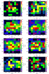 |
Fig. 1. Density, ρ, of Mira variable stars as a function of galactocentric coordinates (the X axis is in the Sun-Galactic centre direction such that X⊙ = +8.2 kpc) in the ranges |X|≤2750 pc, |Y|≤2750 pc, and 700 pc < |Z|< 1500 pc. Bin sizes are 500 × 500 × 200 pc, which implies a Poissonian error of the density in each bin equal to |

For logP(days) < 2.6 Mira variables, the absolute magnitude,  (averaged over the whole period), is lower than −2.6, so for a maximum heliocentric distance of 12 kpc the apparent magnitude,
  , is lower than 12.8 + AI, where AI is the extinction along the line of sight. The maximum amplitude of the variation within the period for these Mira stars in bulge fields is lower than ≈3 magnitudes (Fig. 8, Iwanek et al. 2022). The limiting magnitude is mI, max = 19.0 for |b|> 5° (Udalski et al. 2015), although for very crowded fields at lower latitudes it can be lower (for instance, a value of mI, max = 18.5 at ℓ = 1°, b = −2° was estimated by Udalski et al. 2015). This means that the Mira variables are always below the limiting magnitude, provided that AI < 3 mag. In our range of Galactic latitudes, b, this is the case (Sumi et al. 2003; López-Corredoira 2017). We note, however, that if we wanted to explore lower b regions (lower |Z|), we would lose an important fraction of stars, especially at larger distances.
3.1. Fits of the density.
To fit the data, we used the boxy bulge model from López-Corredoira et al. (2005) and the X-shaped bulge model from Wegg & Gerhard (2013) following the parametrization given by López-Corredoira (2017):
 (5)
(5)
![Mathematical equation: $$ \begin{aligned} \rho _{\text{ X-shape}}(x,y,z)&=\rho _0 \ \mathrm{exp} \left(-\frac{s_1}{700\,\mathrm{pc} }\right)\mathrm{exp} \left(-\frac{|z |}{322\,\mathrm{pc} }\right) \nonumber \\&\quad \times \left[1+3\ \mathrm{exp} \left(-\left(\frac{s_2}{1000\,\mathrm{pc} }\right)^2\right) \right. \nonumber \\&\quad + \left. \ \mathrm{exp} \left(-\left(\frac{s_3}{1000\,\mathrm{pc} }\right)^2\right)\right], \\ s_1&= \mathrm{Max} \left[2100\,\mathrm{pc} , \sqrt{x^2+\left(\frac{y}{0.7}\right)^2} \right], \nonumber \\ s_2&= \sqrt{(x-1.5z)^2+y^2}, \nonumber \\ s_2&= \sqrt{(x+1.5z)^2+y^2}. \nonumber \end{aligned} $$](/articles/aa/full_html/2022/10/aa44810-22/aa44810-22-eq9.gif) (6)
(6)
In Fig. 2 we plot densities of both models compared with the data. We fitted the density maps with only one free parameter, the amplitude ρ0, using the usual least-squares fitting:
 (7)
(7)
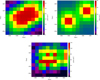 |
Fig. 2. Models of the density averaged for all bins of Z that we use compared with the data. (a): Density of the box bulge. (b): Density of the X-shaped bulge. (c): Data. |
We did not vary the rest of the free parameters, as this sample is not appropriate for fine-tuning the parameters of the models. Fitting the data with the least-squares method and minimizing reduced  leads to a minimal
  for the boxy bulge model and
  for the X-shaped bulge. Since our sample has 967 degrees of freedom, we used the χ2 to calculate the probability, which in the case of a boxy bulge is p = 0.19, whereas in the case of an X-shaped bulge we obtain p = 2.85 × 10⁻⁶. Thus, the boxy bulge fits the density distribution significantly better. For illustration, in Fig. 3 we plot residuals of the fits averaged for every Z, calculated as
 (8)
(8)
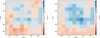 |
Fig. 3. Residuals of least-squares fitting of density averaged for all bins of Z that we use. Left: residuals of the boxy bulge. Right: residuals of the X-shaped bulge. |
where σ stands for the error of data.
We also experimented with changing the fixed parameters of the models to free parameters to explore if this improves the fits. In both cases, the free parameters are almost identical to the fixed values and the  of the fits improved only negligibly. Therefore, we kept the parameters constant and kept only the amplitude as a free parameter.
As the pulsation period is related to the age of the star with the following relationship (López-Corredoira 2017),
 (9)
(9)
with λ defined by Eq. (2), we were able to divide the stars into three groups based on age: logP < 2.38, 2.38 < logP < 2.53, and 2.53 < logP < 2.6, which approximately correspond to ages ≳11.6 Gyr, 6.4–11.6 Gyr, and ≲6.4 Gyr. We fitted each of the populations separately, but in each case χr is significantly lower than 1, and therefore we cannot exclude any model. We conclude that we do not have enough stars of each age to be able to be make separate fits.
In order to improve the fits, we also considered a modification of Eq. (7) for bins with zero density, where we use
 (10)
(10)
where μ is the theoretical expected number of stars per bin. This expression is derived by using  , where fi is the number of sigmas of deviation of an observed point with respect to the theoretical prediction, and calibrating the relationship of fi with a distribution of probabilities, Pi, in a Gaussian distribution, which gives
  . Hence, for a Poissonian distribution in pixels where zero stars are detected and the probability is Pi = exp(−μ), we get the above expression. This modification leads to a small improvement in the fits for the whole dataset, where we obtain minimal
  for the boxy bulge model and
  for the X-shaped bulge. However, for the individual datasets separated by age, we do not see significant improvement: all values of
  are well below 1. Therefore, we consider this modification in the calculation to be
  negligible.
4. Conclusion
We used the recent OGLE data of Mira variables to analyse the shape of the bulge. We derived density maps of the bulge in an area far from the plane (700 pc ≤ |Z|< 1500 pc), which we fitted with density models of a boxy bulge and an X-shaped bulge. Based on least-squares fitting, we calculated the probability of a boxy bulge matching the data to be p = 0.19, whereas the probability of an X-shaped bulge is p = 2.85 × 10⁻⁶ (equivalent to a 4.7σ event). Therefore, the boxy model is more fitting for the shape of the bulge, although we cannot completely exclude any model based on this result. We also separated the stars based on age and tried to analyse each population separately, but we lack a sufficient number of stars to be able to make separate fits. Improving this result only with Mira variables is not possible, since the whole bulge was already covered. However, complementing this dataset with other stellar populations may constrain the possibilities for the morphology of the bulge even more.
Acknowledgments
The authors were supported by the grant PGC-2018-102249-B-100 of the Spanish Ministry of Economy and Competitiveness (MINECO).
References
- Catchpole, R. M., Whitelock, P. A., Feast, M. W., et al. 2016, MNRAS, 455, 2216 [NASA ADS] [CrossRef] [Google Scholar]
- Dékány, I., Minniti, D., Catelan, M., et al. 2013, ApJ, 776, L19 [Google Scholar]
- Dwek, E., Arendt, R. G., Hauser, M. G., et al. 1995, ApJ, 445, 716 [CrossRef] [Google Scholar]
- Gonzalez, O. A., Zoccali, M., Debattista, V. P., et al. 2015, A&A, 583, L5 [NASA ADS] [CrossRef] [EDP Sciences] [Google Scholar]
- Han, D., & Lee, Y. W. 2018, in Rediscovering Our Galaxy, eds. C. Chiappini, I. Minchev, E. Starkenburg, & M. Valentini, 334, 263 [NASA ADS] [Google Scholar]
- Iwanek, P., Soszyński, I., Kozłowski, S., et al. 2022, ApJS, 260, 46 [NASA ADS] [CrossRef] [Google Scholar]
- Karim, T., & Mamajek, E. E. 2017, MNRAS, 465, 472 [NASA ADS] [CrossRef] [Google Scholar]
- Kent, S. M., Dame, T. M., & Fazio, G. 1991, ApJ, 378, 131 [NASA ADS] [CrossRef] [Google Scholar]
- Lee, Y.-W., Joo, S.-J., & Chung, C. 2015, MNRAS, 453, 3906 [Google Scholar]
- López-Corredoira, M. 2016, A&A, 593, A66 [NASA ADS] [CrossRef] [EDP Sciences] [Google Scholar]
- López-Corredoira, M. 2017, ApJ, 836, 218 [CrossRef] [Google Scholar]
- Lopez-Corredoira, M., Garzon, F., Hammersley, P., Mahoney, T., & Calbet, X. 1997, MNRAS, 292, L15 [NASA ADS] [Google Scholar]
- López-Corredoira, M., Cabrera-Lavers, A., & Gerhard, O. E. 2005, A&A, 439, 107 [NASA ADS] [CrossRef] [EDP Sciences] [Google Scholar]
- López-Corredoira, M., Lee, Y. W., Garzón, F., & Lim, D. 2019, A&A, 627, A3 [NASA ADS] [CrossRef] [EDP Sciences] [Google Scholar]
- McWilliam, A., & Zoccali, M. 2010, ApJ, 724, 1491 [NASA ADS] [CrossRef] [Google Scholar]
- Nataf, D. M., Udalski, A., Skowron, J., et al. 2015, MNRAS, 447, 1535 [NASA ADS] [CrossRef] [Google Scholar]
- Ness, M., & Lang, D. 2016, AJ, 152, 14 [NASA ADS] [CrossRef] [Google Scholar]
- Ness, M., Debattista, V. P., Bensby, T., et al. 2014, ApJ, 787, L19 [NASA ADS] [CrossRef] [Google Scholar]
- Patsis, P. A., Skokos, C., & Athanassoula, E. 2003, MNRAS, 342, 69 [NASA ADS] [CrossRef] [Google Scholar]
- Pietrukowicz, P., Kozłowski, S., Skowron, J., et al. 2015, ApJ, 811, 113 [Google Scholar]
- Rojas-Arriagada, A., Recio-Blanco, A., Hill, V., et al. 2014, A&A, 569, A103 [NASA ADS] [CrossRef] [EDP Sciences] [Google Scholar]
- Schlegel, D. J., Finkbeiner, D. P., & Davis, M. 1998, ApJ, 500, 525 [Google Scholar]
- Semczuk, M., Dehnen, W., Schoenrich, R., & Athanassoula, E. 2022, MNRAS, submitted [arXiv:2206.04535] [Google Scholar]
- Sumi, T., Abe, F., Bond, I. A., et al. 2003, ApJ, 591, 204 [NASA ADS] [CrossRef] [Google Scholar]
- Udalski, A., Szymański, M. K., & Szymański, G. 2015, Acta Astron., 65, 1 [NASA ADS] [Google Scholar]
- Vásquez, S., Zoccali, M., Hill, V., et al. 2013, A&A, 555, A91 [NASA ADS] [CrossRef] [EDP Sciences] [Google Scholar]
- Wegg, C., & Gerhard, O. 2013, MNRAS, 435, 1874 [Google Scholar]
- Weiland, J. L., Arendt, R. G., Berriman, G. B., et al. 1994, ApJ, 425, L81 [NASA ADS] [CrossRef] [Google Scholar]
- Whitelock, P. A., Feast, M. W., & Van Leeuwen, F. 2008, MNRAS, 386, 313 [CrossRef] [Google Scholar]
All Figures
|
Fig. 1. Density, ρ, of Mira variable stars as a function of galactocentric coordinates (the X axis is in the Sun-Galactic centre direction such that X⊙ = +8.2 kpc) in the ranges |X|≤2750 pc, |Y|≤2750 pc, and 700 pc < |Z|< 1500 pc. Bin sizes are 500 × 500 × 200 pc, which implies a Poissonian error of the density in each bin equal to |
| In the text | |
|
Fig. 2. Models of the density averaged for all bins of Z that we use compared with the data. (a): Density of the box bulge. (b): Density of the X-shaped bulge. (c): Data. |
| In the text | |
|
Fig. 3. Residuals of least-squares fitting of density averaged for all bins of Z that we use. Left: residuals of the boxy bulge. Right: residuals of the X-shaped bulge. |
| In the text | |
Current usage metrics show cumulative count of Article Views (full-text article views including HTML views, PDF and ePub downloads, according to the available data) and Abstracts Views on Vision4Press platform.
Data correspond to usage on the plateform after 2015. The current usage metrics is available 48-96 hours after online publication and is updated daily on week days.
Initial download of the metrics may take a while.