| Issue |
A&A
Volume 666, October 2022
|
|
|---|---|---|
| Article Number | A71 | |
| Number of page(s) | 7 | |
| Section | Extragalactic astronomy | |
| DOI | https://doi.org/10.1051/0004-6361/202243873 | |
| Published online | 10 October 2022 | |
AGN jets do not prevent the suppression of conduction by the heat buoyancy instability in simulated galaxy clusters
1
Institut d’Astrophysique de Paris, CNRS, Sorbonne Université, UMR7095, 98bis bd Arago, 75014 Paris, France
e-mail: This email address is being protected from spambots. You need JavaScript enabled to view it.
2
Institute of Astronomy and Kavli Institute for Cosmology, University of Cambridge, Madingley Road, Cambridge CB3 0HA, UK
3
AIM, CEA, CNRS, Université Paris-Saclay, Université Paris-Diderot, Sorbonne Paris-Cité, 91191 Gif-sur-Yvette, France
4
SOFIA Science Center, USRA, NASA Ames Research Center, M.S. N232-12, Moffett Field, CA 94035, USA
5
Department of Physics and Astronomy, University of Kentucky, 505 Rose Street, Lexington, KY 40506, USA
Received:
26
April
2022
Accepted:
22
July
2022
Abstract
Centres of galaxy clusters must be efficiently reheated to avoid a cooling catastrophe. One potential reheating mechanism is anisotropic thermal conduction, which could transport thermal energy from intermediate radii to the cluster centre. However, if fields are not re-randomised, anisotropic thermal conduction drives the heat buoyancy instability (HBI) which re-orients magnetic field lines and shuts off radial heat fluxes. We revisit the efficiency of thermal conduction under the influence of spin-driven active galactic nuclei (AGN) jets in idealised magneto-hydrodynamical simulations with anisotropic thermal conduction. Despite the black hole spin’s ability to regularly re-orientate the jet so that the jet-induced turbulence is driven in a quasi-isotropic fashion, the HBI remains efficient outside the central 50 kpc of the cluster, where the reservoir of heat is the largest. As a result, conduction plays no significant role in regulating the cooling of the intracluster medium if central AGN are the sole source of turbulence. Whistler-wave-driven saturation of thermal conduction reduces the magnitude of the HBI, but does not prevent it.
Key words: galaxies: clusters: intracluster medium / methods: numerical / galaxies: magnetic fields / instabilities / galaxies: jets
© R. S. Beckmann et al. 2022
 Open Access article, published by EDP Sciences, under the terms of the Creative Commons Attribution License (https://creativecommons.org/licenses/by/4.0), which permits unrestricted use, distribution, and reproduction in any medium, provided the original work is properly cited.
This article is published in open access under the Subscribe-to-Open model. This email address is being protected from spambots. You need JavaScript enabled to view it. to support open access publication.
1. Introduction
The hot intracluster medium (ICM) is a substantial thermal energy reservoir. If this energy can be efficiently transported to the cluster centre via thermal conduction, it could offset some of the centre’s radiative cooling (Fabian 1994; Binney & Tabor 1995), and thereby contribute to the long-term thermal stability of the cluster (Tucker & Rosner 1983; Santos 2000; Narayan & Medvedev 2001; Ruszkowski & Begelman 2002).
The conductive heat flux Fcond takes the form (Spitzer & Härm 1953):
 (1)
(1)
where κe is the Spitzer conductivity for electrons,  is the unit vector along the magnetic field, and Te is the electron temperature. Assuming a predominantly radial temperature gradient, as seen in galaxy clusters,
 (2)
(2)
where fc parameterises the effective strength of the conductive heating in comparison to the Spitzer value. As thermal conductivity is high along magnetic field lines, but effectively zero across them (Spitzer & Härm 1953), the effective efficiency of thermal conduction, fc, strongly depends on magnetic field morphology. It is equal to  , where
  is the magnetic field unit vector in the radial direction. A tangled magnetic field has fc = 1/3, as the magnetic field is equally likely to be oriented in each of the three dimensions, whereas a radial field has fc = 1. The required values of fc to offset radiative cooling depends on the cluster (Jacob & Pfrommer 2017).
In the presence of thermal conduction, the heat-buoyancy instability (HBI; Quataert 2008; Parrish et al. 2009) can re-orient the cluster magnetic field. It acts when the temperature increases with height (g ⋅ ∇Te < 0, where g is the gravitational acceleration). Left unchecked, the HBI rearranges magnetic fields in galaxy cluster centres to a tangential configuration, suppressing conductive heat fluxes (Parrish et al. 2009; Bogdanović et al. 2009). Turbulence can counteract the HBI and re-randomise the magnetic field (Ruszkowski & Oh 2010).
Thermal conduction has the potential to reduce cluster cooling flows (Ruszkowski et al. 2011) and the total energy required for active galactic nuclei (AGN) to regulate cluster cooling flows (Kannan et al. 2016; Barnes et al. 2019), but its efficiency depends on the efficiency of the HBI. This, in turn, depends on the relative magnitude of turbulent and buoyant timescales (McCourt et al. 2011). A volume-filling turbulence of 50 − 100 km s−1 can suppress the HBI and allow for fc = 0.5 (Ruszkowski & Oh 2010). This is a level of turbulence that can be delivered by a simplified AGN-based turbulence model (Parrish et al. 2012), but more recent simulations employing fixed-direction AGN jets found that the HBI remains active outside the jet cone (Yang & Reynolds 2016; Su et al. 2019), which limits thermal conduction.
If AGN are only able to re-randomise magnetic fields around the jet cone, the jet direction is a key variable that determines the ability of the central AGN to prevent the HBI. In this paper, we revisit whether AGN jets can offset the HBI and allow for efficient thermal conduction using a more self-consistent treatment of jet direction. The paper is structured as follows: the simulation setup is laid out in Sect. 2, insights on the evolution of the HBI are presented in Sect. 3.1, the cooling flow is analysed in Sect. 3.2 and conclusions are summarised in Sect. 4.
2. Simulations
All simulations presented in this paper are part of the same suite as those presented in Beckmann et al. (2022). We briefly summarise the setup here, but refer the reader to Beckmann et al. (2022) for further details. Simulation parameters are summarised in Table 1.
Simulation parameters.
In this paper we present a set of magneto-hydrodynamical (MHD) simulations of isolated galaxy clusters with and without thermal conduction. The cluster simulations are run with the adaptive mesh refinement code RAMSES (Teyssier 2002) which solves for the MHD equations with separate ion-electron temperatures (Dubois & Commerçon 2016), including the anisotropic conductive heat flux  (see Eq. (1)). This includes the Spitzer conductivity:
 (3)
(3)
where ne is the electron number density, kB is the Boltzmann constant, and Dcond is the thermal diffusivity. The conductive flux saturates once the characteristic scale length of the gradient of temperature ℓTe = Te/∇Te is comparable or shorter than the mean free path of electrons λe (Cowie & McKee 1977). We follow Sarazin (1986) and introduce an effective conductivity that approximates the solution in the unsaturated and saturated regime by:
 (4)
(4)
When taken into account, the whistler instability (e.g., Roberg-Clark et al. 2016; Komarov et al. 2018) can reduce the saturation coefficient to:
 (5)
(5)
for high plasma β. Our simulations use Eq. (4), except for AGN_whistler, which uses Eq. (5) (see Table 1).
The induction equation is solved with constrained transport (Teyssier et al. 2006), which guarantees ∇ ⋅ B = 0 at machine precision. The MHD system equations are solved using the MUSCL-Hancock scheme (Fromang et al. 2006), a minmod total variation diminishing scheme, and the HLLD Riemann solver (Miyoshi & Kusano 2005). The flux for the anisotropic thermal conduction is solved with an implicit method (Dubois & Commerçon 2016; Dashyan & Dubois 2020), using a minmod slope limiter on the transverse component of the face-oriented flux (Sharma et al. 2007).
Clusters are initialised with cored Navarro–Fenck–White (NFW) profiles (Navarro et al. 1997) (gas and dark matter) with a total mass of 8 × 10¹⁴ M⊙, a core radius of 13 kpc, a concentration parameter of c200 = 4.41 (Maccio et al. 2007), and a gas fraction of 0.103 (Andreon et al. 2017). The gas is initialised in hydrostatic equilibrium and dark matter is modelled as a fixed background potential. A black hole sink particle of mass 1.65 × 10¹⁰ M⊙ (Phipps et al. 2019) is placed at the centre of the box. The magnetic field is initialised in a tangled configuration on a characteristic length scale of 10 kpc. It is scaled with the initial gas density profile ρ(r) as B(r) = B0(ρ(r)/ρ0)2/3, where B0 = 20 μG and ρ0 is the central density of the cluster.
Radiative cooling is calculated according to Sutherland & Dopita (1993) for temperatures above T > 104 K, with values extended below 104 K using Rosen & Bregman (1995). Metallicity is treated as a passive scalar advected with the flow. It is initialised as  , using limits from Leccardi & Molendi (2008) and Urban et al. (2017). Star formation proceeds in cells with a hydrogen number density nH > 0.1 H cm−3 and temperature T < 104 K at a stellar mass resolution of m* = 3.89 × 10⁵ M⊙. Stellar feedback includes type II supernovae only, using the energy-momentum model of Kimm et al. (2015) employing an efficiency of ηSN = 0.2 and a metal yield of 0.1.
The black hole accretes according to the Bondi–Hoyle–Lyttleton accretion rate, which is limited to a maximum Eddington fraction of 0.01 (Dubois et al. 2012). The black hole spin is initialised at zero (spin parameter a = 0), and it evolves throughout the simulation assuming a magnetically arrested disc McKinney et al. (2012). A fraction ϵMAD(a) of the accreted mass is returned as bipolar kinetic outflows aligned with the black hole spin axis, using the implementation from Dubois et al. (2014, 2021). As this spin vector naturally evolves under the influence of chaotic cold accretion on the black hole (Gaspari et al. 2013), there is no need to add further jet precession (Beckmann et al. 2019). In AGN_cr, a fraction fcr = 0.1 of the jet energy is injected into cosmic rays (see Beckmann et al. 2022, for details). During AGN feedback, a passive scalar is injected at the jet base which is used for refinement only. It decays with a decay time of 10 Myr.
The cluster profile is truncated at the virial radius (r200 = 1.9 Mpc), and it is embedded in a box of size 8.7 Mpc. Simulations were performed on a root grid of 643, which is adaptively refined to a maximum resolution of Δx = 531 pc if any of the following criteria are met: (i) if the gas mass in a cell exceeds [27 089, 8713, 4098, 1621, 461, 152, 59, 12, 12]×1.47 × 106 M⊙ (levels 6–14); (ii) if the cell is located within 4Δx of the black hole; and (iii) if the cell density of the passive scalar injected by the jet exceeds ρscalar/ρgas > 10−4 and if its gradient exceeds 10%.
3. Results
3.1. AGN jets and the HBI
As can be seen in the magnetic field morphology shown in Fig. 1, the presence of a self-regulating AGN only affects the magnetic field orientation in the central 50 kpc of the cluster. Without AGN, the central magnetic fields tend to be radial, while with AGN they are effective randomised by the jet and resulting turbulence. At larger radii, conduction drives the HBI to tangentialise the magnetic field; whereas, in the absence of conduction, the magnetic field remains tangled (with an AGN) or develops radial features (without an AGN).
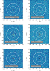 |
Fig. 1. Line integral convolution of the magnetic field, in the plane of the image. Colourmaps are for visualisation only. The black hole is marked as a black cross, and the instantaneous jet direction is shown with an orange line. The white circles have radii of 50 (dashed) and 100 (solid) kpc, respectively. In the presence of conduction, the HBI re-orients the magnetic field in a tangential configuration outside the central region. |
This evolution is shown quantitatively in Fig. 2 in the form of volume-weighted average radial profiles of the radial component of the magnetic field unit vector,  , for concentric radial shells. For all simulations, the initial conditions (dotted black line) are consistent with a tangled magnetic field (
 = 1/3). From there, the evolution diverges: without conduction,
  increases (noAGN_nocond and AGN_nocond). With conduction (noAGN_cond and AGN_cond, AGN_whistler and AGN_cr),
  decreases out to the radius where the cluster temperature profile turns over (grey vertical line, r = 358 kpc at t = 0 Gyr), that is to say within the region where the HBI can act.
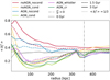 |
Fig. 2. Radial profiles of |


Low  is a clear sign of the HBI in action, which in our simulation continues to decrease
  over the full 3 Gyr of evolution. This is the case despite the fact that, unlike in Yang & Reynolds (2016) and Su et al. (2019), our jets sweep out a significant volume of the cluster centre over the 3 Gyr evolution studied here. This can be seen in Fig. 3, which shows the direction of the jet axis as a function of time. While this more isotropic injection of turbulence is effective at counteracting the HBI within the cluster centre, the limited extent of the jets’ mean values of
  still fall as low as 0.1 by r = 100 kpc, which produces an effective barrier to heat fluxes to the cluster centre. In our model, the jet has a comparatively low average spin value of about a = 0.1 (see Beckmann et al. 2019, for a discussion of the BH spin evolution), which means the spin direction is more easily adjusted than for a faster spinning BH. It is possible that a jet with a more fixed direction would be able to inject turbulence to larger radii, but this would come at the cost of affecting a smaller fraction of the core volume. We will leave an investigation into the impact of the jet model on the evolution of the magnetic field morphology to future work.
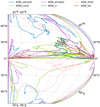 |
Fig. 3. Evolution of the jet direction for all AGN simulations over 3 Gyr of evolution. The limits of the parameter space shown account for the symmetric nature of the jet. All jets show significant re-orientation over 3 Gyr of evolution. A dot marks the jets’ final position at 3 Gyr. |
Another possibility to stabilise the HBI would be via strong magnetic fields, since the HBI growth rate is damped on scales above H ≳ 20λeβ (Quataert 2008, Eq. (33)), where β is plasma β. In our clusters, the magnetic field strength after 3 Gyr of evolution ranges from 4 − 7.5 μG in the centre to 0.5 − 1 μG at r = 100 kpc. This means H ≥ ∼640 kpc in the centre and increases with radius, so the HBI is not suppressed by magnetic tension on scales relevant to the cluster cooling flow.
Finally, whistler-wave-modulated conduction could significantly delay the HBI. As can be seen in Fig. 2,  does indeed decrease more slowly for AGN_whistler than for AGN_cond, but there is still a significant reduction in comparison to the random initial conditions. The presence of whistler waves therefore slows down, but it does not eliminate the evolution of the HBI in galaxy clusters. This is due to the fact that for realistic magnetic field strengths of a few micro Gauss in the cluster centre, plasma β in the cluster is sufficiently low such that fsat, whistler ≈ fsat early on, as can be seen in Fig. 4. It is only as the magnetic field decays away slowly throughout the simulation due to the lack of volume-filling turbulence that plasma β increases and fsat, whistler drops at late times.
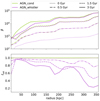 |
Fig. 4. Volume-weighted radial profiles of the mean plasma beta (top) and saturation coefficient fsat (bottom) for the two choices of fsat at three different points in time. At late times, conduction saturates at a lower value in the presence of whistler waves than in their absence. |
The conclusion that whistler-limited saturation makes only a small difference to the evolution of the HBI is in agreement with work by Berlok et al. (2021), who studied the other conduction-driven instability, the magneto-thermal instability, which is active in cluster outskirts, and they conclude that mirror instability-based suppression of thermal conduction only has a small impact. We note that using a reduced saturation coefficient is a simplified approach. A more complete treatment would be to self-consistently model the whistler-wave energy density, source, and loss terms (Drake et al. 2021), and in so doing it is likely to significantly change the conclusions on the impact of whistler waves on conduction and the HBI in galaxy clusters.
It is important to note that  increases again at small radii for both noAGN_cond and AGN_cond, but for different reasons: in AGN_cond, the AGN randomises the magnetic field in the centre for an average
  ∼1/3. In noAGN_cond, a strong cooling flow develops, which causes radial inflows. Cooling flows are also responsible for the high values of noAGN_nocond at all radii, and the late increase of
  for AGN_nocond (see Sect. 3.2).
3.2. Thermal conduction and the cooling flow
The fact that both noAGN_nocond and noAGN_cond develop a strong cooling flow can be seen in Fig. 5. Both simulations without AGN build up unrealistically large quantities of cold gas in the cluster centre as the cooling of the hot ICM proceeds unimpeded. However, noAGN_cond cools more slowly than noAGN_nocond, but the reduction in total gas mass at 3 Gyr, which is 1.0 × 10¹¹ M⊙ for noAGN_cond versus 1.4 × 10¹¹ M⊙ for noAGN_nocond, is insignificant for the total cooling flow.
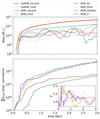 |
Fig. 5. Total cold gas mass (T < 107 K, top) and cumulative AGN energy (bottom) as a function of time. The inset shows a time series of χ = ∑EAGN, nocond/∑EAGN, cond, where ∑EAGN, nocond is the cumulative energy injected by the AGN up to time t in the simulation without conduction, while ∑EAGN, cond is the same for simulations with different conduction prescriptions. The grey-shaded region reports results from Kannan et al. (2016) and Barnes et al. (2019). The presence of an AGN strongly reduces the cooling flow, but conduction only makes a significant difference when fully isotropic. |
To further understand the potential impact of thermal conduction, we add three simulations with a fixed fc: noAGN_iso and AGN_iso have fc = 1, that is to say conduction is fully isotropic; and AGN_third also has isotropic conduction, but it uses fc = 1/3, which is equivalent to a fully tangled magnetic field. When fc is constant, any re-orientation of the magnetic field has no impact on the heat flux. It is only when conduction is isotropic (noAGN_iso), and therefore not influenced by the HBI, that conduction significantly reduces the cooling flow. This is in good agreement with the work by Wagh et al. (2014), who also show that isotropic thermal conduction significantly reduces the formation of cold gas in galaxy clusters. However, even isotropic thermal conduction is less efficient at regulating the cooling flow than AGN feedback, as can be seen by comparing noAGN_iso to any of the simulations with an AGN.
In the presence of AGN jets, cooling flows are strongly reduced as cold gas building up in the cluster activates the AGN, which prevents further cooling (see e.g., Li et al. 2015, 2017; Prasad et al. 2015; Yang & Reynolds 2016; Beckmann et al. 2019, for more details on AGN regulation of cluster cooling flows). Comparing AGN_nocond and AGN_cond in Fig. 5 shows that while the AGN effectively regulates cluster cooling and prevents a run-away cooling flow (top panel), anisotropic conduction makes little difference to the long-term evolution of the cluster.
To compare the impact of thermal conduction on the ability of the AGN to self-regulate the cluster, we define χ = ∑EAGN, nocond/∑EAGN, cond (inset, Fig. 5), where ∑EAGN(t) is the cumulative energy injected by the AGN up to time t. In our simulations, χ ≥ 1.2 – in other words the simulation without conduction requires at least 20% more cumulative AGN energy than the case with conduction – for all simulations only while t < 1 Gyr, during which the cluster is still evolving away from the initial conditions. At late times, at an average value of χ = 1.24 at t > 2 Gyr, χ remains elevated for AGN_third, but drops to ∼1 for AGN_cond and AGN_whistler. This is in contrast to Kannan et al. (2016) and Barnes et al. (2019), who report χ = 1.2 − 1.3 at all times. One possibility is that the HBI in Kannan et al. (2016) and Barnes et al. (2019) is being offset by turbulence injected by the large-scale cosmological environment. Support for this theory comes from the fact that fully tangled fields (AGN_third) in our simulations also show χ = 1.2 − 1.3. However, Yang & Reynolds (2016) used isolated clusters and also report χ ≈ 1.5. Another possibility is that as χ is very sensitive to the cluster mass (Yang & Reynolds 2016), the different χ could be due to different cluster masses or cluster profiles. A final possibility is that the higher resolution in our simulation (Δx = 531 pc compared to 1.5 − 2 kpc for other studies) is responsible for the higher fc (fc ∼ 0.2 in Yang & Reynolds 2016 vs. fc ∼ 0.1 here) and the resulting difference in χ.
Injecting a small fraction of AGN energy into cosmic rays (AGN_cr) increases the efficiency of AGN jets in self-regulating clusters (∑EAGN is reduced), but the cooling flow is only mildly affected. Further details on the impact of cosmic rays on galaxy cluster cooling flows can be found in Beckmann et al. (2022). It is only when the magnetic field becomes preferentially radial (fc → 1) that thermal conduction significantly reduces cold gas mass and cumulative AGN energy. This is in agreement with Jacob & Pfrommer (2017) who also report values of fc > 1/3 for cosmic ray and thermal conduction regulated steady-state solutions.
Such cooling flows result in significant radial mass fluxes, as can be seen in Fig. 6. Simulations without AGN show steady inflows at all radii, while those with AGN show lower net accretion rates with more disturbed patterns. The flow in simulations with AGN is less smooth due to the large-scale shocks propagating outwards from the central AGN, which disturb the contraction of the ICM as it loses thermal pressure support. In the very centre (r < 50 kpc), inflows in AGN simulations are highly variable due to the turbulence and the multi-phase nature of the gas (Beckmann et al. 2019).
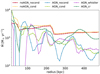 |
Fig. 6. Net mass accretion rate through concentric radial shells averaged over 3 Gyr of evolution in 500 Myr bins. The simulations without AGN show steady, smooth inflows at all radii. Simulations with AGN show, on average, lower accretion rates and more disturbed accretion patterns due to the large-scale shocks propagating outwards from the central AGN. |
It is radial mass flows that create the high values of  for noAGN_nocond in Fig. 2. For ideal MHD, field lines are ‘frozen in’, that is they are advected with the gas flow. As material falls onto the cluster centre, these mass fluxes drag the magnetic field in a radial configuration, which increases
  . This radialisation of magnetic field lines proceeds unimpeded without conduction (noAGN_nocond), but competes with the tangentialisation due to the HBI in the presence of conduction. Comparing Fig. 6 with Fig. 2 shows that simulations with strong mass fluxes have, on average, higher
  than equivalent simulations without strong mass fluxes. For example, due to the absence of a strong cooling flow,
  is lower at 100 kpc in AGN_cond than without AGN feedback (noAGN_cond) despite the HBI being very active in both. Cooling flows also explain the late rise in
  for AGN_nocond due to an excess of cold (Fig. 5), inflowing (Fig. 6) gas at t > 2.5 Gyr. Mass fluxes are high for noAGN_iso because thermal conduction efficiently extracts thermal energy from intermediate radii, which causes the gas to lose pressure support and contract.
4. Conclusions
In this paper, we investigated whether the presence of a black hole spin-driven AGN jet can counteract the HBI in the centre of massive galaxy clusters and allow for efficient thermal conduction to aid in the long-term self-regulation of cluster cooling flows. Our conclusions are as follows:
-
Spin-driven AGN feedback is able to randomise the magnetic field in the central 50 kpc of the cluster, but not outside this region.
-
Regardless of whether an AGN is included or not, the HBI remains very active in the region 50–300 kpc from the cluster centre, which reduces the effective conductivity to values as low as fc = 0.1 of Spitzer conductivity.
-
Such low levels of thermal conduction have no significant influence on the cluster cooling flow, or the AGN self-regulation thereof.
-
Whistler-wave-driven saturation of thermal conduction reduces the magnitude of the HBI in galaxy clusters, but does not prevent it.
-
Even if the HBI was inefficient and the magnetic field remained tangled, the resulting effective conductivity of fc = 1/3 Spitzer is not sufficiently high to influence the AGN self-regulated cooling flow.
-
Only very high values of fc, which would require predominantly radial magnetic fields, transport sufficient thermal energy to reduce the cluster cooling flow.
Our set of idealised simulations have demonstrated the inability of AGN jets alone to re-randomise the magnetic field after it has been tangentially aligned by the HBI, and, hence, to restore significant thermal conduction on cluster scales. We have shown that thermal conduction does affect the morphology of the magnetic field, which in turn could have important consequences on where cosmic ray energy is deposited in the cluster (see Beckmann et al. 2022). How the magnetic field evolves strongly depends on how conduction is modelled, and on the initial conditions of the magnetic field. We defer a more detailed study of the impact of magnetic field morphology on the evolution of galaxy clusters to future work, together with a study of the contribution of other sources of turbulence beyond AGN jets, such as large-scale inflows, stirring by satellites, and other substructures (Ruszkowski & Oh 2011; Bourne & Sijacki 2017). Other phenomena to be considered are anisotropic thermal pressure due to Braginskii viscosity (Kunz et al. 2011).
Acknowledgments
We would like to thank the referee for their constructive comments. RSB And YD designed the project, RSB, YD and AP developed the code, interpreted results and wrote the paper. RSB designed, executed and processed the suite of simulations. FLP and VO contributed to discussion and interpretation of results. This work was supported by the ANR grant LYRICS (ANR-16-CE31-0011) and was granted access to the HPC resources of CINES under the allocations A0080406955 and A0100406955 made by GENCI. This work has made use of the Infinity Cluster hosted by Institut d’Astrophysique de Paris. We thank Stéphane Rouberol for smoothly running this cluster for us. Visualisations in this paper were produced using the YT PROJECT (Turk et al. 2011) and CARTOPY (Met Office 2015).
References
- Andreon, S., Wang, J., Trinchieri, G., Moretti, A., & Serra, A. L. 2017, A&A, 606, A24 [NASA ADS] [CrossRef] [EDP Sciences] [Google Scholar]
- Barnes, D. J., Kannan, R., Vogelsberger, M., et al. 2019, MNRAS, 488, 3003 [CrossRef] [Google Scholar]
- Beckmann, R. S., Dubois, Y., Guillard, P., et al. 2019, A&A, 631, A60 [EDP Sciences] [Google Scholar]
- Beckmann, R. S., Dubois, Y., Pellisier, A., et al. 2022, A&A, 665, A129 [NASA ADS] [CrossRef] [EDP Sciences] [Google Scholar]
- Berlok, T., Quataert, E., Pessah, M. E., & Pfrommer, C. 2021, MNRAS, 504, 3435 [NASA ADS] [CrossRef] [Google Scholar]
- Binney, J., & Tabor, G. 1995, MNRAS, 276, 663 [NASA ADS] [Google Scholar]
- Bogdanović, T., Reynolds, C. S., Balbus, S. A., & Parrish, I. J. 2009, ApJ, 704, 211 [CrossRef] [Google Scholar]
- Bourne, M. A., & Sijacki, D. 2017, MNRAS, 472, 4707 [NASA ADS] [CrossRef] [Google Scholar]
- Cowie, L. L., & McKee, C. F. 1977, ApJ, 211, 135 [NASA ADS] [CrossRef] [Google Scholar]
- Dashyan, G., & Dubois, Y. 2020, A&A, 638, A123 [EDP Sciences] [Google Scholar]
- Drake, J. F., Pfrommer, C., Reynolds, C. S., et al. 2021, ApJ, 923, 245 [NASA ADS] [CrossRef] [Google Scholar]
- Dubois, Y., & Commerçon, B. 2016, A&A, 585, A138 [NASA ADS] [CrossRef] [EDP Sciences] [Google Scholar]
- Dubois, Y., Devriendt, J., Slyz, A., & Teyssier, R. 2012, MNRAS, 420, 2662 [Google Scholar]
- Dubois, Y., Volonteri, M., Silk, J., Devriendt, J., & Slyz, A. 2014, MNRAS, 440, 2333 [Google Scholar]
- Dubois, Y., Beckmann, R., Bournaud, F., et al. 2021, A&A, 651, A109 [NASA ADS] [CrossRef] [EDP Sciences] [Google Scholar]
- Fabian, A. C. 1994, ARA&A, 32, 277 [Google Scholar]
- Fromang, S., Hennebelle, P., & Teyssier, R. 2006, A&A, 457, 371 [NASA ADS] [CrossRef] [EDP Sciences] [Google Scholar]
- Gaspari, M., Ruszkowski, M., & Oh, S. P. 2013, MNRAS, 432, 3401 [NASA ADS] [CrossRef] [Google Scholar]
- Jacob, S., & Pfrommer, C. 2017, MNRAS, 467, stx131 [CrossRef] [Google Scholar]
- Kannan, R., Vogelsberger, M., Pfrommer, C., et al. 2016, ApJ, 837, L18 [Google Scholar]
- Kimm, T., Cen, R., Devriendt, J., Dubois, Y., & Slyz, A. 2015, MNRAS, 451, 2900 [CrossRef] [Google Scholar]
- Komarov, S., Schekochihin, A., Churazov, E., & Spitkovsky, A. 2018, J. Plasma Phys., 84, 905840305 [NASA ADS] [CrossRef] [Google Scholar]
- Kunz, M. W., Schekochihin, A. A., Cowley, S. C., Binney, J. J., & Sanders, J. S. 2011, MNRAS, 410, 2446 [NASA ADS] [CrossRef] [Google Scholar]
- Leccardi, A., & Molendi, S. 2008, A&A, 487, 461 [NASA ADS] [CrossRef] [EDP Sciences] [Google Scholar]
- Li, Y., Bryan, G. L., Ruszkowski, M., et al. 2015, ApJ, 811, 73 [Google Scholar]
- Li, Y., Ruszkowski, M., & Bryan, G. G. L. 2017, ApJ, 847, 106 [NASA ADS] [CrossRef] [Google Scholar]
- Maccio, A. V., Dutton, A. A., Van Den Bosch, F. C., et al. 2007, MNRAS, 378, 55 [NASA ADS] [CrossRef] [Google Scholar]
- McCourt, M., Parrish, I. J., Sharma, P., & Quataert, E. 2011, MNRAS, 413, 1295 [NASA ADS] [CrossRef] [Google Scholar]
- McKinney, J. C., Tchekhovskoy, A., & Blandford, R. D. 2012, MNRAS, 423, 3083 [Google Scholar]
- Met Office. 2015, https://doi.org/10.5281/zenodo.5842769 [Google Scholar]
- Miyoshi, T., & Kusano, K. 2005, J. Comput. Phys., 208, 315 [NASA ADS] [CrossRef] [Google Scholar]
- Narayan, R., & Medvedev, M. V. 2001, ApJ, 562, L129 [NASA ADS] [CrossRef] [Google Scholar]
- Navarro, J. F., Frenk, C. S., & White, S. D. M. 1997, ApJ, 490, 493 [Google Scholar]
- Parrish, I. J., Quataert, E., & Sharma, P. 2009, ApJ, 703, 96 [NASA ADS] [CrossRef] [Google Scholar]
- Parrish, I. J., McCourt, M., Quataert, E., & Sharma, P. 2012, MNRAS, 422, 704 [NASA ADS] [CrossRef] [Google Scholar]
- Phipps, F., Bogdán, Á., Lovisari, L., et al. 2019, ApJ, 875, 141 [NASA ADS] [CrossRef] [Google Scholar]
- Prasad, D., Sharma, P., & Babul, A. 2015, ApJ, 811, 108 [Google Scholar]
- Quataert, E. 2008, ApJ, 673, 758 [NASA ADS] [CrossRef] [Google Scholar]
- Roberg-Clark, G. T., Drake, J. F., Reynolds, C. S., & Swisdak, M. 2016, ApJ, 830, L9 [Google Scholar]
- Rosen, A., & Bregman, J. N. 1995, ApJ, 440, 634 [NASA ADS] [CrossRef] [Google Scholar]
- Ruszkowski, M., & Begelman, M. C. 2002, ApJ, 581, 223 [NASA ADS] [CrossRef] [Google Scholar]
- Ruszkowski, M., & Oh, S. P. 2010, ApJ, 713, 1332 [NASA ADS] [CrossRef] [Google Scholar]
- Ruszkowski, M., & Oh, S. P. 2011, MNRAS, 414, 1493 [NASA ADS] [CrossRef] [Google Scholar]
- Ruszkowski, M., Lee, D., Brüggen, M., Parrish, I., & Oh, S. P. 2011, ApJ, 740, 81 [NASA ADS] [CrossRef] [Google Scholar]
- Santos, S. D. 2000, MNRAS, 323, 930 [Google Scholar]
- Sarazin, C. L. 1986, Rev. Mod. Phys., 58, 1 [Google Scholar]
- Sharma, P., Quataert, E., Hammett, G. W., & Stone, J. M. 2007, ApJ, 667, 714 [NASA ADS] [CrossRef] [Google Scholar]
- Spitzer, L., & Härm, R. 1953, Phys. Rev., 89, 977 [Google Scholar]
- Su, K.-Y., Hopkins, P. F., Hayward, C. C., et al. 2019, MNRAS, 487, 4393 [NASA ADS] [CrossRef] [Google Scholar]
- Sutherland, R. S., & Dopita, M. A. 1993, ApJS, 88, 253 [Google Scholar]
- Teyssier, R. 2002, A&A, 385, 337 [CrossRef] [EDP Sciences] [Google Scholar]
- Teyssier, R., Fromang, S., & Dormy, E. 2006, J. Comput. Phys., 218, 44 [NASA ADS] [CrossRef] [Google Scholar]
- Tucker, W. H., & Rosner, R. 1983, ApJ, 267, 547 [CrossRef] [Google Scholar]
- Turk, M. J., Smith, B. D., Oishi, J. S., et al. 2011, ApJS, 192, 9 [NASA ADS] [CrossRef] [Google Scholar]
- Urban, O., Werner, N., Allen, S. W., Simionescu, A., & Mantz, A. 2017, MNRAS, 470, 4583 [Google Scholar]
- Wagh, B., Sharma, P., & McCourt, M. 2014, MNRAS, 439, 2822 [CrossRef] [Google Scholar]
- Yang, H.-Y. K., & Reynolds, C. S. 2016, ApJ, 818, 181 [NASA ADS] [CrossRef] [Google Scholar]
All Tables
All Figures
|
Fig. 1. Line integral convolution of the magnetic field, in the plane of the image. Colourmaps are for visualisation only. The black hole is marked as a black cross, and the instantaneous jet direction is shown with an orange line. The white circles have radii of 50 (dashed) and 100 (solid) kpc, respectively. In the presence of conduction, the HBI re-orients the magnetic field in a tangential configuration outside the central region. |
| In the text | |
|
Fig. 2. Radial profiles of |
| In the text | |
|
Fig. 3. Evolution of the jet direction for all AGN simulations over 3 Gyr of evolution. The limits of the parameter space shown account for the symmetric nature of the jet. All jets show significant re-orientation over 3 Gyr of evolution. A dot marks the jets’ final position at 3 Gyr. |
| In the text | |
|
Fig. 4. Volume-weighted radial profiles of the mean plasma beta (top) and saturation coefficient fsat (bottom) for the two choices of fsat at three different points in time. At late times, conduction saturates at a lower value in the presence of whistler waves than in their absence. |
| In the text | |
|
Fig. 5. Total cold gas mass (T < 107 K, top) and cumulative AGN energy (bottom) as a function of time. The inset shows a time series of χ = ∑EAGN, nocond/∑EAGN, cond, where ∑EAGN, nocond is the cumulative energy injected by the AGN up to time t in the simulation without conduction, while ∑EAGN, cond is the same for simulations with different conduction prescriptions. The grey-shaded region reports results from Kannan et al. (2016) and Barnes et al. (2019). The presence of an AGN strongly reduces the cooling flow, but conduction only makes a significant difference when fully isotropic. |
| In the text | |
|
Fig. 6. Net mass accretion rate through concentric radial shells averaged over 3 Gyr of evolution in 500 Myr bins. The simulations without AGN show steady, smooth inflows at all radii. Simulations with AGN show, on average, lower accretion rates and more disturbed accretion patterns due to the large-scale shocks propagating outwards from the central AGN. |
| In the text | |
Current usage metrics show cumulative count of Article Views (full-text article views including HTML views, PDF and ePub downloads, according to the available data) and Abstracts Views on Vision4Press platform.
Data correspond to usage on the plateform after 2015. The current usage metrics is available 48-96 hours after online publication and is updated daily on week days.
Initial download of the metrics may take a while.