| Issue |
A&A
Volume 665, September 2022
|
|
|---|---|---|
| Article Number | A18 | |
| Number of page(s) | 11 | |
| Section | Atomic, molecular, and nuclear data | |
| DOI | https://doi.org/10.1051/0004-6361/202243875 | |
| Published online | 06 September 2022 | |
Atomic radiative data for oxygen and nitrogen for solar photospheric studies
1
Department of Physics, Western Michigan University,
Kalamazoo,
MI 49008
USA
e-mail: This email address is being protected from spambots. You need JavaScript enabled to view it.
2
Max Planck Institute for Astronomy,
69117
Heidelberg, Germany
3
Physique Atomique et Astrophysique, Université de UMONS,
7000
Mons, Belgium
4
IPNAS, Université de Liège,
4000
Liège, Belgium
Received:
26
April
2022
Accepted:
27
June
2022
Abstract
Aims. Our recent reanalysis of the solar photospheric spectra with non-local thermodynamic equilibrium (non-LTE) models resulted in higher metal abundances compared to previous works. When applying the new chemical abundances to standard solar model calculations, the new composition resolves the long-standing discrepancies with independent constraints on the solar structure from helioseismology.
Methods. Critical to the determination of chemical abundances is the accuracy of the atomic data, especially the f values, used in the radiative transfer models. Here we describe, in detail, the calculations of f values for neutral oxygen and nitrogen used in our non-LTE models.
Results. Our calculations of f values are based on a multi-method, multi-code approach and they are the most detailed and extensive of its kind for the spectral lines of interest. We also report in this paper the details of an extensive R-matrix calculation of photoionization cross sections for oxygen.
Conclusions. Our calculation resulted in reliable f values with well-constrained uncertainties. We compare our results with previous theoretical and experimental determinations of atomic data. We also quantify the influence of adopted photoionization cross sections on the spectroscopic estimate of the solar O abundance, using data from different sources. We confirm that our 3D non-LTE value is robust and unaffected by the choice of photoionization data, contrary to the recent claim made by Nahar.
Key words: atomic data / line: formation / Sun: abundances / Sun: photosphere
© M. A. Bautista et al. 2022
 Open Access article, published by EDP Sciences, under the terms of the Creative Commons Attribution License (https://creativecommons.org/licenses/by/4.0), which permits unrestricted use, distribution, and reproduction in any medium, provided the original work is properly cited.
This article is published in open access under the Subscribe-to-Open model. This email address is being protected from spambots. You need JavaScript enabled to view it. to support open access publication.
1 Introduction
Among elements heavier than helium, the abundances of carbon (C), nitrogen (N), and oxygen (O) amount to about two-thirds of all elements by mass. Moreover, O is the major contributor to the opacity in the solar interior that determines the transport of energy and thus the interior structure of the Sun. Determining accurate abundances of these elements is critically important to understand the solar structure and evolution. In addition, measurements of CNO abundances in stars are crucial to address a variety of different problems in modern astrophysics, including but not limited to studies of Galactic chemical evolution and enrichment by asymptotic giant branch stars (Bensby et al. 2014; Bergemann et al. 2018; Schuler et al. 2021), multiple populations in stellar clusters (Tautvaišiene et al. 2022), the structure of proto-planetary disks (Turrini et al. 2021), as well as planet formation and planetary atmospheres (Borsa et al. 2021).
The most reliable solar chemical abundances are obtained from the solar photospheric spectrum (Lodders 2019). Regarding the solar O abundance, various groups have studied it in different ways. Grevesse & Sauval (1998) deduced an O photospheric abundance of 8.83 ± 0.06 dex, based on 1D local thermodynamic equilibrium (LTE) methods. By contrast, recent estimates from detailed non-LTE analysis, with 3D radiation-hydrodynamics (RHD) simulations of convection, are log A(O) = 8.69 ± 0.04 dex (Asplund et al. 2021) and log A(O) = 8.76 ± 0.07 dex (Caffau et al. 2008). The former abundance leads to solar interior opacities that are too low to satisfy the standard solar model calculations (Serenelli et al. 2009, 2011; Villante & Serenelli 2020). This is because these opacities lead to a predicted internal structure of the present-day Sun, with a sound speed profile, depth of the convective envelope, and surface He abundance, which is contradicted by independent constraints on its structure obtained from helioseismology.
Bergemann et al. (2021) reanalyzed the solar photospheric O abundance using revised and more complete atomic data, as well as non-LTE calculations with 1D hydrostatic (MARCS) and 3D radiation-hydrodynamics and magneto-hydrodynamics simulations of the solar atmosphere from the STAGGER (Collet et al. 2011) and BIFROST (Gudiksen et al. 2011) codes. The Bergemann et al. (2021) analysis also takes the influence of the chromosphere into account. By comparing the theoretical line profiles with high-resolution, R ≈ 700 000, spatially resolved spectra of the Sun, they found log A(O) = 8.74 ± 0.03 dex from the permitted O I lines at 777 nm and log A(O) = 8.77 ± 0.05 dex from the forbidden [O I] line at 630 nm. In Magg et al. (2022), we extended this approach to estimate the abundances of all important chemical elements in the solar photosphere. This includes a new estimate of the N abundance based on newly calculated oscillator strengths. The revised abundances are higher compared to those reported in the previous non-LTE analysis by Asplund et al. (2021). Our revised values yield solar interior opacities in much better agreement with the helioseismic constraints.
Key parameters in all chemical abundance determinations are the radiative transition probabilities adopted since errors in the adopted A values directly affect the derived abundances. The vast majority of A values come from theoretical calculations and the differences in the results published by different authors often exceed the reported uncertainties. Uncertainties in calculated values can be broadly categorized as statistical and systematic. The former shall include the dispersion in numerical results, arising from different treatments of the atomic potential and the optimization techniques of atomic orbitals. The systematic uncertainties are much more difficult to predict and to quantify because they result from incomplete descriptions of atomic states. Such descriptions of states are generally done by configuration interaction (CI) and/or level mixing schemes that lead to expansions, which must be truncated by computational limitations.
In this paper, we present the details of the calculations of radiative transition probabilities for N and O, which contributed to a significant revision of the solar chemical abundances of these elements. We are especially concerned with the uncertainties of the derived transitions rates. To this end, we have carried out large, exhaustive calculations of f values for the particular O and N lines measured in the observed solar spectra. For these calculations, we use three different and independent theoretical methods and compare the results in detail.
As we were preparing this publication, Nahar (2022) criticized the atomic data used in Bergemann et al. (2021) and put into question our new 3D non-LTE estimate of the solar O abundance. Nahar’s criticism especially focuses on the photoionization cross sections of O I states. Thus, we include here a detailed description of our cross sections. Further, we demonstrate how the differences in the cross sections influence the solar spectroscopic models and resulting solar O abundance using independent sources of photoionization cross sections.
2 Transition probabilities and f values
In this section we describe the calculation of radiative transition probabilities. We used four different computer codes employing different theoretical approaches. These are: (i) AUTOSTRUCTURE (Badnell 2011) which is based on the Thomas-Fermi-Dirac-Amaldi central potential; (ii) the R-matrix method impletented in the RMATRX package (Berrington et al. 1995); (iii) the HFR+CPOL approach based on the pseudo-relativistic Hartree-Fock (HFR) method initially introduced by Cowan (1981) and modified to take core-polarization effects into account (Quinet et al. 1999, 2002); and (iv) the GRASP2018 code (Froese Fischer et al. 2019) based on the fully relativistic multiconfiguration Dirac-Hartree-Fock (MCDHF) method (Grant 2007; Froese Fischer et al. 2019).
In providing the most accurate radiative rates and f values for transitions of O I and N I, we also need to provide reliable uncertainty estimates for these rates. The specific lines of interest for O are λλ7771.94, 7774.42,  and for N are
  .
.
2.1 AUTOSTRUCTURE calculations
AUTOSTRUCTURE solves the Breit-Pauli Schrödinger equation with a scaled Thomas–Fermi–Dirac (TFD) central-field potential to generate orthonormal atomic orbitals. Configuration interaction (CI) atomic state functions are built using these orbitals. The scaling factors for each orbital are optimized in a multiconfiguration variational procedure minimizing a sum over LS term energies or a weighted average of LS term energies. Perturbative corrections, that is term energy corrections (TECs), are applied to the multi-electronic Hamiltonian, which adjusts theoretical LS term energies closer to the centers of gravity of the available experimental multiplets. A final empirical correction, that is level energy correction (LEC), is applied to reproduce level energy separations when computing gf values and transitions probabilities.
We carried out numerous calculations, systematically adding additional configurations to the CI expansion. In doing so, we observed the evolution of the gf values as they reached convergence and we were able to quantify statistical and systematic uncertainties in the final rates. We aimed to include, within computational limits, all configurations that contribute to the rates for the transitions of interest, while maintaining good overall representation for the entire atomic system.
It should be noted that many configurations in the CI expansion that contribute to a particular transition rate may not influence the energies of the levels involved in any significant way. Thus, one cannot generally assess the importance of including specific configurations to the transitions of interest based on only the predicted level energies. Instead, one needs to carry out the full calculation, including orbital optimizations, TECs and LECs, up to computing the actual radiative rates. This makes the work presented here computationally intensive. Orbital optimization often requires numerous calculations of the atomic model. After each calculation, one must compare the predicted energies with experimental values in detail, compute differences, and find the term identification numbers and level idensitifcation numbers assigned by the code, which change from model to model. Once the potential is satisfactorily optimized, one uses the difference between predicted and experimental term-averaged energies for a new calculation with TECs. At this stage, the LECs are produced from the difference with experiment in fine-structure level energies, and a final large calculation of all transition rates is carried out. This procedure has to be automatized because of the very large datasets involved, and in order to minimize errors caused by inspection by eye. Therefore, a Python code is used, which semi-automatically generates AUTOSTRUCTURE input files, reads the output files, compares them with experimental data, and produces TEC and LEC factors.
We started the computations by selecting the orbitals that need to be accounted for in our calculations. By inspection of the results obtained with CI expansion of the form 2s22p3nl for 0 and 2s22p2nl for N, we find that only orbitals with n ≤ 5 and l ≤ 3 for O and n ≤ 6 and l ≤ 4 for N make significant contributions to the transitions of interest. These orbitals define finite sets of possible configurations to be included in our CI expansions. However, all together these amount to thousands of configurations for each atom and including them all at once would exceed the available computational resources at the present. Therefore, our approach was to start from a relatively small CI expansion which yields a reasonably good representation of levels up to those of interest. Then, we progressively added sets of configurations by single-, double-, and triple-electron promotions. At each stage we retained only those new configurations that affect the transition rates of interest and discarded unimportant configurations. This way, we sought to obtain the most accurate rates possible while keeping the CI expansion manageable. Below we present details of the calculations for each species and the results.
CI expansions used in the calculation of radiative rates of neutral O.
Comparison of experimental and predicted ab initio energies in Ryd from our different AUTOSTRUCTURE target expansions for O.
2.1.1 O
We started with a 15-configuration expansion we refer to as CI-A. This expansion includes orbitals up to principal quantum number n = 4 and angular momentum l ≤ 2, as shown in Table 1. This expansion gives a very reasonable structure in terms of energies (see Table 2). The theoretical energies shown in this table are ab initio energies, prior to term and level energy corrections. One can see that the CI-A expansion gives acceptable energies (within ~ 10% from experiment) for terms from the 2p4 configuration. The energies of terms from the 2p33s and 2p34s configurations are very good. The expansion also gives good energies for the lowest terms from the 2p33p and 2p33d configurations, but the energies of the higher terms are significantly overestimated. This is because the angular momentum splitting of these configurations is inaccurate in the ab initio representation. Nonetheless, the CI-A expansion gives term energies within ~2% of experiment for the states 2p33s 5So and 2p33p5P. Moreover, the representation of all terms is expected to be improved by using TECs.
Expansion CI-B extends the original expansion by one-electron promotions from the 2s orbital. Expansion CI-C extends CI-B by configurations with two electrons in n = 4. These expansions change neither the atom’s description nor the transition rates of interest (see Fig. 1) in a significant way.
Expansions CI-D and CI-E extend the original expansion by two electron promotions from 2s. Again, this results in only small changes to the atomic structure and changes to the transition rates of less than 1%. If anything, these expansions lead to slight increases in the difference between length and velocity gauges of the gf values of the dipole transitions.
In expansions CI-F, CI-G, and CI-H, we explore additional two- and three-electron promotions from 2s and 2p orbital to n = 3 and 4 valence orbitals. In all cases, the energies remain essentially unchanged and so are the transitions rates.
Expansions CI-I and CI-J, with 49 and 106 configurations, respectively, are the largest we ran. Both of these include n = 5 orbitals. In CI-I, we included configurations with up to three electron promotions, with one electron from 2s and up to two electrons from 2p. In CI-J we have configurations with up to four electron promotions. The additional configurations yield no large changes to the predicted atomic structure, but the difference between length and velocity gauges of the gf values is reduced from ~15% to ~9<%.
Figure 1 shows the gf values for the λ7771 dipole-allowed line. Other lines of this multiplet have the same behavior, thus we do not show them. Both length and velocity gauges of the gf values as obtained with AUTOSTRUCTURE are shown in the figure. TECs and LECs have been included in all calculations. Without them, the scatter in the obtained rates is spuriously larger than shown in the figure. The results of our R-matrix, HFR+CPOL, and MDCHF calculations are also shown here and they are discussed below. It can be seen that the gf values for this transition are remarkably stable and the length and velocity gauges agree well (within ~ 10%). We conclude that the transition rate is converged and reliable.
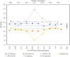 |
Fig. 1 gf values for the O I λ7771 line. The results of all different model calculations are shown in increasing order of complexity from left to right. The values depicted are AUTOSTRUCTURE length (AUTOSS (L)) and velocity (AUTOSS (V)) gauges as circles and square points, respectively; MCDHF Babushkin (MCDHF (B)) and Coulomb (MCDHF (C)) gauges are shown with diamond and triangular points, respectively; HFR+CPOL is the horizonal long-dashed line; and R-matrix length (R-matrix(L)) and velocity (R-matrix(V)) gauges are shown with dot-dashed lines. The point with error bars at the right end of the plot depicts our recommended gf fvalue for the transitions and its estimated uncertainty. |
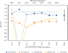 |
Fig. 2 gf values for the N I λ8683 line. The different point types and lines are the same as in Fig. 1. |
2.1.2 N
The N transitions of interest here converge much more slowly than the O lines. To achieve reliable gf values with AUTOSTRUCTURE, we had to progressively increase the size of the CI expansion to include up to 355 configurations. The different expansions used here are described in Table 3 and the resultant, uncorrected energies from these expansions are presented in Table 4.
All expansions yield acceptable term energies, within ~10% of the experimental values, with the exception of energies for the 2s22p3 2Po term from the CI-A and CI-B expansions. These two expansions overestimate the energy split among terms of the ground configuration 2s2 2p3. Unaccounted electron-electron correlations are at fault here, but this was resolved by adding configurations with two-electron promotions from the 2s orbital. This was done in CI-C and all larger expansions. For all expansions, we find that the predicted energies for excited configurations are systematically underestimated. This is due to strong relaxation effects of the 2p orbital. This is likely to introduce error in the calculated transition rates, though TECs mitigate these errors in sufficiently large CI expansions.
When computing radiative rates and gf values, we find significant discrepancies between the length and velocity gauges. The velocity gauge values, which preferentially weigh the small radius part of the wavefunctions, are often less reliable than the length gauge. Thus, we consider the former set of values for the uncertainty estimates.
Figures 2 and 3 depict the evolution of the gf values for the N I λ8683 and λ8629 lines, respectively. We see that the value for the λ8683 line is scattered between 1.4 and 1.6, while the scatter for the λ8629 lines ranges from 1.0 to 1.2. From the minimum expansion CI-A to CI-B, we see that both gf values sharply increase by more than 10%, as a result of two-electron promotions from the 2p orbital. Then, two-electron promotions from the 2s, included in expansion CI-C, bring the gf values down again. Simultaneous promotions from 2s and 2p, included in configurations CI-D and CI-E, seem to make the values to converge to about 1.47 and 1.03, respectively. However, adding n = 5 orbitals in expansions CI-F and CI-G changes the gf values again to 1.40 and 1.16. These last expansions, with 126 and 355 configurations, yield nearly identical results and we expect them to have reached convergence.
CI expansions used in the calculation of radiative rates of neutral N.
2.2 R-matrix
The R-matrix method allows for the calculation of bound level energies and g f values for electric dipole transitions. Here, the wavefunctions of the bound levels were constructed as CI expansions of basis state functions built using the close coupling approximation. This method is implemented in the RMTRX computer package (Berrington et al. 1995).
We computed O gf values for the transitions of interest from the same calculation carried out for photoionization cross sections. The details of this calculation are presented in Sect. 4. As a verification of the quality of the calculations, Table 5 compares the ab initio predicted bound energies of the levels of interest with experimental energy values compiled by NIST (Kramida et al. 2021). It can be seen that the predicted energies of the 3s 5S2 level and 3p 5Pj levels are underestimated by about 6% and <5%, repectively. This is considered good accuracy for predicted bound state energies and provides support to the reliability of the results.
R-matrix calculations of gf values have the advantage of including a lot of CI very efficiently. The down side, though, is that the calculations are too demanding to allow for detailed follow-up of the convergence of specific transitions.
Comparison of experimental and predicted ab initio energies in Ryd from our different AUTOSTRUCTURE target expansions for N.
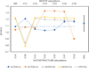 |
Fig. 3 gf values for the N I λ8629 line. The different point types and lines are the same as in Fig. 1. |
Comparison of experimental and predicted energies in Ryd from our R-matrix, HFR, and MCDHF calculations for O.
Comparison of experimental and predicted energies in Ryd from our HFR and MCDHF calculations for N.
2.3 Pseudo-relativistic Hartree-Fock + core-polarization calculations
Another approach used to compute oscillator strengths in O I and N I was the HFR+CPOL method. This consists of the pseudo-relativistic Hartree-Fock (HFR) method (Cowan 1981) and it was later modified to take core-polarization effects into account (Quinet et al. 1999, 2002). The computational strategies developed for each atomic system are detailed in the following.
Tables 5 and 6 compare the calculated energies of the levels of interest in O and N, respectively, with experimental energies from NIST (Kramida et al. 2021). The details of the calculations are described hereafter.
2.3.1 O
In the case of neutral O, the valence-valence interactions were considered among a set of configurations including 2p4, 2p3nl (with nl up to 6h) and all single and double (SD) excitations from 2s, 2p to 3s, 3p, 3d orbitals while the core-valence interactions involving the 1s subshell were modeled by a core-polarization potential. More precisely, the 2s22p4, 2s22p3np (n = 3-6), 2s22p3nf (n = 4–6), 2s22p36h, 2s22p23s2, 2s22p23p2, 2s22p23d2, 2s22p23s3d, 2s22p3p3, 2s22p3s23p,2s22p3p3d2, 2s22p3s3p3d, 2s2p43s, 2s2p43d, 2s2p33s3p, 2s2p33p3d, 2p6, 2p533p, 22p43s23, 2p43p2, 2p43d2, 2p43s3d, 2p33p3, 2p33s23p, 2p33p3d2, 2p33s3p3d even-parity configurations, and the 2s22p3ns (n = 3-6), 2s22p3nd (n = 3-6), 2s22p3ng (n = 5-6), 2s22p23s3p, 2s22p23p3d, 2s22p3d3, 2s22p3s23d, 2s22p3s3p2, 2s22p3p23d, 2s22p3s3d2, 2s2p5, 2s2p43p, 2s2p33s2, 2s2p33p2, 2s2p33d2, 2s2p33s3d, 2p53s, 2p53d, 2p43s3p, 2p43p3d, 2p33d3, 2p33s23d, 2p33s3p2, 2p33p23d, 2p33s3d2 odd-parity configurations were explicitly included in the HFR physical model. Core-valence correlations were modeled by a core-polarization potential corresponding to a He-like O VII ionic core with a dipole polarizability αd = 0.0026  (Johnson et al. 1983) and a cut-off radius rc = 0.198 a0. The latter value corresponds to the calculated HFR value of <1s|r| 1s> of the outermost core orbital (1s). In addition, a semi-empirical fitting of the energy levels was performed in order to reduce the discrepancies between the calculated and experimental wavelengths for the three transitions of interest.
Figure 1 depicts our HFR+CPOL gf value with a long-dashed horizontal line. This lays right in between the length and velocity gauges obtained with AUTOSTRUCTURE and the Babushkin (B) and Coulomb (C) gauges obtained with MCDHF.
2.3.2 N
For the calculations in neutral N, the following configurations were included in the HFR model: 2s22p3, 2s22p2np (n = 3-6), 2s22p2nf (n = 4-6), 2s22p26h, 2s22p3s2, 2s22p3p2, 2s22p3d2, 2s22p3s3d, 2s23p3, 2s23s23p,2s23p3d2, 2s23s3p3d, 2s2p33s, 2s2p33d, 2s2p23s3p, 2s2p23p3d, 2p5, 2p43p, 2p33s2, 2p33p2, 2p33d2, 2p33s3d, 2p23p3, 2p23s23p, 2p23p3d2, 2p23s3p3d (odd parity), and 2s22p2ns (n = 3–6), 2s22p2nd (n = 3-6), 2s22p2ng (n = 5–6), 2s22p3s3p, 2s22p3p3d, 2s23d3, 2s23s23d, 2s23s3p2, 2s23p23d, 2s23s3d2, 2s2p4, 2s2p33p, 2s2p23s2, 2s2p23p2, 2s2p23d2, 2s2p23s3d, 2p43s, 2p43d, 2p33s3p, 2p33p3d, 2p23d3, 2p23s23d, 2p23s3p2, 2p23p23d, 2p23s3d2 (even parity). The core-polarization parameters corresponding to a He-like N VI ionic core were chosen as  (Johnson et al. 1983) and rc = 0.228 a0. As for O, a semi-empirical adjustment to the computed energies was performed in order to reproduce the experimental wavelengths for the two N I lines of interest as well as possible.
The HFR+CPOL results for both lines of interest are shown in Figs. 2 and 3 by long-dashed horizontal lines. The HFR+CPOL gf value for the λ 8683 line are 10% lower than the values found with AUTOSTRUCTURE and MCDHF, the HFR+CPOL, while the value for the λ 8629 line is ~10% higher. We consider this level of agreement to be satisfactory, given the complexity of these N transitions. However, it is clear the level of uncertainty of the N lines is larger than for the O lines.
3 Multiconfiguration Dirac-Hartree-Fock calculations
We also calculated the radiative parameters using the purely relativistic multiconfiguration Dirac-Hartree-Fock (MCDHF) method developed by Grant (2007) and Froese Fischer et al. (2016). This is implemented in the General Relativistic Atomic Structure Program (GRASP) and we used the latest version of this code, GRASP2018 (Froese Fischer et al. 2016).
Different physical models were applied to each atom in order to optimize the wave functions and the corresponding energy levels by gradually increasing the basis of configuration state functions (CSFs), and thus taking more correlations into account. To begin with, a multireference (MR) of configurations was chosen as being composed of 2s22pk, 2s22pk−13s, 2s22pk−13p and 2s22pk−13d with k = 3, 4 for N I and O I, respectively. Then, valence-valence (VV) models, in which SD excitations of valence electrons – that is occupied subshells of configurations from the MR except the 1s orbital – to a set of active orbitals were considered in order to generate the CSF expansions. These sets of active orbitals were gradually extended up to 9s, 9p, 9d, 6f, 6g, and 6h. In each VV model, we added core-valence (CV) correlations by considering single excitations from the 1s orbital to those characterizing the MR configurations. It was found that the CV correlations are negligible (i.e., the results of the VV and CV models are essentially identical) for the transitions of interest in both O and N. Thus, while we describe both sets of models, we only present the CV model results and refer to them as MCDHF values. Finally, the high-order relativistic effects, that is the Breit interaction, QED self-energy, and vacuum polarization effects, were incorporated in the relativistic configuration interaction (RCI) step of the GRASP2018 package. The details of the MCDHF calculations carried out in O and N atoms are given below.
Tables 5 and 6 compare the calculated energies of the levels of interest with experimental energies from NIST (Kramida et al. 2021). For calculated energies, we take those from the largest models described below.
3.1 O
In neutral O, the MR consisted in 2s22p4, 2s22p33s, 2s22p33p and 2s22p33d configurations, from which all the levels were considered to optimize the 1s, 2s, 2p, 3s, 3p, and 3d orbitals. A first VV model (VV1) was built by adding - to the MR configurations – SD excitations from 2s, 2p, 3s, 3p, and 3d to the {nl,n′l′,…} active set of orbitals, where n, n′,… stand for the maximum principal quantum numbers corresponding to the l, l′,… orbital quantum numbers. In the first VV model (VV1), we considered {4s,4p,4d,4f} to be an active set. In this step, only the new orbitals were optimized, the other ones being kept to their values obtained before. The same strategy was used to build more elaborate VV models by successively considering the following sets of active orbitals: {5s,5p,5d,5f,5g} for VV2, {6s,6p,6d,6f,6g,6h} for VV3, {7s,7p,7d,6f,6g,6h} for VV4, {8s,8p,8d,6f,6g,6h} for VV5, and {9s,9p,9d,6f,6g,6h} for VV6. For each of these VV models, core-valence correlations were added by means of single excitations from the 1s orbital to the active orbitals of the MR, giving rise to the CV1, CV2, CV3, CV4, CV5, and CV6 models gradually increasing the number of CSFs from 40 (obtained for the MR) to 21 065, 65 240, 145 259, 193 535, 249311, and 313 127, respectively. The convergence of the oscillator strengths for the three O I lines of interest was verified by comparing the results obtained using physical models including increasingly large active sets of orbitals, that is to say from the MR model to CV6 calculations, and by observing good agreement between the gf values computed within the Babushkin (B) and Coulomb (C) gauges. Such a convergence of results is shown in Fig. 1.
Comparison of gf values and radiative rates with previously published data for O dipole transitions.
3.2 N
The strategy developed for the MCDHF calculations in atomic N was exactly the same as for O. In this case, the MR was composed of 2s22p3, 2s22p23s, 2s22p23p, and 2s22p23d configurations, from which VVn and CVn (n = 1–6) models were built using the same active sets as those considered in O I. The number of CSFs was found to be equal to 28 (MR), 8316 (CV1), 24 715 (CV2), 53 504 (CV3), 75 728 (CV4), 92 718 (CV5), and 117 304 (CV6). Here, a very good convergence of the oscillator strengths was also found when going from the MR model to the CV6 model and when comparing the Babushkin and Coulomb results for the two N I lines of interest. This convergence is shown in Figs. 2 and 3.
4 Comparisons with previous results and recommendations
Table 7 compares the gf values and transition probabilities for the O lines. All three transitions have the same A value and we list this value only once. From the present calculations, we list only the results of our largest models, as they are expected to be converged the best.
We find that all O calculations converge in good agreement with each other (see Fig. 1). Our best AUTOSTRUCTURE calculations yield very close agreement between the length and velocity gauges of the oscillator strengths, with a difference of only ~6%. Similar agreement is found between the Babushkin and Coulomb gauges in our own MCDHF calculations (i.e., ~9%). The R-matrix method yields the most uncertain gf values, with a difference between the length and velocity gauges of 15%. The HFR+CPOL results agree closely with our other calculations.
Practical applications of the atomic data would require us to assert a single recommended value for each transition. However, there is no clear justification for picking the result of any method employed here over the others. Regarding the different gauges, transitions among low-lying levels are generally dominated by the outer part of the wavefunctions and the length or Babushkin gauges are generally preferred over the velocity ones. However, we do not believe the information provided by the velocity gauges should be discarded. Thus, we propose that the recommended values should be obtained from some average over the different results. We calculated such averages in various ways, including giving half weight to the velocity gauge or excluding them completely, with and without the most discrepant R-matrix results, and including all results with equal weight. It is found that the computed averages are all in close agreement (within a few percent). Hence, we decided to adopt the simplest approach. That is, we recommend gf values and transition probabilities to be obtained by averaging over all results and to estimate uncertainties on the values from the observed dispersion. Our results and recommended values for the O I lines of interest are presented in Table 7. The log(gf) values are 0.350, 0.196, -0.030 dex for the 7771, 7774, and 7775 Å lines, correspondingly, which are very similar to the values adopted by Bergemann et al. (2021) and Magg et al. (2022) (0.350, 0.204, −0.019 dex), based on AUTOSTRUCTURE calculations alone. The very minor differences – at a sub-percent level – are caused by the taking into account the results from other methods in the averaging procedure in this work. We note that our new gf values in this work are slightly lower than in Bergemann et al. (2021) and Magg et al. (2022), hence the O solar abundance is about 0.006 dex higher. We also tabulated the length and velocity gauges of the Hibbert et al. (1991a) calculations using the CIV3 code and the recent values by Civiš et al. (2018) using the QDT method. The CIV3 length gauge value is recommended by NIST (Kramida et al. 2021) in their list of transition probabilities. NIST gives a quality rating “A” to these rates, which is equivalent to an uncertainty of ~3%. We find this rate to be at the upper end and slightly above our estimated 1σ (~5%) error bars. Regarding the values of Civiš et al. (2018), these are 1.5σ below our recommended rates.
The gf values and transition probabilities for lines of interest in the NI are presented in Table 8. The convergence of these transitions is much slower than for the O I lines and even our largest models yield significant dispersion among the results. Taking all results into consideration, we arrive at recommended rates for both N I transitions with uncertainties just over 10%. The NIST dababase adopts transitions rates from Tachiev & Froese Fischer (2002) and assigns an accuracy rating of “B+” (<7%) for both transitions. We find their gf values to be nearly 10% below and 5% above our recommended values for the λ8683 and λ8629 lines, respectively. The previous calculation by Hibbert et al. (1991b) yielded f values about 3% higher than in Tachiev & Froese Fischer (2002). Experimental measurements of transition probabilities for the lines were reported by Bridges & Wiese (2010) and Musielok et al. (1995). We find that our recommended rate for the λ8683 line is ~1.5σ larger than the experimental determination. On the other hand, our recommended rate for the λ8629 line is in excellent agreement with the Musielok et al. (1995) experimental value.
Comparison of gf values and radiative rates with previously published data for N dipole transitions.
5 The O photoionization cross sections and their effect on modeling solar abundances
Bergemann et al. (2021), in the analysis of the solar photospheric spectrum, employed newly calculated photoionization cross sections. These calculations were motivated by some shortcomings in the widely used cross sections from the OPACITY Project (OP) (Seaton 1987; Cunto et al. 1993). The issues with the OP cross sections are the following: (i) they are only available in LS coupling; (ii) the energy resolution of the cross sections is too low to allow for accurate integration over resonances; (iii) only total cross sections are available; and (iv) the OP cross sections are only available for states up to n ≤ 10. It should be noted that our intention is not to criticize the OP data, which serve the purpose for which they were computed very well. The purpose was to provide averaged atomic opacities for the solar interior, where neutral O contributes very little. However, in photospheric non-LTE spectral analysis, the accuracy requirements are much higher and it is important to use the most reliable atomic data.
Unfortunately, we made a mistake in the top panel of Fig. 2 in Bergemann et al. (2021) by plotting a cross section differently than intended. Specifically, the figure plots our cross section for the second 5So bound state, which is the 4s 5So state, rather than the intended first 5So bound state, or 3s 5So. This led Nahar (2022) to criticize all atomic data used in Bergemann et al. (2021) and cast doubt on the reliability of the O abundance determination.
Our photoionization cross sections were computed in intermediate coupling using the Breit-Pauli version of the code RMATRX (Berrington et al. 1995). We used AUTOSTRUCTURE to compute the atomic orbitals for the O+ target ion. Our target representation included 11 configurations 2s22p3, 2s22p23s, 2s22p23p, 2s22p23d, 2s2p4, 2s2p33s, 2s2p33p, 2s2p33d, 2s22p3s2, 2s22p3p2, and 2s22p3d2. This expansion led to 26 close coupling LS terms and 38 energy levels. Our calculation yields 409 bound levels for neutral O with n ≤ 20 and angular momentum j ≤ 8. We calculated the photoionization cross sections for all levels with an energy resolution of 3.3 × 10⁻⁴ Ryd up to the highest ionization threshold. This is followed by much coarser energy resolution at larger energies, where no resonances should be found.
Figure 4 shows the cross sections for the O ground level, 2s22p4 3P2, as well as the  and 2s22p33s 5P1 levels. By comparing the cross sections for the ground level, we can see that all three results are qualitatively very similar. The present cross sections show more resonances in the near threshold region converging to 2s22p23l states of the O+ target. This is expected because the present calculations were done in intermediate coupling, while previous calculations were in LS coupling. Our cross section also exhibits resonances for photon energies around 3 Ryd, which are missing in the Nahar and OP calculations. These resonances converge to open 2s configurations of the form 2s2p33l of O+. Although these configurations are included in Nahar’s target description, the states for these configurations must have been omitted from the close coupling expansion.
Contributions from the open 2s configurations are most noticeable in the cross sections for the 2s22p33s 5So and 2s22p33s 5P states for photon energies beyond ~2.4 Ryd. Coupling to the open sub-shell configurations results in photoionization jumps followed by increases in the cross sections by over two orders of magnitude. These inner-shell effects are clearly missing in the OP cross sections and are only partly accounted for in the Nahar cross sections.
It is important to investigate how critical the accuracy of the photoionization cross sections in the analysis of the solar O abundance. The answer to this question is best illustrated by Fig. 5. The figure compares the non-LTE line profile for the O I λ7771 line as predicted using the present photoionization cross sections and the OP cross sections. The model lines are nearly indistinguishable, and the differences in the predicted equivalent widths from the two sets of cross sections for lines of this multiplet are 0.07 mÅ, which corresponds to the equivalent width difference of 0.1%. The corresponding difference in the O abundance is 0.0009 dex. This is 30 times smaller than the error of 0.03 dex in the solar O abundance quoted in Bergemann et al. (2021). Photoionization is not important in the non-LTE calculations for O I because of the very high ionization potential of O I, 13 eV, which renders radiative ionization processes too inefficient to significantly influence the statistical equilibrium of the ion in the conditions of the solar photosphere.
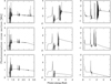 |
Fig. 4 Photoionization cross sections for the 2s22p4 3P2 ground level (left panels), as well as the 2s22p33s 5S2 (middle panels) and 2s22p33s 5P1 (right panels) levels. The results of the present calculation, also reported in Bergemann et al. (2021), are depicted by the top panels, and the results of Nahar (2021) and the OP (Cunto et al. 1993) are presented in the middle and bottom panels, respectively. |
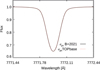 |
Fig. 5 Model line profile for the O I λ7771 transition in the solar photosphere. The line was modeled using the present photoionization cross sections found in Bergemann et al. (2021) (B+2021) and the OP cross sections are taken from TOPbase (Cunto et al. 1993). |
6 Summary and conclusions
We carried out very large calculations of f values and transition probabilities for dipole-allowed lines used in non-LTE analysis of solar photospheric spectra of O and N (Bergemann et al. 2021; Magg et al. 2022). We used various methods and codes for these calculations, namely AUTOSTRUCTURE, R-matrix, GRASP2018, and HFR+CPOL. The convergence of calculated oscillator strength values was evaluated by various criteria including the following: the stability of the numeric values as more configurations are accounted for in the CI expansion; the agreement between values calculated by different gauges; and the agreement among different methods. This allowed us to propose reliable rates with estimated uncertainties. We find satisfactory agreement, within our estimated uncertainties, between our recommended values with those from NIST (Kramida et al. 2021). However, it is seen that the uncertainties stated in the NIST database are overestimated.
We also present the details of R-matrix calculations of O photoionization cross sections that were reported in Bergemann et al. (2021). Our results are more extensive and detailed than previous calculations by other authors. We also quantified the influence of adopted photoionization cross sections on the spectroscopic estimate of the solar O abundance, using the OP cross sections. We confirm that the 3D non-LTE value presented by Bergemann et al. is robust and unaffected by the choice of photoionization data, contrary to the claim made by Nahar (2022).
References
- Asplund, M., Amarsi, A. M., & Grevesse, N. 2021, A&A, 653, A141 [NASA ADS] [CrossRef] [EDP Sciences] [Google Scholar]
- Badnell, N. R. 2011, Comput. Phys. Commun., 182, 1528 [NASA ADS] [CrossRef] [Google Scholar]
- Bensby, T., Feltzing, S., & Oey, M. S. 2014, A&A, 562, A71 [NASA ADS] [CrossRef] [EDP Sciences] [Google Scholar]
- Bergemann, M., Sesar, B., Cohen, J. G., et al. 2018, Nature, 555, 334 [Google Scholar]
- Bergemann, M., Hoppe, R., Semenova, E., et al. 2021, MNRAS, 508, 2236 [NASA ADS] [CrossRef] [Google Scholar]
- Berrington, K. A., Eissner, W. B., & Norrington, P. H. 1995, Comput. Phys. Commun., 92, 290 [NASA ADS] [CrossRef] [Google Scholar]
- Borsa, F., Fossati, L., Koskinen, T., Young, M. E., & Shulyak, D. 2021, Nat. Astron., 6, 226 [Google Scholar]
- Bridges, J. M., & Wiese, W. L. 2010, Phys. Rev. A, 82, 024502 [NASA ADS] [CrossRef] [Google Scholar]
- Civiš, S., Kubelík, P., Ferus, M., et al. 2018, ApJS, 239, 11 [CrossRef] [Google Scholar]
- Collet, R., Magic, Z., & Asplund, M. 2011, J. Phys. Conf. Ser., 328, 012003 [NASA ADS] [CrossRef] [Google Scholar]
- Cowan, R. D. 1981, The Theory of Atomic Structure and Spectra (California: The University of California Press) [Google Scholar]
- Cunto, W., Mendoza, C., Ochsenbein, F., & Zeippen, C. J. 1993, A&A, 275, L5 [NASA ADS] [Google Scholar]
- Froese Fischer, C., Gaigalas, G., Jönsson, P., & Bieroń, J. 2019, Comput. Phys. Commun., 237, 184 [NASA ADS] [CrossRef] [Google Scholar]
- Froese Fischer, C., Godefroid, M., Brage, T., Jönsson, P., & Gaigalas, G. 2016, J. Phys. B Atm. Mol. Phys., 49, 182004 [NASA ADS] [CrossRef] [Google Scholar]
- Grant, I. P. 2007, Relativistic Quantum Theory of Atoms and Molecules (Berlin: Springer), 40 [Google Scholar]
- Grevesse, N., & Sauval, A. J. 1998, Space Sci. Rev., 85, 161 [Google Scholar]
- Gudiksen, B. V., Carlsson, M., Hansteen, V. H., et al. 2011, A&A, 531, A154 [NASA ADS] [CrossRef] [EDP Sciences] [Google Scholar]
- Hibbert, A., Biémont, E., Godefroid, M., & Vaeck, N. 1991a, J. Phys. B Atm. Mol. Phys., 24, 3943 [NASA ADS] [CrossRef] [Google Scholar]
- Hibbert, A., Biémont, E., Godefroid, M., & Vaeck, N. 1991b, A&AS, 88, 505 [NASA ADS] [Google Scholar]
- Johnson, W. R., Kolb, D., & Huang, K. N. 1983, Atm. Data Nucl. Data Tables, 28, 333 [NASA ADS] [CrossRef] [Google Scholar]
- Kramida, A., Ralchenko, Y., Reader, J., & NIST ASD Team 2021, DOI: https://dx.doi.org/10.18434/T4W30F https://www.nist.gov/pml/atomic-spectra-database [Google Scholar]
- Lodders, K. 2019, arXiv e-prints [arXiv:1912.00844] [Google Scholar]
- Magg, E., Bergemann, M., Serenelli, A., et al. 2022, A&A, 661, A140 [NASA ADS] [CrossRef] [EDP Sciences] [Google Scholar]
- Musielok, J., Wiese, W. L., & Veres, G. 1995, Phys. Rev. A, 51, 3588 [CrossRef] [Google Scholar]
- Nahar, S. N. 2021, Atoms, 9, 73 [NASA ADS] [CrossRef] [Google Scholar]
- Nahar, S. N. 2022, MNRAS, 512, L39 [NASA ADS] [CrossRef] [Google Scholar]
- Quinet, P., Palmeri, P., Biémont, E., et al. 1999, MNRAS, 307, 934 [NASA ADS] [CrossRef] [Google Scholar]
- Quinet, P., Palmeri, P., Biémont, E., Li, Z. S., & Svanberg, S. 2002, J. Alloys Compounds, 344, 255 [CrossRef] [Google Scholar]
- Schuler, S. C., Andrews, J. J., Clanzy, V. R., et al. 2021, AJ, 162, 109 [NASA ADS] [CrossRef] [Google Scholar]
- Seaton, M. J. 1987, J. Phys. B Atm. Mol. Phys., 20, 6363 [NASA ADS] [CrossRef] [Google Scholar]
- Serenelli, A. M., Basu, S., Ferguson, J. W., & Asplund, M. 2009, ApJ, 705, L123 [Google Scholar]
- Serenelli, A. M., Haxton, W. C., & Peña-Garay, C. 2011, ApJ, 743, 24 [NASA ADS] [CrossRef] [Google Scholar]
- Tachiev, G. I., & Froese Fischer, C. 2002, A&A, 385, 716 [NASA ADS] [CrossRef] [EDP Sciences] [Google Scholar]
- Tautvaišiene, G., Drazdauskas, A., Bragaglia, A., et al. 2022, A&A, 658, A80 [CrossRef] [EDP Sciences] [Google Scholar]
- Turrini, D., Schisano, E., Fonte, S., et al. 2021, ApJ, 909, 40 [Google Scholar]
- Villante, F. L., & Serenelli, A. 2020, ArXiv e-prints [arXiv:2004.06365] [Google Scholar]
All Tables
Comparison of experimental and predicted ab initio energies in Ryd from our different AUTOSTRUCTURE target expansions for O.
Comparison of experimental and predicted ab initio energies in Ryd from our different AUTOSTRUCTURE target expansions for N.
Comparison of experimental and predicted energies in Ryd from our R-matrix, HFR, and MCDHF calculations for O.
Comparison of experimental and predicted energies in Ryd from our HFR and MCDHF calculations for N.
Comparison of gf values and radiative rates with previously published data for O dipole transitions.
Comparison of gf values and radiative rates with previously published data for N dipole transitions.
All Figures
|
Fig. 1 gf values for the O I λ7771 line. The results of all different model calculations are shown in increasing order of complexity from left to right. The values depicted are AUTOSTRUCTURE length (AUTOSS (L)) and velocity (AUTOSS (V)) gauges as circles and square points, respectively; MCDHF Babushkin (MCDHF (B)) and Coulomb (MCDHF (C)) gauges are shown with diamond and triangular points, respectively; HFR+CPOL is the horizonal long-dashed line; and R-matrix length (R-matrix(L)) and velocity (R-matrix(V)) gauges are shown with dot-dashed lines. The point with error bars at the right end of the plot depicts our recommended gf fvalue for the transitions and its estimated uncertainty. |
| In the text | |
|
Fig. 2 gf values for the N I λ8683 line. The different point types and lines are the same as in Fig. 1. |
| In the text | |
|
Fig. 3 gf values for the N I λ8629 line. The different point types and lines are the same as in Fig. 1. |
| In the text | |
|
Fig. 4 Photoionization cross sections for the 2s22p4 3P2 ground level (left panels), as well as the 2s22p33s 5S2 (middle panels) and 2s22p33s 5P1 (right panels) levels. The results of the present calculation, also reported in Bergemann et al. (2021), are depicted by the top panels, and the results of Nahar (2021) and the OP (Cunto et al. 1993) are presented in the middle and bottom panels, respectively. |
| In the text | |
|
Fig. 5 Model line profile for the O I λ7771 transition in the solar photosphere. The line was modeled using the present photoionization cross sections found in Bergemann et al. (2021) (B+2021) and the OP cross sections are taken from TOPbase (Cunto et al. 1993). |
| In the text | |
Current usage metrics show cumulative count of Article Views (full-text article views including HTML views, PDF and ePub downloads, according to the available data) and Abstracts Views on Vision4Press platform.
Data correspond to usage on the plateform after 2015. The current usage metrics is available 48-96 hours after online publication and is updated daily on week days.
Initial download of the metrics may take a while.