| Issue |
A&A
Volume 665, September 2022
|
|
|---|---|---|
| Article Number | A152 | |
| Number of page(s) | 6 | |
| Section | Stellar atmospheres | |
| DOI | https://doi.org/10.1051/0004-6361/202243784 | |
| Published online | 23 September 2022 | |
Radio detection of chemically peculiar stars with LOFAR
1
Space Radio-Diagnostics Research Centre, University of Warmia and Mazury,
ul.Oczapowskiego 2,
10-719
Olsztyn, Poland
e-mail: This email address is being protected from spambots. You need JavaScript enabled to view it.
2
INAF – Osservatorio Astrofisico di Catania,
Via S. Sofia 78,
95123
Catania, Italy
3
ASTRON, Netherlands Institute for Radio Astronomy,
Oude Hoogeveensedijk 4,
Dwingeloo
7991 PD, The Netherlands
4
Department of Astrophysics/IMAPP, Radboud University,
PO Box 9010,
6500 GL
Nijmegen, The Netherlands
5
Leiden Observatory, Leiden University,
PO Box 9513,
2300 RA
Leiden, The Netherlands
6
Department of Physics and Astronomy, The Open University,
Walton Hall,
Milton Keynes
MK7 6AA, UK
7
STFC Rutherford Appleton Laboratory,
Chilton, Didcot, Oxfordshire
OX11 0QX, UK
Received:
13
April
2022
Accepted:
2
July
2022
Abstract
Context. Chemically peculiar stars are upper main sequence stars that show anomalies in their optical spectra. These anomalies suggest peculiar chemical abundances of certain elements. Some chemically peculiar stars possess strong magnetic fields. Electrons originating from the ionising stellar wind travel in the magnetosphere of the star and become the source of non-thermal radio and X-ray emission. Several chemically peculiar radio stars have been detected at GHz frequencies.
Aims. We used the Low-Frequency Array (LOFAR) to search for radio emission from chemically peculiar stars to constrain their emission in the frequency band 120–168 MHz. We aimed to use LOFAR observations to test the models for radio emission of chemically peculiar stars.
Methods. We performed a targeted search of known chemically peculiar stars in the fields of the LOFAR Two Metre Survey (LoTSS) Data Release 2 in Stokes I and V. We matched positions of radio sources in the LoTSS-DR2 catalogue with positions of chemically peculiar stars.
Results. We report non-thermal emission at 120–168 MHz from two chemically peculiar stars in Stokes I, BP Boo, and α2 CVn. The ensuing incidence rate at these frequencies is significantly lower than for higher frequencies. This results from the turnover at low frequencies which was predicted from the theory of radio emission from chemically peculiar stars. BP Boo is detected for the first time at radio wavelengths, while α2 CVn had already been detected at higher frequencies. The upper limit of V/I indicates a level of circular polarisation significantly below 60%. We combined data obtained at different frequencies to derive the radio spectrum of α2 CVn. The spectrum is nearly flat beyond turnover at low frequencies. We modelled radio emission for a large magnetosphere and small local magnetic field strength. The amplitude of variation in radio emission with the rotational phase of the system decreases at low frequencies.
Key words: stars: chemically peculiar / stars: early-type / radio continuum: stars
© M. Hajduk et al. 2022
 Open Access article, published by EDP Sciences, under the terms of the Creative Commons Attribution License (https://creativecommons.org/licenses/by/4.0), which permits unrestricted use, distribution, and reproduction in any medium, provided the original work is properly cited.
This article is published in open access under the Subscribe-to-Open model. This email address is being protected from spambots. You need JavaScript enabled to view it. to support open access publication.
1 Introduction
Chemically peculiar (CP) stars are main sequence stars with spectral types in the range of B8–A7. Their optical spectra show abnormally strong or weak lines of certain elements, such as Si, Sr, Cr, and rare earths (Morgan 1933). Their rotation periods range from 0.5 to thousands of days (Netopil et al. 2017). The first CP star, α2 Canum Venaticorum, was discovered by Maury & Pickering (1897).
Preston (1974) presents a classification of CP stars based on their optical spectra. CP1 stars are metallic-line, non-magnetic Am stars. CP2 stars are magnetic Ap stars, where p indicates peculiarity of their spectra. CP3 stars are stars enhanced in mercury and manganese, while CP4 stars are He-weak (He-W). In addition, He-strong (He-S) stars and λ Boo stars form separate groups of CP stars (Venn & Lambert 1990).
Strong, globally organised magnetic fields that are mainly dipolar, with strength ≳300 G (Shultz et al. 2019), and that are inclined to the rotational axis (oblique rotator model: ORM, Babcock 1949; Stibbs 1950) can account for some properties of CP stars (Aurière et al. 2007; Sikora et al. 2019b); these properties can lead to the development of surface abundance inhomogeneities (Michaud et al. 1981).
In some cases, UV spectral features were observed that were ascribed to the presence of ionised circumstellar material (Shore & Brown 1990). The material was likely lost by the radiatively driven stellar wind. The presence of plasma in the presence of a magnetic field may be a suitable condition for non-thermal radio emission generation.
Drake et al. (1987) first discovered non-thermal radio emission from chemically peculiar stars with the Very Large Array (VLA). The initial sample used by these latter authors was later complemented by Linsky et al. (1992). These authors detected 12 helium-weak and 3 helium-strong stars, and no classical (SrCrEu-type) Ap stars in the observed sample of 61 objects. Their average detection rate was 23% at 5 GHz with a sensitivity of the order of 0.1 mJy. Linsky et al. (1992) calculated that He-W stars are on average 20 times less luminous in radio than He-S stars, and concluded that radio luminosity of CP stars L6 correlates with magnetic field strength Brms and effective temperature of the star.
Leone et al. (1994) estimated the incidence ratio for radio-emitting CP stars to 31% for He-S stars, 26% for He-W stars, 23% for Si stars, and 0% for cool Ap stars. The most recent compilation of radio-detected early-type stars was presented by Shultz et al. (2022). These authors concluded that gyro-synchrotron emission is observed in stars that are young, strongly magnetic (log(Bd/G) ≈ 3.7), and rapidly rotating (Prot ≲ 5 days).
Leto et al. (2021) calculated radio spectra from CP stars over a broad range of frequencies. Most of the non-thermal radio emission originates from the regions at higher magnetic latitudes. The electrons accelerated up to relativistic energies in the equatorial magneto-disc produce radio emission by the incoherent gyro-synchrotron mechanism in the middle magnetosphere. The low-frequency side of the radio spectrum traces the radio emission arising from the furthest regions of the middle magnetosphere. The turnover frequency of the gyro-synchrotron radio spectrum is proportional to the local magnetic field strength (Dulk & Marsh 1982).
The chemically peculiar magnetic stars are also a source of coherent radio emission amplified by the electron cyclotron maser emission (ECME) mechanism. The ECME mainly amplifies the radio frequencies at the first few harmonics of the local gyro-frequency of a specific magneto-ionic mode. This kind of coherent emission mechanism produces amplified radiation constrained within a strongly anisotropic beam pattern. In the case of stars, the ECME is usually driven by the loss-cone unstable electron energy distribution. The first detection of ECME was reported by Trigilio et al. (2000), who discovered nearly 100% circularly polarised emission from the ApSi CP star CU Vir at 1.4 GHz, later confirmed by Das & Chandra (2021). ρ OpHC shows 60% polarised emission at 1.6 GHz, decreasing with frequency (Leto et al. 2020a). Das & Chandra (2021) discovered eight stars showing similar properties of radio emission using the Giant Metrewave Radio telescope at the frequency range 0.6−0.8 GHz. The ECME mechanism has been proposed for these objects (Trigilio et al. 2011). The emission occurs at the magnetic null phase of the system. Das et al. (2022) discovered more examples of main sequence radio-pulse emitters, and concluded that at least 32% of the magnetic hot stars exhibit periodic radio pulses produced via electron cyclotron maser emission.
The dipole-dominated magnetospheres of the CP stars are also a site of X-ray emission. X-rays are produced within the magnetopheric region where the magnetic field lines are closed and plasma cannot escape. This region is named the “inner-magnetosphere” The radiatively driven, ionised stellar wind co-rotates with the star in the inner magnetosphere. The wind components originating from the two hemispheres collide at the magnetic equator, forming a shocked disc where thermal X-rays are produced. This scenario is summarised within the magnetic confined wind shock (MCWS) model (Babel & Montmerle 1997).
The phenomena observed in the radio regime are the consequence of the interaction between the plasma and the magnetic fields surrounding the star. The CP stars that are radio sources likely host large-scale co-rotating magnetospheres. At large distances, centrifugal breakout (CBO) events continuously occur, providing acceleration of electrons up to relativistic energies (Owocki et al. 2022), which are responsible for the observed radio emission.
2 Radio observations
The LOFAR Two Metre Survey (LoTSS) is an ongoing northern sky survey in the frequency range of 120–168 MHz (Shimwell et al. 2022). LoTSS-DR2 observed 27% of the northern hemisphere with a point-source sensitivity of better than 100 µJy and an angular resolution of 6″. The sensitivity and angular resolution are orders of magnitude better than for previous surveys in this frequency range. Most of the pointings were observed for 8 h. Single pointings were then mosaiced to create final maps.
We performed a targeted search for chemically peculiar stars using positional matching. We corrected the positions for the proper motions using Gaia Collaboration (2021). We used a catalogue by Renson & Manfroid (2009). The fields of LoTSS-DR2 contain 462 stars from Renson & Manfroid (2009). Out these, 136 stars are marked as “doubtful nature”, and 11 are marked “improperly considered Ap or Am”. We discarded Am and HgMn stars, which are not expected to produce radio emission. This left 61 Ap stars, 3 He-W stars, and 1 He-S star. Leone et al. (1994) detected 20 out of the 84 surveyed CP stars (excluding Am stars) with the VLA, while we detected 2 out of 65 stars with LOFAR. The odds ratio is 8 (a range of 1.7–34 with the confidence level of 95%).
We searched only for radio emission originating from Ap stars. Non-magnetic Am stars are not expected to show radio emission; when included, they would increase the chance of a false-positive.
Two Ap stars have counterparts in the LoTSS-DR2 catalogue with a separation <1 arcsec. These sources are α2 CVn with a separation of 0.7 arcsec and BP Boo with a separation of 0.4 arcsec. For all the other sources, separations between the optical and radio source are >7 arcsec. The astrometric precision (one σ) of LoTSS is about 0.5 arcsec for sources detected with S/N of about 5, similar to the two identified sources (Shimwell et al. 2022).
False-positives would dominate a blind search of stars (Callingham et al. 2019). However, the chance of false positive can be reduced in a targeted search for stars. We cross-correlated LoTSS-DR2 with a small sample of fewer than 100 stars. The radio source density of 770 sources per square degree indicates that the probability of false positive is less than 1% in this case. Neither of the detected sources is resolved. α2 CVn and BP Boo are relatively nearby (they belong to the 20% of stars with the largest parallaxes in the studied sample of CP stars). This further increases the chance that these are not false positives.
If we restrict our sample to the “well-known” sample of Ap or He stars defined by Renson & Manfroid (2009), then the incidence rate for 2 out of 28 is 0.4−33% with a 0.99 confidence level (Gehrels 1986). If we take all the Ap or He stars by Renson & Manfroid (2009) into account, then the incidence rate would be in the range of 0.2−14% for the same confidence level.
α2 CVn was observed on eight different dates. The separation between the position of the star and the phase centre was different on each date. Each observation covered time spanning approximately 6% of the rotational phase of the system. The star was detected only in one image and in the final, mosaiced image. α2CVn was detected at the level of 410 ± 120 µJy at Stokes I. We did not detect Stokes V to a one-sigma upper limit of 80 µJy. One sigma upper limit for circular polarisation is about 20%.
The observation carried out on 2017 Feb 23, when the star was detected, has the best S/N and its phase centre is closest to the star (Table 1). The star was further away from the phase centre on the other dates and the quality of the maps is much poorer. The star would not be bright enough to be detected on the other dates, assuming that the flux is constant. Therefore, no firm conclusions can be made about the source variability.
BP Boo is detected at the level of 320 ± 90 µJy. Its one sigma upper limit for Stokes V is 50 µJy, and so the one-sigma limit for circular polarisation is about 20%, similar to α2 CVn. It has also been detected in only one out of eight pointings, the one in which the star is closest to the phase centre (Table 2). Each observation covered time spanning about 25% of the rotational phase of the system.
The remaining stars have not been detected. These include 36 Lyn, which had been previously detected by Drake et al. (2006) at the level of 0.45 mJy at 8 GHz. The upper (one sigma) limit for this star at 120–168 MHz is 0.06 mJy.
Dates, UT, a separation between the star and the phase centre, root mean square (rms) measured on the map, and rotational phase of the star corresponding to the middle of the observation run for α2 CVn.
Dates, UT, separation between the star and the phase centre, rms measured on the map and rotational phase of the star corresponding to the middle of the observation run for BP Boo.
3 Discussion
We used the distances to α2 CVn and BP Boo from Gaia DR3 parallaxes (Gaia Collaboration 2021) to calculate their radio luminosities. The derived luminosities are presented in Table 3 and shown in Fig. 1. One group of stars has lower upper limits for radio luminosities than α2 CVn and BP Boo; however, they are of later spectral types or more evolved than the detected stars. Their expected radio emission would be much lower (Shultz et al. 2022).
The radio flux densities, stellar parameters, luminosities, and brightness temperatures of the detected objects are listed in Table 3. For the computation of brightness temperatures, we assumed that the size of the emission is equal to one stellar radius.
The two CP stars detected with LOFAR represent the Ap type. Our survey included one He-S star and three He-W stars, all undetected. Two of them have upper limits lower than the luminosity for BP Boo. However, with the current precision and statistics, it is difficult to state whether He-S/He-W stars have higher luminosities than Ap stars at MHz frequencies, which is similar to the findings of Linsky et al. (19920) at GHz frequencies.
α2 CVn was identified at the level of 850 in the FIRST survey (Helfand et al. 1999) at 1.4 GHz, which is slightly higher than our detection in LoTSS DR2. It has also been observed by Drake et al. (2006) at 8 GHz, and at 3 GHz by Leto et al. (2021). The radio spectrum is presented in Fig. 2 and Table 4. The spectrum is relatively flat and extends down to 144 MHz, assuming that temporal variability is not significant.
BP Boo has not yet been detected at higher frequencies and was not detected in the FIRST survey (the upper limit of 1 mJy). This suggests that its radio spectrum is relatively flat.
We derived brightness temperatures of the order of 1010 – 1011 K for the detected stars assuming the size of the emission to correspond to one stellar radius. Such a high brightness temperature suggests non-thermal emission. However, low-frequency radio emission may originate from the distant regions of the magnetosphere, close to the Alfvén boundary, and therefore the computed brightness temperatures may be overestimated. On the other hand, the computed brightness temperature would be underestimated if the emission was directional.
Gyro-synchrotron radio spectra peak at the turnover frequency, which is proportional to the local magnetic field strength (Dulk & Marsh 1982). For α2 CVn, the turnover frequency is at about 3 GHz. This is similar to turnover frequencies for other CP stars (Leto et al. 2021).
Previous studies suggest the existence of both low- and high-frequency cutoffs in radio spectra of CP stars. Leto et al. (2021) present a model in which radio spectra of most CP stars drop rapidly towards lower frequencies. In this model, low-frequency emission is produced external to the central magnetosphere, in the regions which are not crossed by relativistic electrons.
Low-frequency detections of α2 CVn and BP Boo suggest that, at least in some cases, the drop in low-frequency radio emission is not as steep as previously assumed. This suggests that a significant amount of emission arises at a large distance from the star, where the magnetic field is relatively weak.
α2 CVn is a star with one of the longest rotational periods detected in the sample of radio-emitting stars (Shultz et al. 2022). α2 CVn has a rotational period of about 5.47 day−1. BP Boo has a much shorter period of 1.29 day−1 (Sikora et al. 2019b).
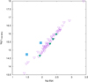 |
Fig. 1 Detections and non-detections of CP stars with LOFAR. Inversed triangles mark non-detections, squares mark detections of α2 CVn and BP Boo. The filled inversed triangles mark the upper limit for the three He-W stars and a He-S star. |
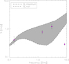 |
Fig. 2 Radio spectrum of α2 CVn. We used radio flux densities collected in different epochs. The grey-shaded region shows the range of the simulated flux densities. |
Parameters for the detected stars.
Radio detections of α2 CVn.
4 Radio emission model for α2 CVn
We calculated the radio spectrum of α2 CVn in the range 0.1 – 10 GHz. For the calculation of the radio flux for incoherent gyro-synchrotron emission, we used the 3D model developed by Trigilio et al. (2004) and Leto et al. (2006). The model samples the space surrounding the star using a 3D Cartesian grid, where all the physical parameters needed for the calculation of the emission and absorption coefficients for the gyro-synchrotron emission mechanism (Ramaty 1969; Klein 1987) are estimated. The radiative transfer equation was integrated along the ray paths parallel to the line of sight. The frequency-dependent absorption effects due to the ambient thermal plasma trapped within the stellar magnetosphere were also taken into account. Once assigned the stellar geometry, the total flux radiated by the stellar magnetosphere was calculated as a function of the stellar rotational phase (for additional details, see Trigilio et al. 2004 and Leto et al. 2006). In the case of α2 CVn, the calculations have been made at two stellar rotational phases, corresponding to the null and to the magnetic field maximum. The null coincides with the stellar orientation that makes the dipole axis perpendicular to the line of sight. The ORM geometry of α2 CVn (see Table5) makes the northern hemisphere more visible, and the maximum of the effective magnetic field is positive and coincides with the stellar orientation, which makes the north magnetic pole more visible. Conversely, the negative extremum has a lower absolute strength and is related to the better visibility of the south magnetic pole, and the calculated radio emission is consequently lower.
The model parameters explored are: (i) the L-shell parameter (unit stellar radii), that is the distance where the dipole magnetic field line crosses the magnetic equator. This parameter then quantifies the equatorial size of the stellar magnetosphere; and (ii) nrel × l (unit cm−2), that is the column density of the relativistic electrons at the distance from the stellar centre L, where nrel is the density of the non-thermal electrons, which is constant within the dipole magnetic shell where the relativistic electrons freely propagate, l is the thickness of this magnetic shell at the distance L. The two parameters nrel and l are degenerate parameters, which is why we report their product only.
The parameter L was varied in the range 15–25 R* (with the step of 1 R*). The parameter nrel × l was varied in the range 1013.5−1014.5 cm−2 (with a step of 0.1 in log).
We followed the same modelling approach described in Leto et al. (2021). As discussed in that paper, the other model parameters were left fixed and are: thermal electron density at the stellar surface, n0 = 3 × 109cm−3; and the spectral index of the energy distribution (power-law) of the non-thermal electrons, δ = 2.5. The other stellar parameters needed for the radio emission calculations are listed in Table5.
The adopted sampling of the Cartesian grid is variable as a function of radial distance. At distances larger than 12 R*, a rough sampling was adopted, corresponding to a sampling step of 1 R*. At intermediate distances in the range 6–12 R*, a sampling step of 0.5 R* was adopted. Approaching the star, at a distance of less than 6 R*, the thinner sampling of 0.25 R* was adopted.
Among the calculated spectra, the one that is most in accordance with the multifrequency available radio measurements was performed using L ≈ 20 R* and nrel × l ≈ 1013.9cm−2. The non-thermal acceleration equatorial regions are located on average at 20 R* from the centre of the star. The local magnetic field strength is about 0.2 G. The local density of the thermal electrons is 1.5 × 108 cm−3, calculated using the linear spatial dependence. This is because, following the magnetically confined wind-shock model (Babel & Montmerle 1997), the thermal plasma density trapped by the closed magnetic field lines linearly decreases as a function of the radial distance, whereas the temperature linearly increases. This implies that the plasma pressure is constant within the magnetospheric region where the thermal plasma is trapped by the magnetic field strength. Close to the non-thermal acceleration regions, which were estimated to be located at about 20 stellar radii, the magnitude of the local energy density of the magnetic field (B2/8π, B in Gauss) of 10−3 erg/cm−3 is similar to the thermal plasma energy density. Further, the centrifugal force provided by the stellar rotation makes these distant magnetospheric regions unstable and no longer able to confine the ambient plasma. This supports the scenario where the relativistic electrons are provided by continuous breakout events (Owocki et al. 2022).
The oblique rotator model geometry of α2 CVn gives rise to large rotational variability in the radio emission, mainly at the intermediate and higher frequencies. The lower simulated radio frequencies are instead less affected by rotational variability. Figure 2 presents the range of the simulated flux densities superimposed on the observed radio spectrum.
The lower level of the simulated emission is related to the stellar orientation corresponding to the magnetic null. The upper envelope of the grey area corresponds to the radio emission arising from α2 CVn when the star shows the north magnetic pole.
Excluding the measurement at the highest frequency, the other three are well within the expected radio emission range. As discussed at length by Leto et al. (2021), when approaching the stellar surface, a possible high-frequency cutoff or model inability to correctly estimate the radio emission makes the comparison between simulations and observations unreliable at the high-frequency range. We note that the high-frequency side of the radio spectrum is not absolute. The radio frequency when the discrepancy starts is a function of the parameters of the stellar magnetosphere. The comparison between the measured and calculated radio spectra of α2 CVn agrees with the general results summarised by the low, intermediate, and high-frequency behaviours discussed by Leto et al. (2021). In particular, the radio emission at 144 MHz from α2 CVn mainly originates from regions outward from the inner magnetosphere, where the thermal plasma is trapped. Therefore, the radio emission arising from the magnetospheric regions located in front of the observer travels almost in a vacuum.
We cannot exclude the possibility that radio emission is generated via ECME. The computed brightness temperature would be much higher for directional emission than 7.5 × 10¹⁰ K which was computed assuming an emitting region similar in size to the stellar radius (Table 3).
For ECME, the observed circular polarisation would depend on the propagation effects (Leto et al. 2016; Das et al. 2020), and therefore the low circular polarisation observed for α2 CVn cannot exclude this mechanism. To verify the emission mechanism, one could fold the radio light curve with the rotational period. ECME is seen at a rotational phase corresponding to the magnetic null phase (Trigilio et al. 2000; Das et al. 2022). If the flux was found to not vary significantly with rotational phase, this would suggest emission from the outer magnetosphere.
The value of the longitudinal magnetic field is approximately 0 for the phase of 0.7 and 0.3 in α2 CVn (Kochukhov et al. 2002). The star was detected in only one pointing with LOFAR, corresponding to the rotational phase of 0.7. However, the other pointings had much lower S/N and would not be detected unless the flux density was significantly higher than 0.41 mJy observed at phase 0.7.
Very Large Array Sky Survey (VLASS) observed the star at 2–4 GHz near rotational phases of 0.3 and 0.8 (Table 4). The phase of 0.3 corresponds to the null phase, and the phase of 0.8 does not. The observed variability is consistent with the rotational modulation of incoherent emission in the range of 1–5 GHz predicted by the ORM scenario. Otherwise, the ECME would show much larger amplitude variations with phase.
The magnetic field configuration in BP Boo is unknown. Assuming that the star has a roughly constant flux density of 0.32 mJy, it would not be detected in any other pointing except the closest one. Therefore, no conclusions can be drawn.
Adopted parameters for the model of α2 CVn: distance, radius, effective temperature, the dipole field strengths, rotation axis inclination, and dipole axis obliquity.
5 Discussion and conclusions
We detected two chemically peculiar stars in LoTSS-DR2. The sensitivity of the LoTSS survey of 0.1 mJy is comparable to the sensitivity of the targeted surveys carried out with the VLA. However, CP stars are intrinsically weaker at 144MHz than at GHz frequencies, which makes the incidence rate of chemically peculiar stars at 144MHz much lower than at GHz frequencies. A more complete sample of 144 MHz detections of CP stars will allow us to model their radio spectra for a much broader range of frequencies than has been achieved so far. Low-frequency emission samples the most distant regions of the stellar magneto-sphere. α2 CVn has the lowest local magnetic field strength and the most extended equatorial size of magnetosphere compared to the sample analysed by Leto et al. (2021). The stellar rotation period of α2 CVn is significantly larger than the periods of the stars whose radio spectra were modelled, which implies that the Keplerian co-rotation radius (RK) of α2 CVn is also larger. This radius is about 7.6 R*, which was calculated using the relation  , where G is the gravitational constant and ω the angular velocity (Leto et al. 2020b), which is much larger than the Keplerian radii (typically about a couple of stellar radii) of that sample (Shultz et al. 2020). In any case, the modelling of the low-frequency side of the radio spectrum of α2 CVn allowed us to constrain the distance where the magnetically supported co-rotation breaks. These regions are located well beyond the RK size, which is a clear indication of the existence of a centrifugal magnetosphere where the centrifugal force supports the co-rotating material against the gravitational force (Petit et al. 2013). Therefore, the detection of its radio emission at 144 MHz is further confirmation of the expected spectral behaviour of the incoherent gyro-synchrotron emission from the large-scale co-rotating magnetospheres surrounding early-type magnetic stars.
Acknowledgements
M.H. acknowledges the MSHE for granting funds for the Polish contribution to the International LOFAR Telescope (MSHE decision no. DIR/WK/2016/2017/05-1) and for maintenance of the LOFAR PL-612 Baldy (MSHE decision no. 59/E-383/SPUB/SP/2019.1) and the Polish National Agency for Academic Exchange (NAWA) within the Bekker programme under grant no. PPN/BEK/2019/1/00431. MHav acknowledges funding from the European Research Council (ERC) under the European Union’s Horizon 2020 research and innovation programme (grant agreement no. 772663).
References
- Aurière, M., Wade, G. A., Silvester, J., et al. 2007, A&A, 475, 1053 [NASA ADS] [CrossRef] [EDP Sciences] [Google Scholar]
- Babcock, H. W. 1949, The Observatory, 69, 191 [NASA ADS] [Google Scholar]
- Babel, J., & Montmerle, T. 1997, A&A, 323, 121 [NASA ADS] [Google Scholar]
- Callingham, J. R., Vedantham, H. K., Pope, B. J. S., Shimwell, T. W., & LoTSS Team. 2019, RNAAS, 3, 37 [NASA ADS] [Google Scholar]
- Das, B., & Chandra, P. 2021, ApJ, 921, 9 [NASA ADS] [CrossRef] [Google Scholar]
- Das, B., Mondal, S., & Chandra, P. 2020, ApJ, 900, 156 [NASA ADS] [CrossRef] [Google Scholar]
- Das, B., Chandra, P., Shultz, M. E., et al. 2022, ApJ, 925, 125 [NASA ADS] [CrossRef] [Google Scholar]
- Drake, S. A., Abbott, D. C., Bastian, T. S., et al. 1987, ApJ, 322, 902 [NASA ADS] [CrossRef] [Google Scholar]
- Drake, S. A., Wade, G. A., & Linsky, J. L. 2006, in ESA Special Publication, The X-ray Universe 2005, ed. A. Wilson, 604, 73 [Google Scholar]
- Dulk, G. A., & Marsh, K. A. 1982, ApJ, 259, 350 [NASA ADS] [CrossRef] [Google Scholar]
- Gaia Collaboration (Brown, A. G. A., et al.) 2021, A&A, 649, A1 [NASA ADS] [CrossRef] [EDP Sciences] [Google Scholar]
- Gehrels, N. 1986, ApJ, 303, 336 [Google Scholar]
- Helfand, D. J., Schnee, S., Becker, R. H., White, R. L., & McMahon, R. G. 1999, AJ, 117, 1568 [Google Scholar]
- Klein, K. L. 1987, A&A, 183, 341 [NASA ADS] [Google Scholar]
- Kochukhov, O., Piskunov, N., Ilyin, I., Ilyina, S., & Tuominen, I. 2002, A&A, 389, 420 [NASA ADS] [CrossRef] [EDP Sciences] [Google Scholar]
- Leone, F., Trigilio, C., & Umana, G. 1994, A&A, 283, 908 [NASA ADS] [Google Scholar]
- Leto, P., Trigilio, C., Buemi, C. S., Umana, G., & Leone, F. 2006, A&A, 458, 831 [NASA ADS] [CrossRef] [EDP Sciences] [Google Scholar]
- Leto, P., Trigilio, C., Buemi, C. S., et al. 2016, MNRAS, 459, 1159 [NASA ADS] [CrossRef] [Google Scholar]
- Leto, P., Trigilio, C., Buemi, C. S., et al. 2020a, MNRAS, 499, L72 [CrossRef] [Google Scholar]
- Leto, P., Trigilio, C., Leone, F., et al. 2020b, MNRAS, 493, 4657 [Google Scholar]
- Leto, P., Trigilio, C., Krtička, J., et al. 2021, MNRAS, 507, 1979 [NASA ADS] [CrossRef] [Google Scholar]
- Linsky, J. L., Drake, S. A., & Bastian, T. S. 1992, ApJ, 393, 341 [Google Scholar]
- Maury, A. C., & Pickering, E. C. 1897, Ann. Harvard College Observ., 28, 1 [NASA ADS] [Google Scholar]
- Michaud, G., Megessier, C., & Charland, Y. 1981, A&A, 103, 244 [NASA ADS] [Google Scholar]
- Morgan, W. W. 1933, ApJ, 77, 330 [NASA ADS] [CrossRef] [Google Scholar]
- Netopil, M., Paunzen, E., Hümmerich, S., & Bernhard, K. 2017, MNRAS, 468, 2745 [NASA ADS] [CrossRef] [Google Scholar]
- Owocki, S. P., Shultz, M. E., ud-Doula, A., et al. 2022, MNRAS, 513, 1449 [NASA ADS] [CrossRef] [Google Scholar]
- Petit, V., Owocki, S. P., Wade, G. A., et al. 2013, MNRAS, 429, 398 [NASA ADS] [CrossRef] [Google Scholar]
- Preston, G. W. 1974, ARA&A, 12, 257 [Google Scholar]
- Ramaty, R. 1969, ApJ, 158, 753 [CrossRef] [Google Scholar]
- Renson, P., & Manfroid, J. 2009, A&A, 498, 961 [NASA ADS] [CrossRef] [EDP Sciences] [Google Scholar]
- Shimwell, T. W., Hardcastle, M. J., Tasse, C., et al. 2022, A&A, 659, A1 [NASA ADS] [CrossRef] [EDP Sciences] [Google Scholar]
- Shore, S. N., & Brown, D. N. 1990, ApJ, 365, 665 [NASA ADS] [CrossRef] [Google Scholar]
- Shultz, M. E., Wade, G. A., Rivinius, T., et al. 2019, MNRAS, 490, 274 [NASA ADS] [CrossRef] [Google Scholar]
- Shultz, M. E., Owocki, S., Rivinius, T., et al. 2020, MNRAS, 499, 5379 [NASA ADS] [CrossRef] [Google Scholar]
- Shultz, M. E., Owocki, S. P., ud-Doula, A., et al. 2022, MNRAS, 513, 1429 [NASA ADS] [CrossRef] [Google Scholar]
- Sikora, J., Wade, G. A., Power, J., & Neiner, C. 2019a, MNRAS, 483, 2300 [NASA ADS] [CrossRef] [Google Scholar]
- Sikora, J., Wade, G. A., Power, J., & Neiner, C. 2019b, MNRAS, 483, 3127 [NASA ADS] [CrossRef] [Google Scholar]
- Stibbs, D. W. N. 1950, MNRAS, 110, 395 [Google Scholar]
- Trigilio, C., Leto, P., Leone, F., Umana, G., & Buemi, C. 2000, A&A, 362, 281 [Google Scholar]
- Trigilio, C., Leto, P., Umana, G., Leone, F., & Buemi, C. S. 2004, A&A, 418, 593 [NASA ADS] [CrossRef] [EDP Sciences] [Google Scholar]
- Trigilio, C., Leto, P., Umana, G., Buemi, C. S., & Leone, F. 2011, ApJ, 739, L10 [NASA ADS] [CrossRef] [Google Scholar]
- Venn, K. A., & Lambert, D. L. 1990, ApJ, 363, 234 [Google Scholar]
All Tables
Dates, UT, a separation between the star and the phase centre, root mean square (rms) measured on the map, and rotational phase of the star corresponding to the middle of the observation run for α2 CVn.
Dates, UT, separation between the star and the phase centre, rms measured on the map and rotational phase of the star corresponding to the middle of the observation run for BP Boo.
Adopted parameters for the model of α2 CVn: distance, radius, effective temperature, the dipole field strengths, rotation axis inclination, and dipole axis obliquity.
All Figures
|
Fig. 1 Detections and non-detections of CP stars with LOFAR. Inversed triangles mark non-detections, squares mark detections of α2 CVn and BP Boo. The filled inversed triangles mark the upper limit for the three He-W stars and a He-S star. |
| In the text | |
|
Fig. 2 Radio spectrum of α2 CVn. We used radio flux densities collected in different epochs. The grey-shaded region shows the range of the simulated flux densities. |
| In the text | |
Current usage metrics show cumulative count of Article Views (full-text article views including HTML views, PDF and ePub downloads, according to the available data) and Abstracts Views on Vision4Press platform.
Data correspond to usage on the plateform after 2015. The current usage metrics is available 48-96 hours after online publication and is updated daily on week days.
Initial download of the metrics may take a while.