| Issue |
A&A
Volume 664, August 2022
|
|
|---|---|---|
| Article Number | A10 | |
| Number of page(s) | 6 | |
| Section | Stellar structure and evolution | |
| DOI | https://doi.org/10.1051/0004-6361/202243486 | |
| Published online | 03 August 2022 | |
Magnetic effect on equilibrium tides and its influence on the orbital evolution of binary systems
Department of Astronomy, Beijing Normal University, Beijing, PR China
e-mail: This email address is being protected from spambots. You need JavaScript enabled to view it.
Received:
6
March
2022
Accepted:
17
May
2022
Abstract
In the standard theory of equilibrium tides, hydrodynamic turbulence is considered. In this paper we study the effect of magnetic fields on equilibrium tides. We find that the turbulent Ohmic dissipation associated with a tidal flow is much stronger than the turbulent viscous dissipation such that a magnetic field can greatly speed up the tidal evolution of a binary system. We then apply the theory to three binary systems: the orbital migration of 51 Pegasi b, the orbital decay of WASP-12b, and the circularization of close binary stars. Theoretical predictions are in good agreement with observations, which cannot be clearly interpreted with hydrodynamic equilibrium tides.
Key words: magnetic fields / turbulence / planet-star interactions / binaries: close
© X. Wei 2022
 Open Access article, published by EDP Sciences, under the terms of the Creative Commons Attribution License (https://creativecommons.org/licenses/by/4.0), which permits unrestricted use, distribution, and reproduction in any medium, provided the original work is properly cited.
This article is published in open access under the Subscribe-to-Open model. This email address is being protected from spambots. You need JavaScript enabled to view it. to support open access publication.
1. Motivation
Tides play a key role in the orbital evolution of a binary system, for example planet–satellite, star–planet, binary stars, and a compact object and its companion. The body on which a tide is exerted is called the primary and the body that raises a tide is called the secondary. Tidal force is the gravitational perturbation, which is inversely proportional to the cube of the orbital semimajor axis. A tide can be decomposed into two parts; one is the equilibrium tide, namely a large-scale deformation due to the hydrostatic balance between tidal potential and pressure perturbation, and the other is the dynamical tide, namely fluid waves (gravity waves and inertial waves) excited by tidal force. Equilibrium tides dissipate through turbulence in the convection zone, and the dynamical tides dissipate either through radiative cooling in the radiation zone (gravity wave) or through viscous shears in the convection zone (inertial wave).
The study of tides has a long history, dating back to Newton and Laplace. In the 1950s pioneering work on tidal theory began, and we started to understand the orbital evolution of the satellites in the Solar System (Jeffreys 1961; Goldreich 1963; Goldreich & Soter 1966) and that of the close binary stars in open clusters (Kopal 1959; Zahn 1975, 1977, 1989; Goldreich & Nicholson 1977, 1989; Hut 1981; Savonije & Papaloizou 1983). Since the 1990s with the detection of exoplanets, especially hot Jupiters (exoplanets close to their host stars with orbital periods of several days), the theory and application of equilibrium tides were greatly developed (Lin et al. 1996; Goodman & Oh 1997; Penev et al. 2009; Barker 2020; Terquem 2021). However, the standard theory of equilibrium tides cannot provide sufficient tidal dissipation for the orbital evolution of either star–planet systems or binary star systems. Researchers then turned to dynamical tides (Lai 1997; Goodman & Dickson 1998; Witte & Savonije 2002; Ogilvie & Lin 2004; Wu 2005; Goodman & Lackner 2009; Fuller 2014) and the nonlinear resonance locking of dynamical tides (Weinberg et al. 2012; Zanazzi & Wu 2021).
On the other hand, magnetic fields are ubiquitous in the Universe. In all the models mentioned above the magnetic effect on tides is not involved. In Wei (2016, 2018), and Lin & Ogilvie (2018) the magnetic effect on dynamical tides was considered and it was found that magnetic fields can greatly enhance tidal dissipation. In this paper we consider the magnetic effect on equilibrium tides. We find that magnetic fields can induce much stronger tidal dissipation, and thus a very significant effect on the orbital evolution of binary systems. In Sect. 2 we formulate the expressions of tidal dissipation and torques arising from hydrodynamical and magnetic turbulence. In Sect. 3 we apply our model to interpret the observations of the three binary systems. In Sect. 4 a brief summary is given.
2. Two tidal dissipations and torques
We consider the major quadrupolar component of tidal potential resulting from orbital motion at frequency ωo relative to the primary rotation at frequency ωs, namely an asynchronized tide. The tidal torque Γ exerted on an orbit is related to tidal dissipation D via Γ = −D/(ωo − ωs). Either hydrodynamic or magnetic turbulence can lead to tidal torque, and the only difference lies in dissipation D, whether it is viscous dissipation Dh or Ohmic dissipation Dm. Next we find Dh and Dm. We adopt the conventional notations: primary mass M, secondary mass m, primary radius R, and orbital semimajor axis a.
For hydrodynamic turbulence in the convection zone of a primary, viscous dissipation Dh associated with the large-scale sheared tidal flow u is
 (1)
(1)
where ρ is density, νt turbulent viscosity, d thickness, and V volume of the convection zone. The magnitude of the tidal flow u can be estimated with an equilibrium tide ξ (i.e.,  ), and the magnitude of ξ can be estimated with the magnitude of tidal potential Ψ = (Gmr2/a3) and self-gravity g = GM(r)/r2 (i.e., ξ = Ψ/g = (m/M(r))(r4/a3)), where r is the radius from the primary center and M(r) is the mass enclosed within r. We consider a primary to be a solar-type star with the base of convection zone at r = Rc. With the expressions of ξ, u, and Dh, we obtain the tidal torque due to hydrodynamic turbulence
 (2)
(2)
In the derivation, the mean density  is employed, and the structure factor
 ![Mathematical equation: $ \beta_{\rm h}=(4/3)/(1-\alpha)^2\int_\alpha^1 [x^{10}f/(\int_0^x x^{\prime2}f{\rm d}x^\prime)^2]{\rm d}x $](/articles/aa/full_html/2022/08/aa43486-22/aa43486-22-eq5.gif) depending on density profile is introduced, where α = Rc/R, x = r/R and
depending on density profile is introduced, where α = Rc/R, x = r/R and  . By using the MESA code (Paxton et al. 2011) for the solar model, we readily obtain the structure factor βh ≈ 0.224 for the present Sun with α = 0.7. In Eq. (2), if we replace νt with R2/tf, where tf is the friction timescale defined by Zahn in Zahn (1977), then our torque expression (2) is equivalent to Zahn’s, namely Eq. (11) in Zahn (1989), since βh and the apsidal constant k2 are at the same order. On the other hand, in the next paragraph we show that turbulent viscosity νt depends on position r, but in our order-of-magnitude estimation we neglect this dependence.
In the standard tidal theory, the magnitude of νt(ωo − ωs) in Eq. (2) is modeled with the tidal Q parameter: Q = (GM/R)/(νt|ωo − ωs|). Then the key issue is how to estimate the turbulent viscosity νt or equivalently tidal Q. The mixing length theory provides an estimation νt ≈ (1/3)vcl, where vc is the convective velocity of the largest turbulent eddies and l is mixing length on which turbulent eddies complete momentum transport. The mixing length in the stellar convection zone is approximately twice the pressure scale height, l ≈ 2p/(dp/dr)=2(ℛ/μm)T/g, where the hydrostatic balance dp/dr = ρg and the equation of state for ideal gas p = (ℛ/μm)ρT are employed (ℛ is gas constant and μm is mean molecular weight). The mixing length in the stellar convection zone can then be estimated roughly at the order of 1/10 the thickness of convection zone. To estimate vc, we assume that the work done by the buoyancy force on the mixing length is converted to kinetic energy,  , where δρ is the density deviation from the surroundings. On the other hand, the convective heat flux is proportional to convective velocity: F = ρcp(δT)vc. Combining these two expressions with the thermodynamic relation (δρ)/ρ = −(δT)/T for ideal gas, we obtain the estimation vc = (2Fgl/ρcpT)1/3 ≈ (F/ρ)1/3, where l ≈ 2(ℛ/μm)T/g and cp = 2.5ℛ/μp are used. This estimation vc ≈ (F/ρ)1/3 has been validated by numerical simulations (Chan & Sofia 1996; Cai 2014). Taking the Sun as an example, the average
  m s−1 which is comparable to the result of asteroseismology (Hanasoge et al. 2012), l ≈ 107 m, and therefore νt ≈ (1/3)vcl ≈ 108 m2 s−1 which is already validated by the numerical simulations (Cai 2014; Brandenburg 2016). In the standard tidal theory with weak friction assumption, turbulent viscosity νt does not depend on tidal frequency.
However, fast tides can suppress turbulent viscosity. There are two long-standing arguments under debate about this suppression effect. One is the linear law based on the argument that turbulent transport occurs only on half of the tidal period (Zahn 1977), and the other is the square law based on the argument that only an eddy whose turnover timescale is faster than the tide can contribute to turbulent viscosity (Goldreich & Nicholson 1977). The earlier numerical simulations support the linear law (Penev et al. 2007, 2009), but the most recent numerical simulations support the square law (Duguid et al. 2020; Vidal & Barker 2020). In additional to these two laws, the perburbative analysis yields the 5/3 law (Goodman & Oh 1997). We summarize the three laws here for the fast-tide suppression effect,
![Mathematical equation: $$ \begin{aligned}&\nu _{\rm t}\approx \frac{1}{3}{v}_{\rm c}l\cdot \min \left[\left(\frac{P_{\rm tide}}{2\tau _{\rm c}}\right),1\right], \,\, \frac{1}{3}{v}_{\rm c}l\cdot \min \left[\left(\frac{P_{\rm tide}}{2\pi \tau _{\rm c}}\right)^2,1\right], \nonumber \\&\quad \quad {v}_{\rm c}l\cdot \min \left[\left(\frac{P_{\rm tide}}{2\pi \tau _{\rm c}}\right)^{5/3},1\right] \end{aligned} $$](/articles/aa/full_html/2022/08/aa43486-22/aa43486-22-eq9.gif) (3)
(3)
where Ptide = 2π/(2|ωo − ωs|) is the tidal period and τc = l/vc is the turnover timescale of the largest turbulent eddies.
After revisiting the equilibrium tide due to hydrodynamic turbulence, we now turn to magnetic turbulence. Ohmic dissipation associated with the large-scale tidal flow u is
 (4)
(4)
where σt is the turbulent electric conductivity, μ the magnetic permeability, ηt = 1/(σtμ) the turbulent magnetic diffusivity, B the mean magnetic field, and J ≈ σtuB the electric current induced by tidal flow. In Appendix A we show more details about why Ohmic dissipation is ∼J2/σt through the magnetic induction equation, namely the first “≈” in Eq. (4), and why the electric current J associated with tide is ∼σtuB through the order analysis in Ohm’s law, namely the second “≈” in Eq. (4). To understand Eq. (4), we consider the primary as a conductor. In the primary, the Ohmic dissipation rate = voltage2/resistance. Voltage, which is the tidal flow times the magnetic field times the typical length scale, is fixed with the fixed external forcing (i.e., tidal flow). Resistance is proportional to turbulent magnetic diffusivity. Therefore, with the external tide fixed, lower turbulent magnetic diffusivity leads to lower resistance and hence higher Ohmic dissipation.
The surface field of the present Sun is roughly 10 gauss. At a young age, the surface field reaches 1000 gauss (Yu et al. 2017). A star at a young age rotates at a period of several days and then spins down due to the loss of angular momentum via stellar wind and magnetic braking. Observations show that rapid rotation corresponds to a strong magnetic field (Wright et al. 2011; Reiners et al. 2014), and this is because rapidly rotating turbulence is anisotropic with columnar structure to induce dynamo action quite differently to a slow rotator (Davidson 2013; Wei 2022). The internal field is stronger than the surface field, and we take the ratio 3.5 (Christensen et al. 2009).
Turbulent magnetic diffusivity ηt is comparable to turbulent viscosity νt since the two diffusivities are caused by the same physical process, namely turbulent transport, and this has already been validated by observational constraints (Jiang et al. 2007) and numerical simulations (Yousef et al. 2003; Käpylä et al. 2020). As we already know, a fast tide suppresses turbulent viscosity νt, and hence turbulent magnetic diffusivity ηt as well. According to Eq. (4), fast tides enhance tidal dissipation in magnetic turbulence, which is opposite to the standard theory of equilibrium tides in hydrodynamic turbulence.
Comparing Ohmic dissipation Eq. (4) to viscous dissipation Eq. (1), we find that the ratio of two tidal torques is roughly  . The ratio does not depend on the tide, but on the primary’s properties, and increases as
  or
or  or
or  for a fast tide according to different laws Eq. (3). With Eq. (4) we readily obtain the tidal torque due to magnetic turbulence
 (5)
(5)
The structure factor ![Mathematical equation: $ \beta_{\rm m}=(16/9)\pi\int_\alpha^1 [x^{10}/(\int_0^x x^{\prime 2}f{\rm d}x^\prime)^2]{\rm d}x \approx 4.307 $](/articles/aa/full_html/2022/08/aa43486-22/aa43486-22-eq16.gif) for the present Sun.
for the present Sun.
We still need to clarify some points. Firstly, it should be noted that tidal dissipation Dm is the Ohmic dissipation on the tidal flow u, but not on the convective flow vc. The tidal flow u is much weaker than the convective flow vc in the binary systems we discuss in the next section, such that tidal dissipation is much weaker than the total Ohmic dissipation in convection zone. Secondly, it should be noted that tidal torque Γm ∝ B2, such that a small change in magnetic field will lead to an appreciable change in tidal torque. Thirdly, if we apply the equipartition between magnetic and kinetic energies  and the estimation of convective velocity vc ≈ (F/ρ)1/3, then we readily obtain B2/μ ≈ ρ1/3F2/3. However, this equipartition based on the assumption of isotropic turbulence can be only applied to a slow rotator, but a young star rotates rapidly to break this assumption (Wei 2022). Therefore, for the application in the next section we do not use the equipartition, but instead the observed magnetic field.
3. Application to the three systems
In this section we apply our theory to three binary systems: 51 Pegasi b, WASP-12b, and close binary stars in open clusters. The first two are planetary systems. We make the estimations for the tidal evolution timescales of these systems.
3.1. 51 Pegasi b
51 Pegasi b is a hot Jupiter, and is the first detected extroplanet orbiting a solar-type star (Mayor & Queloz 1995). The short distance (0.05 AU) from the host star inhibits planet formation because the high temperature of about 2000 K prevents gas accretion onto the planet. Then this short distance is interpreted with the planet migration in the protoplanetary disk during the early evolution; in other words, the angular momentum transfer in the disk induces an inward migration. The question then arises of what stops the inward migration of a planet and prevents it from plunging into the host star. Lin et al. (1996) proposed two mechanisms to interpret the stop of inward migration, namely tidal torque and magnetic torque. In the mechanism of tidal torque, the standard equilibrium tide due to hydrodynamic turbulence is applied. Now we revisit the estimation of tidal torque due to either hydrodynamic or magnetic turbulence.
The rotation of a planet is already synchronized with the orbit due to its small moment of inertia, but the host star has not yet been synchronized with the orbit, and so we consider only the tidal torque raised by the planet on the host star. For a nearly circular orbit the migration timescale is
 (6)
(6)
In Eq. (6) the orbital angular momentum L = Mr(GMta)1/2 ≈ m(GMa)1/2, where the total mass Mt = M + m ≈ M and the reduced mass Mr = Mm/(M + m)≈m for m ≪ M. We take the parameters from the NASA website1: M = 1.07 M⊙, m = 0.47MJ, R = 1.29 R⊙, and a = 0.05 AU. At the young age we take a stellar rotation period of 1 day and a surface field B = 1000 gauss (internal field 3500 gauss). We test the four models of turbulent viscosity νt, namely νt = (1/3)vcl in the absence of a fast-tide suppression effect on turbulent viscosity, as well as the three laws in Eq. (3). The quantities vc = 35 m s−1 and l = 107 m are chosen for solar values, and turbulent magnetic diffusivity is assumed to be ηt = νt. We estimate the two tidal torques Γh and Γm by Eqs. (2) and (5), and the two corresponding migration timescales τah and τam by Eq. (6). We also calculate the tidal Qh due to hydrodynamic turbulence. Since tidal torque is inversely proportional to tidal Q, we can obtain the equivalent tidal Qm = (Γh/Γm)Qh due to magnetic turbulence.
The calculation results are listed in Table 1. First, as we have shown, with a stronger suppression effect on the turbulent viscosity or magnetic diffusivity, Γh decreases but Γm increases. With respect to the migration timescale, the tidal torque due to hydrodynamic turbulence is too weak, but the tidal torque due to magnetic turbulence with the 5/3 or square law can lead to migration timescales comparable to or less than several Myr (i.e., the viscous diffusion timescale of a protoplanetary disk; Lin et al. 1996), which indicates that the tidal torque due to magnetic turbulence is sufficiently strong to stop the inward migration of planet in the protoplanetary disk.
Calculation results for the 51 Pegasi b system. The stellar surface field is 1000 gauss.
3.2. WASP-12b
WASP-12b is the only hot Jupiter reported to have a decaying orbit on a timescale P/Ṗ ≈ 3.2 Myr (Maciejewski et al. 2011; Patra et al. 2017; Turner et al. 2021). This, according to Kepler’s third law, corresponds to τa = 1.5P/Ṗ ≈ 4.8 Myr. Various models have been proposed to interpret the orbital decay, for example a companion star (Bechter et al. 2014), apsidal precession (Maciejewski et al. 2016), and tidal interaction in which dynamical tides due to nonlinear breaking of gravity waves can lead to such a short orbital decay timescale provided that the host star has evolved to the subgiant branch (Weinberg et al. 2017). Bailey & Goodman (2019) examined all the above models. The companion star and apsidal precession models cannot explain the short orbital decay timescale. For the dynamical tide model, the host star is not on the subgiant branch but on the main sequence. On the other hand, it is known that WASP-12b near the Roche limit of its host star is losing mass at a rate of about 10−7 MJ per year, and such a high mass loss rate probably has an appreciable impact on orbital decay because Mp/Ṁp ∼ 2a/ȧ. Li et al. (2010) proposed that the energy source of mass loss is internal tidal inflation due to orbital eccentricity ≈0.05, but Lai et al. (2010) pointed out that eccentricity is less than 0.02 and it is too small to lead to this mass loss rate. Since eccentricity cannot be precisely observed, we do not investigate mass loss induced by eccentricity, but consider a nearly circular orbit and try our model of magnetic turbulence to interpret the orbital decay.
We use the parameters from the TESS observations (Turner et al. 2021): M = 1.55 M⊙, m = 1.46 MJ, R = 1.66 R⊙, and a = 0.024 AU (M and a are combined to ensure the precisely observed P = 1.09 days). The stellar rotation period is ≈30 days. By log(L*/L⊙)=0.6 we estimate  m s−1. Since the host star is a slow rotator at the age of ≈2 Gyr, the surface field is taken to be 10 gauss. As we did for 51 Pegasi b, we estimate the tidal torques and migration timescales for WASP-12b with the four models of νt.
The calculation results are listed in Table 2. The tidal torque due to hydrodynamic turbulence is again too weak, but due to magnetic turbulence it can lead to a sufficiently short τam. The square law corresponds to τam shorter than 4.8 Myr. If we slightly reduce the surface field from 10 gauss to 8.4 gauss, then the tidal torque Γm ∝ B2 with the square law leads to P/Ṗ ≈ 3.2 Myr.
3.3. Close binary stars in open clusters
Close binary stars in open clusters are often used to test tidal theory because their ages can be robustly determined (Duquennoy & Mayor 1991; Latham et al. 1992; Mathieu 1994; Meibom & Mathieu 2005). Observations show that binaries in young open clusters (less than a few hundred Myr) are circularized with orbital periods of less than Pcirc ≈ 8 days, while old clusters (> 1 Gyr) exhibit Pcirc ≈ 15 days (Zanazzi & Wu 2021). Both equilibrium tides (Zahn 1989; Goodman & Oh 1997; Goodman & Dickson 1998) and dynamical tides (Goodman & Dickson 1998; Witte & Savonije 2002; Weinberg et al. 2012; Barker 2020; Zanazzi & Wu 2021) with resonance locking or nonlinear damping are applied to interpret the circularization timescale. During the main sequence of binary stars, circularization timescales with orbital periods longer than 8 days cannot be interpreted via the standard theory of hydrodynamic equilibrium tides, and so the interpretation of tidal circularization during the pre-main sequence evolution was proposed (Goodman & Oh 1997). Now we describe how we interpret tidal circularization with our model of magnetic turbulence.
During the evolution of binary stars, the orbital semimajor axis a and eccentricity e both decrease. The circularization timescale and the synchronization timescale differ by a factor, namely the ratio of orbital angular momentum to spin angular momentum τe/τω ≈ Lo/Ls (Zahn 1989; Ogilvie 2014), and this ratio scales as Lo/Ls ∝ (a/R)2 ≫ 1. Thus, binary stars are already synchronized (ωo ≈ ωs) long before circularization. Therefore, the two tidal bulges are along the line of two stellar centers such that tidal torque vanishes. However, orbital energy E = −GMm/(2a) dissipates due to hydrodynamic or magnetic turbulence inside stars such that the semimajor axis a decreases. In the absence of tidal torque, orbital angular momentum L = Mr(GMta(1−e2))1/2 is conserved. Since a decreases, e should also decrease. This circularization mechanism with zero torque but energy dissipation was first proposed by Goldreich for satellite orbital circularization (Goldreich 1963; Goldreich & Soter 1966). With  and
and  , we readily obtain the circularization timescale
 (7)
(7)
Circularization in the synchronized state is attributed to three eccentricity tides; the dominant one has the tidal potential with its magnitude Ψ = 3.5e(Gmr2/a3) (the coefficient 3.5 is the magnitude ratio of this eccentricity tide to asynchronized tide), corresponding to the equilibrium tide ξ = Ψ/g = 3.5e(m/M(r))(r4/a3) and tidal flow  . Inserting u into Eqs. (1) and (4) we obtain disspations Dh and Dm, and hence τeh and τem by Eq. (7). Since D ∝ u2 ∝ e2, τe ∝ 1/(1 − e2) becomes independent of e at small e (e.g., e < 0.3), and we consider this situation to derive
 (8)
(8)
Here we reduce the circularization timescale by half provided that binary stars have comparable mass M.
The circularization timescale strongly depends on the semimajor axis a, which decreases during the binary evolution and in turn influences νt and ηt (see Eq. (3)). On the other hand, the stellar magnetic field B weakens during the stellar evolution. Since there are some uncertainties, we estimate the limits of the circularization timescale and calculate the three cases, namely tide due to hydrodynamic turbulence, and tide due to magnetic turbulence in solar-type binary stars at young ages with strong fields and at old ages with weak fields. We take solar values of M = M⊙, R = R⊙, vc = 35 m s−1, and l = 108 m, and surface field B = 1000 gauss at young ages and 10 gauss at old ages. We test the four models of fast-tide suppression effects as we did for the two planetary systems, and in Eq. (3) the tidal period Ptide = 2π/ωo. To compare with observations, we plot the circularization timescale vs. the orbital period instead of the semimajor axis used in Eq. (8).
The calculation results are shown in Fig. 1. The horizontal dashed lines denote one-third of the age of the four open clusters: M 35 of 150 Myr, M 67 of 4 Gyr, NGC 188 of 7 Gyr, and Halo of 10 Gyr. We take one-third of the age to ensure that during the entire life of the binary stars the orbital eccentricity e = 0.3 decreases to e = 0.3exp(−3)≈0.01, which is sufficiently small to be considered a circular orbit. For the young cluster M 35, the tide due to hydrodynamic turbulence is too weak and Pcirc < 2 days. The tide due to magnetic turbulence with a surface field of 10 gauss corresponds to Pcirc < 3 days, but the tide due to magnetic turbulence with a surface field of 1000 gauss can lead to Pcirc ≈ 9 days, which is comparable to observations. For the old clusters, the first case corresponds to Pcirc < 3 days and the second case to Pcirc < 5 days, but the last case can lead to Pcirc > 15 days, again comparable to the observations. Therefore, we infer that tides due to magnetic turbulence in the early evolution of binary stars with strong magnetic fields considerably contribute to orbital circularization. Recently, Zanazzi (2022) reported the observational results that there are two circularization periods, namely Pcirc ≈ 3 days for eccentric binaries and Pcirc > 10 days for circular binaries. This might be caused by the distribution of initial magnetic fields.
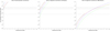 |
Fig. 1. Circularization timescale vs. orbital period in binary star systems. The black, red, blue, and green curves denote different laws of fast-tide suppression effects: in absence of suppression, and with linear, 5/3, and square laws, respectively. The horizontal dashed lines from bottom to top denote one-third of the age of the four open clusters from young to old: M 35 of 150 Myr, M 67 of 4 Gyr, NGC 188 of 7 Gyr, and Halo of 10 Gyr. |
4. Summary
We find that magnetic fields can significantly facilitate the tidal evolution of a binary system. This new physical mechanism arising from Ohmic dissipation rather than viscous dissipation leads to the order-of-magnitude change in the timescales of orbital evolution. Although in our estimations there are some uncertainties, for example magnetic fields, structure factors, convective velocity, and mixing length, our theory provides a good approach to understanding the tidal evolution of binary systems.
Acknowledgments
I thank Douglas N. C. Lin, Andrew Cumming, Xianfei Zhang and Tao Cai for their helpful discussions. This work is supported by National Natural Science Foundation of China (11872246, 12041301) and Beijing Natural Science Foundation (1202015).
References
- Bailey, A., & Goodman, J. 2019, MNRAS, 482, 1872 [NASA ADS] [CrossRef] [Google Scholar]
- Barker, A. J. 2020, MNRAS, 498, 2270 [Google Scholar]
- Bechter, E. B., Crepp, J. R., Ngo, H., et al. 2014, ApJ, 788, 2 [NASA ADS] [CrossRef] [Google Scholar]
- Brandenburg, A. 2016, ApJ, 832, 6 [Google Scholar]
- Cai, T. 2014, MNRAS, 443, 3703 [NASA ADS] [CrossRef] [Google Scholar]
- Chan, K. L., & Sofia, S. 1996, ApJ, 466, 372 [NASA ADS] [CrossRef] [Google Scholar]
- Christensen, U. R., Holzwarth, V., & Reiners, A. 2009, Nature, 457, 167 [Google Scholar]
- Davidson, P. A. 2013, Geophys. J. Int., 195, 67 [NASA ADS] [CrossRef] [Google Scholar]
- Duguid, C. D., Barker, A. J., & Jones, C. A. 2020, MNRAS, 497, 3400 [Google Scholar]
- Duquennoy, A., & Mayor, M. 1991, A&A, 500, 337 [NASA ADS] [Google Scholar]
- Fuller, J. W. 2014, PhD Thesis, Cornell University, USA [Google Scholar]
- Goldreich, P. 1963, MNRAS, 126, 257 [NASA ADS] [Google Scholar]
- Goldreich, P., & Nicholson, P. D. 1977, Icarus, 30, 301 [NASA ADS] [CrossRef] [Google Scholar]
- Goldreich, P., & Nicholson, P. D. 1989, ApJ, 342, 1079 [Google Scholar]
- Goldreich, P., & Soter, S. 1966, Icarus, 5, 375 [Google Scholar]
- Goodman, J., & Dickson, E. S. 1998, ApJ, 507, 938 [Google Scholar]
- Goodman, J., & Lackner, C. 2009, ApJ, 696, 2054 [Google Scholar]
- Goodman, J., & Oh, S. P. 1997, ApJ, 486, 403 [NASA ADS] [CrossRef] [Google Scholar]
- Hanasoge, S. M., Duvall, T. L., & Sreenivasan, K. R. 2012, Proc. Natl. Acad. Sci., 109, 11928 [Google Scholar]
- Hut, P. 1981, A&A, 99, 126 [NASA ADS] [Google Scholar]
- Jeffreys, H. 1961, MNRAS, 122, 339 [NASA ADS] [CrossRef] [Google Scholar]
- Jiang, J., Chatterjee, P., & Choudhuri, A. R. 2007, MNRAS, 381, 1527 [NASA ADS] [CrossRef] [Google Scholar]
- Käpylä, P. J., Rheinhardt, M., Brandenburg, A., & Käpylä, M. J. 2020, A&A, 636, A93 [NASA ADS] [CrossRef] [EDP Sciences] [Google Scholar]
- Kopal, Z. 1959, Close Binary Systems (New York: John Wiley& Sons) [Google Scholar]
- Lai, D. 1997, ApJ, 490, 847 [NASA ADS] [CrossRef] [Google Scholar]
- Lai, D., Helling, C., & van den Heuvel, E. P. J. 2010, ApJ, 721, 923 [NASA ADS] [CrossRef] [Google Scholar]
- Latham, D. W., Mathieu, R. D., Milone, A. A. E., & Davis, R. J. 1992, in Evolutionary Processes in Interacting Binary Stars, eds. Y. Kondo, R. Sistero, & R. S. Polidan, 151, 471 [NASA ADS] [Google Scholar]
- Li, S.-L., Miller, N., Lin, D. N. C., & Fortney, J. J. 2010, Nature, 463, 1054 [NASA ADS] [CrossRef] [Google Scholar]
- Lin, Y., & Ogilvie, G. I. 2018, MNRAS, 474, 1644 [Google Scholar]
- Lin, D. N. C., Bodenheimer, P., & Richardson, D. C. 1996, Nature, 380, 606 [Google Scholar]
- Maciejewski, G., Errmann, R., Raetz, S., et al. 2011, A&A, 528, A65 [NASA ADS] [CrossRef] [EDP Sciences] [Google Scholar]
- Maciejewski, G., Dimitrov, D., Fernández, M., et al. 2016, A&A, 588, L6 [NASA ADS] [CrossRef] [EDP Sciences] [Google Scholar]
- Mathieu, R. D. 1994, ARA&A, 32, 465 [NASA ADS] [CrossRef] [Google Scholar]
- Mayor, M., & Queloz, D. 1995, Nature, 378, 355 [Google Scholar]
- Meibom, S., & Mathieu, R. D. 2005, ApJ, 620, 970 [Google Scholar]
- Moffatt, H. K. 1978, Magnetic Field Generation in Electrically Conducting Fluids (Cambridge: Cambridge University Press) [Google Scholar]
- Ogilvie, G. I. 2014, ARA&A, 52, 171 [Google Scholar]
- Ogilvie, G. I., & Lin, D. N. C. 2004, ApJ, 610, 477 [Google Scholar]
- Patra, K. C., Winn, J. N., Holman, M. J., et al. 2017, AJ, 154, 4 [Google Scholar]
- Paxton, B., Bildsten, L., Dotter, A., et al. 2011, ApJ, 192, 3 [Google Scholar]
- Penev, K., Sasselov, D., Robinson, F., & Demarque, P. 2007, ApJ, 655, 1166 [Google Scholar]
- Penev, K., Sasselov, D., Robinson, F., & Demarque, P. 2009, ApJ, 704, 930 [NASA ADS] [CrossRef] [Google Scholar]
- Reiners, A., Schüssler, M., & Passegger, V. M. 2014, ApJ, 794, 144 [Google Scholar]
- Savonije, G. J., & Papaloizou, J. C. B. 1983, MNRAS, 203, 581 [Google Scholar]
- Terquem, C. 2021, MNRAS, 503, 5789 [NASA ADS] [CrossRef] [Google Scholar]
- Turner, J. D., Ridden-Harper, A., & Jayawardhana, R. 2021, AJ, 161, 72 [NASA ADS] [CrossRef] [Google Scholar]
- Vidal, J., & Barker, A. J. 2020, MNRAS, 497, 4472 [NASA ADS] [CrossRef] [Google Scholar]
- Wei, X. 2016, ApJ, 828, 30 [Google Scholar]
- Wei, X. 2018, ApJ, 854, 34 [Google Scholar]
- Wei, X. 2022, ApJ, 926, 40 [NASA ADS] [CrossRef] [Google Scholar]
- Weinberg, N. N., Arras, P., Quataert, E., & Burkart, J. 2012, ApJ, 751, 136 [NASA ADS] [CrossRef] [Google Scholar]
- Weinberg, N. N., Sun, M., Arras, P., & Essick, R. 2017, ApJ, 849, L11 [Google Scholar]
- Witte, M. G., & Savonije, G. J. 2002, A&A, 386, 222 [NASA ADS] [CrossRef] [EDP Sciences] [Google Scholar]
- Wright, N. J., Drake, J. J., Mamajek, E. E., & Henry, G. W. 2011, ApJ, 743, 48 [Google Scholar]
- Wu, Y. 2005, ApJ, 635, 674 [Google Scholar]
- Yousef, T. A., Brandenburg, A., & Rüdiger, G. 2003, A&A, 411, 321 [NASA ADS] [CrossRef] [EDP Sciences] [Google Scholar]
- Yu, L., Donati, J. F., Hébrard, E. M., et al. 2017, MNRAS, 467, 1342 [Google Scholar]
- Zahn, J. P. 1975, A&A, 41, 329 [NASA ADS] [Google Scholar]
- Zahn, J. P. 1977, A&A, 57, 383 [Google Scholar]
- Zahn, J. P. 1989, A&A, 220, 112 [Google Scholar]
- Zanazzi, J. J. 2022, ApJ, 929, L27 [NASA ADS] [CrossRef] [Google Scholar]
- Zanazzi, J. J., & Wu, Y. 2021, AJ, 161, 263 [NASA ADS] [CrossRef] [Google Scholar]
Appendix A: Estimation of electric current
In this section we first illustrate why the turbulent Ohmic dissipation is ∼J2/σt. According to the mean field theory for magnetohydrodynamic (MHD) turbulence (Moffatt 1978), the correlation of turbulent convective velocity v′ and turbulent magnetic field B′ (i.e., turbulent electromotive force) can be modeled with the large-scale field B
 (A.1)
(A.1)
where the coefficients α and β are pseudo-tensors for anisotropic turbulence, but scalars for isotropic turbulence in our simple analysis. The coefficient α is related to fluid helicity v′ × (∇ × v′) and the terminology “α effect” in dynamo theory arises from this coefficient. Inserting the mean field theory into the magnetic induction equation we can derive magnetic diffusion to be (η + β)∇2B, where η = 1/(σμ) is the laminar magnetic diffusivity. We denote β = ηt and in turbulence ηt ≫ η (i.e., magnetic diffusion ≈ηt∇2B). We then introduce turbulent electric conductivity σt so that ηt = 1/(σtμ). We now perform the dot product with B/(2μ) on the magnetic induction equation
to derive magnetic energy equation. The Ohmic dissipation arises from the last term,
 (A.2)
(A.2)
where the vector identities ∇2B = −∇ × (∇ × B) and ∇ ⋅ (B × J)=J ⋅ (∇ × B)−B ⋅ (∇ × J) are employed. In (A.2) the first term ∇ ⋅ (B × J) almost vanishes for a volume integral over convection zone, and the second term is the turbulent Ohmic dissipation ∼J2/σt.
Next we derive why the electric current J associated with tide is ∼σtuB. The electric current J associated with tidal flow u is calculated by Ohm’s law
 (A.3)
(A.3)
where E is the electric field associated with tidal flow, B is the mean field generated by dynamo in stellar convection zone, and b is the field induced by tidal flow u. It should be noted that the mean field B is associated with a strong electric current in dynamo action, but what we are concerned with is not this current due to turbulent convection, but the current J associated with tidal flow u. In this sense, B is assumed to be steady and potential for the sake of simplicity (it is possible to involve the dynamo-generated current in the following analysis, but it is irrelevant to our calculation of tidal dissipation). To make the order-of-magnitude estimations, we introduce the length scale lb associated with the tidally induced field b, which should be much less than the large-scale R, which is the stellar radius. Ampere’s law μJ = ∇ × b gives the estimation J ≃ b/(μlb). Faraday’s law states ∇ × E = −∂b/∂t. The electric field is caused by the tidal flow on the length scale lb and the timescale of b is tidal period τ. Thus, Faraday’s law yields the estimation E ≃ blb/τ. We now estimate each term in Ohm’s law (A.3)
 (A.4)
(A.4)
where the first row shows the four terms labeled with circled numbers and the second row shows the estimations. Then we build the balance among these terms. It is impossible that the four terms are at the same order, because ③ and ④ cannot be comparable since b ≪ B (i.e., the tide cannot be as strong as the convection). It is also impossible that the three terms are at the same order because the left term cannot be balanced. Thus, the only possibility is that two terms are in balance and the other two are in balance. Then there are three combinations: ① ≃ ② and ③ ≃ ④; ① ≃ ③ and ② ≃ ④; ① ≃ ④ and ② ≃ ③. The first combination cannot hold since b ≪ B (i.e., ③ ≃ ④ cannot hold). In the second combination, ② ≃ ④ leads to lb ≃ uτ ≃ ξ, and ① ≃ ③ leads to b/B ≃ ulb/ηt ≃ uξ/ηt. In the third combination, ① ≃ ④ leads to ηt ≃ ulb, and ② ≃ ③ leads to b/B ≃ uτ/lb ≃ ξ/lb ≃ uξ/ηt. We now compare these two combinations. Both combinations yield b/B ≃ uξ/ηt, which is reasonable because a stronger tide corresponds to a higher ratio b/B. However, the difference between the two combinations is that lb ≃ ξ in the second combination, whereas lb ≫ ξ (i.e., b/B ≃ ξ/lb) in the third combination. By definition, lb is the length scale associated with the tidally induced field b. Therefore, it is reasonable that lb should be comparable to tide ξ, but cannot be much larger than the tide. Finally, we chose the second combination in which J ≃ b/(μlb)≃σtuB.
All Tables
Calculation results for the 51 Pegasi b system. The stellar surface field is 1000 gauss.
All Figures
|
Fig. 1. Circularization timescale vs. orbital period in binary star systems. The black, red, blue, and green curves denote different laws of fast-tide suppression effects: in absence of suppression, and with linear, 5/3, and square laws, respectively. The horizontal dashed lines from bottom to top denote one-third of the age of the four open clusters from young to old: M 35 of 150 Myr, M 67 of 4 Gyr, NGC 188 of 7 Gyr, and Halo of 10 Gyr. |
| In the text | |
Current usage metrics show cumulative count of Article Views (full-text article views including HTML views, PDF and ePub downloads, according to the available data) and Abstracts Views on Vision4Press platform.
Data correspond to usage on the plateform after 2015. The current usage metrics is available 48-96 hours after online publication and is updated daily on week days.
Initial download of the metrics may take a while.