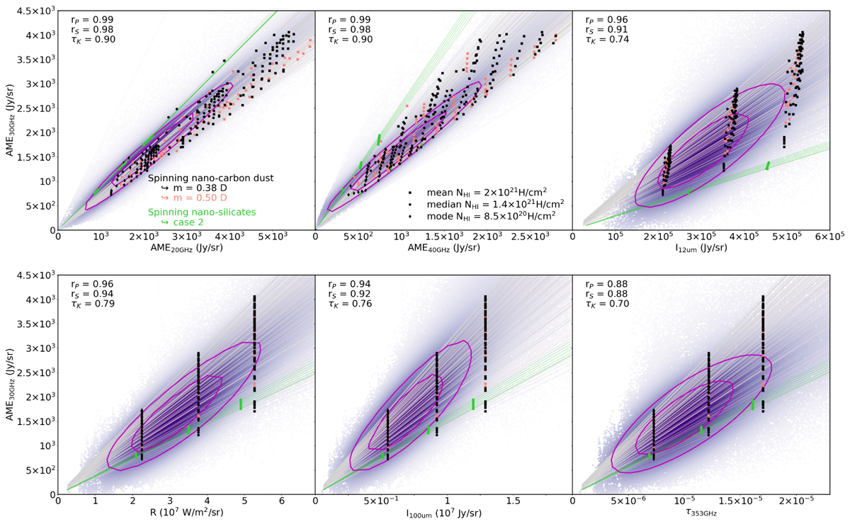
Comparison of observed and modelled correlations. Top from left to right: observations are plotted as density of points maps of AME_{30 GHz} vs. AME_{20 GHz}, vs. AME_{40 GHz}, and vs. dust emission in the 12 μm IRAS filter. Bottom from left to right: observations are plotted as density of points maps of AME_{30 GHz} vs. radiance, vs. dust emission in the 100 μm IRAS filter, and vs. optical depth at 353 GHz. For all panels, we overplot the contours enclosing 50% of the pixels (internal contour) and 75% of the pixels (external contour). The models fitting the observations are shown with black and pink symbols for spinning nano-carbon dust, m = 0.38 and 0.5 D, respectively, and green symbols for spinning nano-silicate dust (case 2; see Sect. 5 for details). Squares, circles, and diamonds show models scaled to the mean (N_HI = 2 × 10²¹ H cm^–2), the median (N_HI = 1.4 × 10²¹ H cm^–2), and the mode HI column density (N_HI = 8.5 × 10²⁰ H cm^–2), respectively. The light grey, pink, and green lines show the same models for HI column densities extending over the entire observational range 10²⁰ ⩽ N_HI ⩽ 1.4 × 10²² H cm^–2. The various model points show spinning-dust models for different f_CNM values (see Sect. 5.2 for details). The r_P, r_S, and τ_K give the Pearson correlation coefficient, the Spearman rank-order correlation coefficient, and the Kendall’s tau, respectively.