© ESO 2022

1. Introduction

Binary pulsars are the natural laboratory of general relativity (GR) in the strong-field regime. High-precision pulsar timing can measure not only the Keplerian orbital parameters, but also the relativistic correction to the Keplerian orbit, which is parameterized to the five post-Keplerian (PK) parameters, that is to say the orbital decay Ṗ_b, the periastron advance $\dot{\omega }$, the Einstein delay γ, the range r, and the shape s of the Shapiro delay (Zhang et al. 2019, and references therein). The most studied parameter, Ṗ_b, has been treated containing only two effects besides GR (Zhu et al. 2018). One is the Shklovskii kinematic effect originating in the transverse motion of a pulsar binary (Shklovskii 1970), and the other is the Doppler effect induced by the acceleration along the line of sight of the pulsar binary. After subtracting these effects, the remnant should be the gravitational wave (GW) radiation term originating in GR. However, the remnant Ṗ_b of some pulsar binaries becomes positive which is inconsistent with the prediction of the GW (Pathak & Bagchi 2019), which suggests the involvement of other mechanisms such as wind accretion, tidal dissipation, and magnetic braking. Therefore, the situation becomes complicated. It is thereby worth further investigation to determine the true GW term.

Here, the timing results of all pulsar binaries with the measured derivative of the orbital period are collected, except for binary pulsars with an orbital eccentricity larger than 0.1 and for neutron star-neutron star binaries. Interestingly, all systems are millisecond pulsar binaries. By carefully subtracting the kinematic term, the acceleration term, and the GW term, the residual term of these pulsar binaries is found to be roughly half positive and half negative. Further, the possibility of such a distribution originating from tidal dissipation is investigated.

Tidal dissipation is usually ignored or not discussed in depth in most millisecond pulsar (MSP-) white dwarf (WD) binaries. It has been thought that the companion has already been synchronized with the orbit or that tidal dissipation is too weak on a WD to have any noticeable effects (Freire et al. 2012; Antoniadis et al. 2013). However, all MSP systems have experienced the recycled stage (Lorimer 2008), so it is still uncertain whether the spin of the companion star has already been synchronized with the orbit after the recycled stage. On the other hand, although the equilibrium tide has been thought to be responsible for the tidal effect on a WD (Applegate & Shaham 1994), which is usually weak, dynamical tidal dissipation on a WD can be more efficient than equilibrium tidal dissipation (Fuller & Lai 2012). Hence, it is worth revisiting the possibility of tidal dissipation induced Ṗ on these systems.

To evaluate the effect of tidal dissipation on pulsar binaries, the tidal parameters of every system are calculated. Furthermore, we show that the dynamical tide on a WD is efficient enough to produce the maximum tidal parameter in MSP-WD systems. Additionally, the tidal parameter of MSP-MS system PSR J1227-4853 corresponds to a reasonable Love number $k_2=0.{177}_{-0.058}^{+0.098}$ of a MS companion under the equilibrium tide model. These results likely support the idea that tidal dissipation is also a non-negligible contributor to the Ṗ_b of MSP binaries, with the equilibrium tidal model responsible for the MS companion and the dynamical tidal model responsible for the WD companion.

Moreover, a weak power-law correlation between the tidal parameter and the orbital period is found in MSP-WD binaries. Compared with the general tidal model, such a correlation requires that the spin of the companion correlates with the orbital frequency in millisecond pulsar binaries, which possibly results from binary evolution.

This paper is organized as follows: The estimation of the residual ${\dot{P}}_b^{\mathrm{Res}}$ in all systems is described in Sect. 2. The comparison of the tidal parameters of these systems with tidal models is presented in Sect. 3. The discussion and conclusion are drawn in Sects. 4 and 5.

2. Samples collection and Ṗ_b calculations

2.1. The general components of observational Ṗ_b

The observed Ṗ_b from pulsar timing is the sum of different effects. It is contaminated by two kinematic effects, with one being the Shklovskii kinematic effect originating in the transverse motion of a pulsar binary (Shklovskii 1970):

$$\begin{array}{c}\hfill {\dot{P}}_b^{\mathrm{Shk}}={\mu }_{\perp }^2\frac{D}{c}{P}_b.\end{array}$$(1)

Here μ_⊥ is the total proper motion velocity, P_b is the orbital period, D is the distance of the binary, and c is the speed of light. The other effect contributing to the measured P_b stems from the acceleration of the pulsar along the line of sight:

$$\begin{array}{c}\hfill {\dot{P}}_b^{\mathrm{Acc}}=\frac{A}{c}{P}_b,\end{array}$$(2)

where A is the acceleration along the line of sight. In subtracting these two terms as shown in Eqs. (1) and (2) from the observed one, we obtain the intrinsic ${\dot{P}}_b^{\mathrm{Int}}$, which is considered to be dominated by gravitational radiation so that ${\dot{P}}_b^{\mathrm{Int}}={\dot{P}}_b^{\mathrm{GW}}$, where

$$\begin{array}{c}\hfill {\dot{P}}_b^{\mathrm{GW}}=-\frac{192\pi P_b^{-5/3}{G}^{5/3}{m}^{4/3}{m}_{\mathrm{p}}{m}_{\mathrm{c}}}{5{(2\pi )}^{-5/3}{c}^5}(1+\frac{73}{24}{e}^2+\frac{37}{96}{e}^4){(1-e^2)}^{-7/2}.\end{array}$$(3)

Here G is the gravitational constant; m is the total mass of binary; m_p and m_c are the mass of the pulsar and companion star, respectively; and e is the orbital eccentricity.

2.2. Pulsar binary data

To test the effect on Ṗ_b other than ${\dot{P}}_b^{\mathrm{Shk}}$, ${\dot{P}}_b^{\mathrm{Acc}}$, and ${\dot{P}}_b^{\mathrm{GW}}$ mentioned above, all pulsar binaries with Ṗ_b detected within a 3σ significance and of a relatively low eccentricity (e < 0.1) were collected, excluding the double neutron star system. There are 26 pulsar binaries available and all of them are millisecond pulsar binaries. The measured parameters of those sources are shown in Table A.3. A detailed discussion of these parameters is given in the following.

Among the 26 sources, two sources are the main-sequence star (MS) millisecond pulsar binaries; 17 are PSR-WD systems; and the remaining seven sources have no optical counterpart or the type of their companion star cannot be determined by the optical observation, which suggests that the companions of these pulsars are faint. Those uncertain companions are thus assumed to be WDs.

2.3. The estimation of the kinematic term in Ṗ_b

The estimation of ${\dot{P}}_b^{\mathrm{Shk}}$ and ${\dot{P}}_b^{\mathrm{Acc}}$ from Eqs. (1) and (2) requires the distance, proper motion, and acceleration of the systems. In our samples, almost all binaries have a measured proper motion, except PSR J1701-3006B and PSR J1807-2459A. The proper motion of PSR J2222-0137 is measured by the very long baseline interferometry (VLBI; Deller et al. 2013), the proper motion of PSR J1227-4853 and PSR J1957+2516 are measured by Gaia (Gaia Collaboration 2018), and the proper motion of the remaining sources are given by pulsar timing.

On the distance measurement of the 26 sources, two pulsars have a precise distance measurement, one being PSR J2222-0137 which was measured by VLBI (Deller et al. 2013) and the other one being PSR J1227-4853 which was measured by Gaia (Gaia Collaboration 2018). For the remaining 24 sources, the distance of ten pulsar binaries is given by the pulsar timing via a parallax, and the remaining sources have no distance measurement. As 11 pulsars are located in the globular clusters, their distance can be estimated by the distance of the globular clusters given by Baumgardt (Baumgardt et al. 2018). For the remaining three pulsars with the absence of all those methods for the distance measurement mentioned above, their distance was estimated by their dispersion measure (DM) and YMW16 galactic electron density model (Yao et al. 2017), which can be found by the “DIST_DM” parameter from the Australia Telescope National Facility (ATNF) pulsar catalog (Manchester et al. 2005). For these systems, a 1σ uncertainty is assumed to be 20% of the corresponding distance value.

The acceleration of a pulsar is normally attributed to the galactic potential, which can be calculated by McMillan’s model (McMillan 2017). For binaries in the globular clusters, the potential of the cluster also contributes to the acceleration of the pulsar binary, which can be calculated by the simple globular cluster model of Freire (Freire et al. 2005).

In Freire’s model, the potential of the globular cluster can be expressed by the density and radius of the core of the cluster, which has been estimated by Baumgardt for all globular clusters (Baumgardt et al. 2018). Then the acceleration along the line of sight only depends on z, the distance between the point and the sky plane through the center of the cluster, which cannot be measured. By searching the largest possible range, the acceleration has a maximum $A_{max}^{\mathrm{gc}}$ and a minimum $A_{min}^{\mathrm{gc}}$, which has the same magnitude but an opposite direction. We assume that the probability distribution of the line-of-sight acceleration in globular clusters is described by the Gaussian distribution with a mean value 0 and a standard deviation of $A_{max}^{\mathrm{gc}}/3$.

Now, the contribution of the Shklovskii and acceleration effect to ${\dot{P}}_b^{\mathrm{int}}$ can be calculated by Eqs. (1) and (2), respectively. After subtracting two kinematic effects from the measured one, ${\dot{P}}_b^{\mathrm{Obs}}$, the intrinsic orbital decay, ${\dot{P}}_b^{\mathrm{Int}}$, can be obtained,

$$\begin{array}{c}\hfill {\dot{P}}_b^{\mathrm{Int}}={\dot{P}}_b^{\mathrm{Obs}}-{\dot{P}}_b^{\mathrm{Shk}}-{\dot{P}}_b^{\mathrm{Acc}}.\end{array}$$(4)

Such an intrinsic ${\dot{P}}_b^{\mathrm{int}}$ should be dominated by the gravitational radiation term. However, a considerable number of systems show positive ${\dot{P}}_b^{\mathrm{int}}$, which is inconsistent with the prediction of GW radiation, expecting a negative Ṗ_b only. Most probably, ${\dot{P}}_b^{\mathrm{int}}$ is contaminated by an effect other than the two terms at the right-hand side of the above equation.

2.4. The residual ${\dot{\mathsf{P}}}_{\mathsf{b}}^{\mathsf{Res}}$

To figure out such an effect, we need to subtract the gravitational radiation-induced orbital changing ${\dot{P}}_b^{\mathrm{GW}}$ from the intrinsic one, which is ${\dot{P}}_b^{\mathrm{Res}}={\dot{P}}_b^{\mathrm{Int}}-{\dot{P}}_b^{\mathrm{GW}}$. Such a residual ${\dot{P}}_b^{\mathrm{Res}}$ reflects the behavior of the unknown effect, which can be examined in terms of significance.

To calculate the term of gravitational radiation given by Eq. (3), the orbital eccentricity and masses of double stars are necessary. The eccentricity can be measured by pulsar timing. For binaries without an eccentricity measurement, the nondetection means that the eccentricity is very small and can be treated as zero.

The companion mass, m_c, pulsar mass, m_p, and orbital inclination, i, are related to the mass function f(m_c) by

$$\begin{array}{c}\hfill f(m_{\mathrm{c}})=\frac{m_{\mathrm{c}}^3{sin}^{3}i}{{(m_{\mathrm{p}}+m_{\mathrm{c}})}^2}.\end{array}$$(5)

Such a mass function can be measured by pulsar timing for all sources. The orbital inclination and companion mass can be given by the measurement of the Shapiro delay. However, the Shapiro delay has only been detected in five binaries in our samples. And there are four binaries with mass ratios measured by their radial velocities (see Table A.1).

To estimate the mass of double stars, three assumptions are made. For all binaries without a Shapiro delay detection, the pulsar mass is assumed to be 1.48 ± 0.2 M_⊙, given the statistics result (Özel et al. 2012). For the binaries with neither a Shapiro delay detection nor a mass ratio measurement, the direction of the orbit is assumed to be isotropic, corresponding to a probability density function of orbital inclination P(i) = sin i. And the minimum mass of the companion of all binaries is assumed to be 0.08 M_⊙.

Thus, the gravitational radiation-induced ${\dot{P}}_b^{\mathrm{GW}}$ can be obtained by Eq. (3). After subtracting it from the intrinsic one, ${\dot{P}}_b^{\mathrm{Int}}$, we determined the residual term, ${\dot{P}}_b^{\mathrm{Res}}$. All components of Ṗ_b from our sample are shown in Table A.3.

We did not use the standard technique of statistical error propagation because the non-Gaussian probability density function was adopted in the estimation for the mass and the acceleration was calculated by the code from McMillan’s model (McMillan 2017), which does not include error propagation. Thus, the uncertainty of ${\dot{P}}_b^{\mathrm{Res}}$ was calculated by the Monte Carlo method. The middle value was estimated by the 50th percentile of the sampling result, and the 1σ lower and upper uncertainty was estimated by the 17.37th and 82.63th percentile of the sampling result, respectively. The same method was applied to the uncertainty estimation of the following calculations.

The significance of the residual ${\dot{P}}_b^{\mathrm{Res}}$ is within 1σ for 21 binaries, 2σ for 14 binaries, and 3σ for nine binaries as shown in Fig. 1. The uncertainty of ${\dot{P}}_b^{\mathrm{Res}}$ mainly stems from the measurement for the distance. As shown in Table A.3, for the majority of systems, ${\dot{P}}_b^{\mathrm{Obs}}$ is close to their ${\dot{P}}_b^{\mathrm{Shk}}$. The uncertainty of the distance measurement by pulsar timing is usually large, corresponding to a large uncertainty on ${\dot{P}}_b^{\mathrm{Res}}$.

Fig. 1. Relationship between $|{\dot{P}}_b^{\mathrm{Res}}|$ and orbital period Pb in logarithmic coordinates. Only the systems with ${\dot{P}}_b^{\mathrm{Res}}$ in 1σ significance are shown. Different colors represent the binaries of the different ways of the distance measurements1. The solid symbols denote systems with positive ${\dot{P}}_b^{\mathrm{Res}}$ and the hollow ones represent sources with negative ${\dot{P}}_b^{\mathrm{Res}}$. The line is the fitting by the power law relation of systems with a WD companion.

Such a residual ${\dot{P}}_b^{\mathrm{Res}}$ reflects the behavior of the unknown effect. Among 21 binaries, eleven sources have positive values for ${\dot{P}}_b^{\mathrm{Res}}$ and ten sources have negative ones. The half-to-half distribution of ${\dot{P}}_b^{\mathrm{Res}}$ is easy to understand in the scenario for random noise, whereas the possibility of the tidal effect on the residual ${\dot{P}}_b^{\mathrm{Res}}$ discussed in the following section provides another scenario that may lead to such a distribution.

3. The comparison with the tidal model

3.1. Tidal models

Considering a circular binary containing a companion star with radius R_c and mass m_c and a primary star with mass m_p treated as a point mass, the companion star is deformed by the tidal potential of the primary star, then the deformation of the companion star produces an extra torque and disturbs the motion of the binary. The first derivative of the orbital period due to tidal torque can be expressed as

$$\begin{array}{c}\hfill {\dot{P}}_b=\frac{3T{P}_b^2}{2\pi \mu a^2}.\end{array}$$(6)

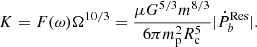
Here μ = m_pm_c/(m_p + m_c) is the reduced mass, a is the orbital semi-major axis, and T is the tidal torque, which can be parameterized as (Fuller & Lai 2012)

$$\begin{array}{c}\hfill T=T_{0}F(\omega )\mathrm{sgn}(\omega ).\end{array}$$(7)

Here T₀ is $G{(m_{\text{p}}/a^3)}^2{R}_{\text{c}}^5$, representing the effect of the external field, and F(ω) is the response of the companion star to the gravity exerted by the primary star, which is usually denoted as a dimensionless function of tidal frequency ω = Ω_c − Ω (defined as the difference between the orbital frequency Ω and spin frequency Ω_c), and the direction of torque only depends on the sign of the tidal frequency.

For the general binaries, the formula for F(ω) also depends on the tidal frequency, the eccentricity, the inclination between the spin of the companion star and orbit, and the interior physics of the companion star (Ogilvie 2014). If the orbit is circular and if the inclination is small, the eccentric and oblique terms in the tidal response vanish, thus F(ω) only depends on the tidal frequency and interior physics of the star.

There are two kinds of tidal models (Ogilvie 2014). One kind is the equilibrium tide in which a star is in hydrostatic equilibrium, and the other is the dynamical tide in which a star is treated as an oscillator in various modes.

The tidal dissipation of equilibrium tide is normally attributed to the turbulent viscosity in the convection zone, which is the most powerful mechanism of energy dissipation (Zahn 1989). In such a model, the dimensionless tidal response is inversely proportional to the convection friction time t_f = (MR²/L)^1/3 and proportional to the tidal frequency

$$\begin{array}{c}\hfill F(\omega )=3\frac{k_2}{t_f}\frac{\omega }{{\mathrm{\Omega }}_k^2}\sqrt{\frac{320}{320+{\eta }^2}}.\end{array}$$(8)

Here ${\mathrm{\Omega }}_k={(G{m}_{\mathrm{c}}/R^3)}^{\frac{1}{2}}$ is THE dynamical frequency of the companion star, coefficient k₂ is THE Love number of the companion star, and η = t_fω/π (Zahn 1989; Goupil & Zahn 2008).

Even though the Zahn’s equilibrium tide model is for the MS, it had been widely applied to the investigation of WD tidal dissipation (Freire et al. 2012; Antoniadis et al. 2013). The more sophisticated model, that is to say the dynamical model for the WD had been discussed by Fuller (Fuller & Lai 2012, 2013), and it can produce more efficient tidal dissipation, especially at a high tidal frequency.

In this model, the excitation and dissipation of excited gravity waves in the star are involved, and the outgoing propagating waves can be efficiently damped in the outer layer of the star by the nonlinear mechanism. Fuller numerically simulated the dynamical tide on the WD and found the tidal response F(ω) satisfied

$$\begin{array}{c}\hfill F(\omega )\propto {\omega }^5\end{array}$$(9)

for a carbon-oxygen WD, and

$$\begin{array}{c}\hfill F(\omega )\propto {\omega }^6\end{array}$$(10)

for a helium WD.

If the residual Ṗ_b originated in the tide dissipation, the magnitude of the tidal response F(ω) should be consistent with the tidal model. In such a case, ${\dot{P}}_b^{\mathrm{Res}}$ can also set a constraint on the interior of the companion on pulsar binaries.

3.2. On the value of F(ω)

By combining Eqs. (6) and (7), the tidal response F(ω) can be calculated as

$$\begin{array}{c}\hfill F(\omega )=\frac{\mu a^{\mathbf{8}}{\mathrm{\Omega }}^2}{6\pi G{m}_{\mathrm{p}}^2{R}_{\mathrm{c}}^5}|\dot{P_b^{\mathrm{Res}}}|=\frac{\mu G^{5/3}{m}^{8/3}{\mathrm{\Omega }}^{-10/3}}{6\pi m_{\mathrm{p}}^2{R}_{\mathrm{c}}^5}|\dot{P_b^{\mathrm{Res}}}|,\end{array}$$(11)

where Ω = (2π/P_b) is the orbital frequency.

The calculation of F(ω) of all systems from Eq. (6) requires knowledge on the radius of the companion, which can be obtained by the analytic relation between the mass and radius of WDs (Andronov & Yavorskij 1990):

$$\begin{array}{c}\hfill \frac{R_{\mathrm{c}}}{R_{\odot }}=0.01153{({\left(\frac{m_{\mathrm{c}}}{1.44M_{\odot }}\right)}^{-\frac{2}{3}}-{\left(\frac{m_{\mathrm{c}}}{1.44M_{\odot }}\right)}^{\frac{2}{3}})}^{0.465}.\end{array}$$(12)

For the MS companion, we used the empirical formula of the mass-radius relation (Demircan & Kahraman 1991):

$$\begin{array}{c}\hfill \frac{R_{\mathrm{c}}}{R_{\odot }}=1.06{\left(\frac{m_{\mathrm{c}}}{M_{\odot }}\right)}^{0.945}.\end{array}$$(13)

In order to check whether the F(ω) of systems are expected by the tidal model or not, tidal frequencies are required. However, they are unknown for all PSR-WD binaries because the rotation velocity of those companions is not measurable. Therefore, the tidal model can only impose an upper limitation on F(ω) for those systems.

The maximum F(ω) among all the systems is about 10³, corresponding to a convection friction time t_f ≈ 6 × 10⁻¹² year in Zahn’s equilibrium model. Such a friction time corresponds to an impossibly large luminosity of $L=G{M}^2/t_f^3\approx {10}^{28}{L}_{\odot }$ L_⊙. Therefore, Zahn’s equilibrium tide dissipation is too weak to explain the F(ω) of the pulsar binaries.

In contrast, in Fuller’s dynamical tide model, the maximum magnitude of F(ω) is about 40 for helium WD and 10⁵ for carbon-oxygen WD in the case that companion rotates with break-up velocity. Such an upper limit for F(ω) is larger than the maximum one of all the systems. Therefore, the dynamical tide can provide a sufficient tidal response for these systems.

If the spin of the companion can be measured, the F(ω) can be obtained and compared with the tidal model. PSR J1227-4853 is a millisecond pulsar binary with a MS companion, the projected rotation velocity of which was measured through spectrum broadening v_c = 86 ± 20 km s⁻¹ (de Martino et al. 2014). The spin of the companion can thus be obtained by ${\mathrm{\Omega }}_{\mathrm{c}}=v_{\mathrm{c}}/R_{\mathrm{c}}sini={41}_{-9}^{+10}{\mathrm{rad}\mathrm{day}}^{-1}$, and the inclination i and radius R_c was obtained by the same method as in Sect. 2.3.

The convection friction time of the companion of PSR J1227-4853 in Zahn’s tidal model is

$$\begin{array}{c}\hfill t_f={(M{R}^2/L)}^{1/3}=0.26\pm 0.01\text{year},\end{array}$$(14)

where the luminosity was obtained by the temperature 6100 K (de Martino et al. 2014), assuming the radiation is a blackbody. If ${\dot{P}}_b^{\mathrm{Res}}$ is caused by the tidal dissipation of Zahn’s equilibrium tide model, it implies a tidal response of $F(\omega )=1.3_{-0.41}^{+0.67}\times {10}^{-7}$, which yields a Love number for the companion star of 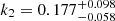$k_2=0.{177}_{-0.058}^{+0.098}$. Such a Love number is a reasonable value for the MS. Consequently, the ${\dot{P}}_b^{\mathrm{Res}}$ of the MS-MSP binaries can be explained by Zahn’s model of equilibrium tide.

The tidal model can not be tested directly due to the lack of companion rotation velocity in the PSR-WD systems. As the maximum F(ω) among these PSR-WD binaries can be achieved by the dynamical tidal model with a reasonable rotation velocity, the contribution of the tidal dissipation to the orbital decay Ṗ_b of the systems cannot be excluded yet. On the other hand, a reasonable Love number for the MS companion of PSR J1227-4853 inferred by Eq. (8) can be regarded as supporting evidence for the equilibrium tide on the PSR-MS systems.

3.3. A possible correlation

We also find a possible correlation between the tidal response parameter F(ω) and the orbital period P_b. To analyze the tidal dissipation of these systems, a new tidal parameter K rather than F(ω) was adopted:

$$\begin{array}{c}\hfill K=F(\omega ){\mathrm{\Omega }}^{10/3}=\frac{\mu G^{5/3}{m}^{8/3}}{6\pi m_{\mathrm{p}}^2{R}_{\mathrm{c}}^5}|{\dot{P}}_b^{\mathrm{Res}}|.\end{array}$$(15)

As F(ω) is dependent on P_b, the correlation analysis of tidal parameters and the orbital period is affected. In contrast, the calculation of K only uses ${\dot{P}}_b^{\mathrm{Res}}$ and the mass of a binary system, which is more suitable for the tidal analysis.

Upon obtaining the tidal parameter K, a weak positive correlation emerged as shown in Fig. 2. Thus the Pearson correlation coefficient between log P_b and log K of MSP-WD systems can be obtained and it exhibits a quantitative evaluation of such a correlation. As different methods of the distance measurement affect the reliability of the result, the Pearson correlation coefficient of $log|{\dot{P}}_b^{\mathrm{Res}}|$ and log P_b is shown in Table 1, which is apparently influenced by the different ways used to measure the distance.

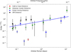Fig. 2. Relationship between K and orbital period Pb in logarithmic coordinates. Only systems with ${\dot{P}}_b^{\mathrm{Res}}$ above a 1σ significance are shown. The meaning of the point style is the same as in Fig. 1.

As shown in Table 1, the Pearson correlation coefficients of log K and log P_b imply that there is a weak correlation between them in different combinations of the distance measurement and significance levels. Such a correlation likely does not originate in the correlation between $log|{\dot{P}}_b^{\mathrm{Res}}|$ and log P_b due to their small Pearson correlation coefficients. As the correlation is strongly affected by the point at the top right of the Fig. 2, we carried out the same analysis without that point as shown in Table 2. In such a case, the only difference from the previous analysis is that the correlation between ${\dot{P}}_b^{\mathrm{Res}}$ and P_b in the 3σ significance exhibits a significant enhancement. Nevertheless, the Pearson correlation coefficients of log K and log P_b still show a weak correlation between them, as shown in the previous case.

A strong correlation between ${\dot{P}}_b^{\mathrm{Res}}$ and P_b is also shown in the pulsar binaries of the s. Such a systematic correlation probably stems from the assumption that the acceleration of the globular clusters satisfies the Gaussian distribution with a mean value 0 and a standard deviation $a_{max}^{\mathrm{gc}}/3$. As the correlation coefficient was calculated by the middle value of the data, ${\dot{P}}_b^{\mathrm{Acc}}$, which is proportional to the orbital period, may not have been correctly estimated in calculations of the Pearson correlation coefficient. Nevertheless, the strong correlation favors the existence of universal tidal dissipation in the majority of MSP-WD systems.

Fitting with a simple power-law relation $K=\alpha P_b^{\beta }$ was carried out for MSP-WD systems, as shown in Table 3. The probability density distribution of K and ${\dot{P}}_b^{\mathrm{Res}}$ is non-Gaussian, which was thus analyzed by the Monte Carlo method. The steps are as follows: the values of K or ${\dot{P}}_b^{\mathrm{Res}}$ were sampled on the basis of their probability density distribution, and a classical linear regression in logarithmic coordinates for those values was performed. After repeating such a process 100 000 times, the distribution of the slope and intercept was obtained, which exhibits a Gaussian distribution. The reduced Chi-square was calculated by taking the mean of the upper and lower uncertainty at a 1σ level.

Such a correlation between K and P_b indicates that ${\dot{P}}_b^{\mathrm{Res}}$ originates in tidal dissipation in the majority of MSP-WD systems. For the MSP-MS systems, only two systems are available, and the origin of ${\dot{P}}_b^{\mathrm{Res}}$ for them cannot be judged by this correlation. The possible origin of this correlation is further discussed in Sect. 4.2.

4. Discussion

4.1. The effect of the winds

The change in system mass can also affect the orbital period. For the circular binary, the derivative of the orbital period due to the change of mass is (Tout & Hall 1991)

$$\begin{array}{cc}& {\dot{P}}_b^{\dot{m}}=-2\frac{\dot{m}}{m}{P}_b+\frac{3{\dot{m}}_{\mathrm{p}}(m_{\mathrm{p}}-m_{\mathrm{c}})}{m_{\mathrm{p}}{m}_{\mathrm{c}}}{P}_b\hfill \\ \hfill & =-2\frac{{\dot{m}}_{\mathrm{c}}}{m}{P}_b+\frac{{\dot{m}}_{\mathrm{p}}(3m{m}_{\mathrm{p}}-3m{m}_{\mathrm{c}}-2m_{\mathrm{p}}{m}_{\mathrm{c}})}{m{m}_{\mathrm{p}}{m}_{\mathrm{c}}}{P}_b,\hfill \end{array}$$(16)

where ṁ = ṁ_c + ṁ_p is total mass loss.

All systems of our samples are detached binaries, so the transfer and loss of mass can only possibly come from the winds’ accretion. In the simple case that the pulsar does not accrete winds (ṁ_p = 0), the derivative of the orbital period is

$$\begin{array}{c}\hfill {\dot{P}}_b^{\dot{m}}=-2\frac{{\dot{m}}_{\mathrm{c}}}{m}{P}_b.\end{array}$$(17)

Such a ${\dot{P}}_b^{\dot{m}}$ is always positive because ṁ_c < 0.

The material in the atmosphere of the star can escape from the surface driven by the radiation and produce winds. The existence of stellar wind is often seen in MS. For the WD, the winds only exist in the hot WD (Unglaub 2008). In all WD-MSP binaries with a measured companion temperature, PSR J0024-7204U has the highest companion temperature of about 12 000 K (Cadelano et al. 2015). So all WDs that have a measured temperature in our samples are not hot and cannot produce winds. For these WDs for which temperature has not been measured, the mass of winds cannot be estimated.

On the other hand, the winds can also be driven by the radiation from the pulsar (Freire et al. 2012). The mass of such winds depends on the power of the radiation from the pulsar, which can be estimated by the intrinsic spin-down. By assuming the total energy release of the pulsar that is received by the companion, the upper limit of the mass of the winds can be estimated. The intrinsic spin-down was calculated from the observational one after subtracting the kinematic effects. This complicates the analysis.

We adopted a simpler method to estimate the mass of the winds via the modulation of the DM (Freire et al. 2012). The winds can produce an extra column density along the line of sight, and thus disturb the observational DM. This method does not depend on the companion type or the origin of the radiation driving the winds.

By assuming the isotropic winds of the WD, the mass loss was obtained by

$$\begin{array}{c}\hfill {\dot{m}}_{\mathrm{c}}=-2\pi X{\mu }_{\mathrm{p}}{v}_{0}a\frac{sini}{i}\mathrm{\Delta }H.\end{array}$$(18)

Here v₀ is the velocity of the wind, X is the number of nucleons per electron, μ_P is the proton mass, and ΔH is the amplitude of the column density modulation which can be related to the DM modulation by ΔH = ΔDM × 3.0857 × 10¹⁸ cm pc⁻¹.

For a rough estimation, we assumed that the 1σ measurement uncertainty of the DM is the upper limit of the amplitude of the DM modulation. Then m = 1.6 M_⊙, $\frac{sini}{i}=1$, X = 2, and v₀ = 0.1c were used for the estimation of the upper limit of the ṁ_c. For every system, the uncertainties of DM measurement was taken from ATNF (Manchester et al. 2005), and a was obtained by $a={(Gm/{\mathrm{\Omega }}^2)}^{\frac{1}{3}}$. Then the maximum ${\dot{P}}_b^{\dot{m}}$ was estimated by using Eqs. (17) and (18), as shown in Fig. 3. One can see that the maximum ${\dot{P}}_b^{\dot{m}}$ for almost all systems is much smaller than the ${\dot{P}}_b^{\mathrm{Res}}$. So the wind-driven mass loss does not significantly affect the observational ${\dot{P}}_b^{\mathrm{Obs}}$.

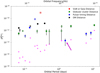Fig. 3. Same as Fig. 1, but excluding the fitting line. The magenta star-like points represent the upper limits of the ${\dot{P}}_b^{\dot{m}}$ for every system with ${\dot{P}}_b^{\mathrm{Res}}$ above a 1σ significance, except for one system with a zero DM uncertainty, which is indicated by the magenta arrow.

For the situation in which the pulsar accretes wind from the companion, the second term in Eq. (16) should be considered, which is inversely proportional to the companion mass m_c. In the other situation in which half of the wind is accreted by the pulsar (ṁ_p = − 0.5 ṁ_c) with m_c = 0.08 M_⊙ and m_p = 1.4 M_⊙, the ${\dot{P}}_b^{\dot{m}}$ is about 26 times larger than that in the situation without accretion, which cannot affect the observational ${\dot{P}}_b^{\mathrm{Obs}}$ significantly.

4.2. Possible origins of the correlation

In almost all tidal models, the tidal response F(ω) has a power-law relation with the tidal frequency ω (Ogilvie 2014). Whereas, our result predicts a power-law relation between the tidal response F(ω) and orbital frequency Ω, which requires a power-law relationship between the tidal frequency ω and the orbital frequency Ω, such a correlation implies a relation between the tidal frequency ω and the orbital period, which probably stems from the epoch of dynamical co-evolution of spin and orbit.

For typical binaries containing a pulsar with a mass of m_p = 1.48 M_⊙ and a WD companion with a mass of m_c = 0.2 M_⊙, the ${\dot{P}}_b^{\mathrm{Tide}}$ can be equivalent to the ${\dot{P}}_b^{\mathrm{GW}}$ originating in GW radiation at a critical period of P_c = 0.077 day, where the ${\dot{P}}_b^{\mathrm{Tide}}$ was calculated by the power law $K=\alpha P_b^{\beta }$ with the fitting result of the first line in the Table 3. For binaries of orbital period P_b > P_c, the tidal interaction determines the change in the orbital period; and for binaries with an orbital period of P_b < P_c, the gravitational radiation is dominant.

Consequently, tidal dissipation is responsible for the variation in the orbital period of the binaries with an orbital period of P_b ≈ 1 day. Even in such a case, the tidal-induced orbital change is only Ṗ_b = 2 × 10⁻¹²ss⁻¹, which is so small that it takes too long for a binary pulsar to evolve from a long orbital period to a short one. Therefore, the scenario of co-evolution can be ruled out.

Such a correlation between the tidal and orbital frequency can originate in the early formation of the pulsar binary, that is, the recycled stage of a millisecond pulsar binary. Interestingly, all systems of pulsar binaries with a WD companion are millisecond pulsar binaries, which are supposed to have experienced a spin-up stage by accelerating the giant companion, the progenitor of the WD. The accretion of NS through mass transfer results in a wider orbit and reduced envelope of the giant star. As the acceleration comes to a halt, the relics of the giant become a naked core, which is the WD companion.

Theoretically, the property of a remnant WD and orbit can be determined by the initial binary status before the recycled stage. Therefore, a correlation between the physical property of a companion and orbital period in a remnant binary is reasonable. For example, Rappaport reported that the mass of a WD is correlated with the orbital period (Rappaport et al. 1995). Thus the spin of the companion may correlate with the orbital period.

The progenitor of a companion is usually thought to be synchronized with the orbit during the accretion phase. However, the WD rotates faster than its progenitor giant. Bassa considered a possibility that the envelope had contracted to form the WD after mass transfer (Bassa et al. 2006a). The conservation of angular momentum increases spin and gives 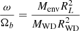$\frac{\omega }{{\mathrm{\Omega }}_b}=\frac{M_{\mathrm{env}}{R}_L^2}{M_{\mathrm{WD}}{R}_{\mathrm{WD}}^2}$, where M_env and R_L is the mass of the envelope and radius of the Roche-lobe, respectively. This scenario leads to the correlation between companion spin and the orbital period. However, it can only align the spin and the orbit, as well as produce a positive ${\dot{P}}_b^{\mathrm{Tide}}$, whereas the negative ${\dot{P}}_b^{\mathrm{Tide}}$ corresponding to the opposite spin and orbital direction cannot be explained in this situation.

The negative ${\dot{P}}_b^{\mathrm{Tide}}$ represents the negative tidal frequency, which means the spin frequency is either smaller than the orbital frequency in the same direction or an arbitrary value in the opposite direction. In almost all WD-MSP binaries, the spin is larger than the orbital frequency in the dynamical tidal model, so the negative ${\dot{P}}_b^{\mathrm{Tide}}$ represents the fast rotation of a companion in the opposite direction as the orbital motion. If the progenitor of a companion has not been synchronized with the orbit and if it has an opposite rotational direction as the orbit, the WD can rotate rapidly in the opposite direction as the orbit.

The tidal dissipation can also affect the evolution of the spin-orbit misalignment angle θ. Lai found that the dumping of the inertial waves in the convective envelope can produce an extra tidal torque to change the spin-orbit inclination misalignment angle θ (Lai 2012), which evolves toward 0 when cos θ < 0 and π when cos θ > 0 if the orbital angular momentum is much larger than the spin angular momentum. In the case that the direction of the companion spin was isotropic in the early stage of the binary and that it has been fully evolved in the recycled stage, then the spin-orbit misalignment angle θ can be either 0 or π, both of which having the same likelihood; this corresponds the distribution of the half negative and half positive ${\dot{P}}_b^{\mathrm{Tide}}$, which is consistent with our expectation.

Now the fast rotation of the companion in both aligned and misaligned situations can be produced, but the origin of the correlation between the companion spin and orbital period remains unknown. Even so, the spin evolution of the companion at the recycled stage is the most probable way to produce such a relation. If the specific relation between the companion spin and orbital period through the recycled process can be understood by other means, the tidal model of WD will be further constrained.

5. Conclusions

There usually are two situations considered in the literature: one is that the companion star is already synchronized with orbit, and the other is that the tidal dissipation on the WD is inefficient. Thus the existence of tidal dissipation in pulsar binaries with the WD companion has long been neglected. Fuller’s study on the dynamical tide of the WD (Fuller & Lai 2012) predicts a more efficient tidal dissipation than viscosity turbulent in Zahn’s equilibrium tidal model (Zahn 1989). On the other hand, the time interval between the recycled stage to the present day is difficult to estimate, and it is not possible to guarantee that the companion has been synchronized with the orbit. Therefore, it is too early to exclude the effect of tidal dissipation from the timing of these pulsar binaries.

After counting out the three normal effects, the residual term ${\dot{P}}_b^{\mathrm{Res}}$ displays signs of being half positive and half negative, which is compatible with the scenario of the tidal effect. We further found that the dynamical tide on the WD can be efficient enough to account for the residual term ${\dot{P}}_b^{\mathrm{Res}}$ of all PSR-WD binaries. For the PSR-MS binary, the Love number of the MS companion of PSR J1227-4853 can be constrained as $k_2=0.{177}_{-0.058}^{+0.098}$, which is a reasonable value for the MS. This supports the possibility of tidal dissipation in the PSR-MS system. Therefore, tidal dissipation should not be ignored in the orbital decay Ṗ_b.

Furthermore, a weak correlation between the tidal parameter and orbital period exhibits a potential relation between the tidal frequency and orbital frequency. As all of the systems are millisecond pulsar binaries, this suggests that such a correlation likely originates from the recycled stage of millisecond pulsar binaries.

Investigation of the tidal dissipation on pulsar binaries is of importance in three aspects. First, it indicates that tidal dissipation also contributes to the first derivative of the orbital period of pulsar binaries, so that fundamental physics such as gravitational radiation of a binary pulsar should be extracted after counting it out. Second, it shows that the interior of the companion stars can be investigated through the precise pulsar timing of these pulsar binaries, which provides a useful complement to previous methods, such as spectroscopy, light curves, eclipse, and asteroseismology. Third, the derived correlation between the tidal and orbital frequency suggests that tidal dissipation may play an important role in the recycled stage of a millisecond pulsar binary.

Acknowledgments

This work is supported by the Ministry of Science and Technology of the People’s Republic of China (2020SKA0120300).

References

Appendix A: Collected Data

All Tables

All Figures

Fig. 1. Relationship between $|{\dot{P}}_b^{\mathrm{Res}}|$ and orbital period Pb in logarithmic coordinates. Only the systems with ${\dot{P}}_b^{\mathrm{Res}}$ in 1σ significance are shown. Different colors represent the binaries of the different ways of the distance measurements1. The solid symbols denote systems with positive ${\dot{P}}_b^{\mathrm{Res}}$ and the hollow ones represent sources with negative ${\dot{P}}_b^{\mathrm{Res}}$. The line is the fitting by the power law relation of systems with a WD companion.

In the text

	Fig. 2. Relationship between K and orbital period Pb in logarithmic coordinates. Only systems with ${\dot{P}}_b^{\mathrm{Res}}$ above a 1σ significance are shown. The meaning of the point style is the same as in Fig. 1.
In the text

	Fig. 3. Same as Fig. 1, but excluding the fitting line. The magenta star-like points represent the upper limits of the ${\dot{P}}_b^{\dot{m}}$ for every system with ${\dot{P}}_b^{\mathrm{Res}}$ above a 1σ significance, except for one system with a zero DM uncertainty, which is indicated by the magenta arrow.
In the text

References

- Andronov, I., & Yavorskij, Y. B. 1990, Contrib. Astron. Obs. Skalnate Pleso, 20, 155 [NASA ADS] [Google Scholar]
- Antoniadis, J., Freire, P. C., Wex, N., et al. 2013, Science, 340, 1233232 [Google Scholar]
- Applegate, J. H., & Shaham, J. 1994, ApJ, 436, 312 [NASA ADS] [CrossRef] [Google Scholar]
- Archibald, A. M., Kaspi, V. M., Hessels, J. W., et al. 2013, ArXiv e-prints [arXiv:1311.5161] [Google Scholar]
- Arzoumanian, Z., Fruchter, A., & Taylor, J. 1993, ApJ, 426, L85 [Google Scholar]
- Arzoumanian, Z., Brazier, A., Burke-Spolaor, S., et al. 2018, ApJS, 235, 37 [CrossRef] [Google Scholar]
- Bassa, C., Van Kerkwijk, M., Koester, D., & Verbunt, F. 2006a, A&A, 456, 295 [NASA ADS] [CrossRef] [EDP Sciences] [Google Scholar]
- Bassa, C., Van Kerkwijk, M., & Kulkarni, S. 2006b, A&A, 450, 295 [NASA ADS] [CrossRef] [EDP Sciences] [Google Scholar]
- Baumgardt, H., Hilker, M., Sollima, A., & Bellini, A. 2018, MNRAS, 482, 5138 [Google Scholar]
- Bhalerao, V. B., & Kulkarni, S. 2011, ApJ, 737, L1 [NASA ADS] [CrossRef] [Google Scholar]
- Bogdanov, S., Archibald, A. M., Bassa, C., et al. 2015, ApJ, 806, 148 [NASA ADS] [CrossRef] [Google Scholar]
- Cadelano, M., Pallanca, C., Ferraro, F., et al. 2015, ApJ, 812, 63 [NASA ADS] [CrossRef] [Google Scholar]
- Cognard, I., Freire, P. C., Guillemot, L., et al. 2017, ApJ, 844, 128 [NASA ADS] [CrossRef] [Google Scholar]
- de Martino, D., Casares, J., Mason, E., et al. 2014, MNRAS, 444, 3004 [Google Scholar]
- Deller, A., Archibald, A., Brisken, W., et al. 2012, ApJ, 756, L25 [NASA ADS] [CrossRef] [Google Scholar]
- Deller, A., Boyles, J., Lorimer, D., et al. 2013, ApJ, 770, 145 [NASA ADS] [CrossRef] [Google Scholar]
- Demircan, O., & Kahraman, G. 1991, Ap&SS, 181, 313 [Google Scholar]
- Desvignes, G., Caballero, R., Lentati, L., et al. 2016, MNRAS, 458, 3341 [NASA ADS] [CrossRef] [Google Scholar]
- Freire, P. C., Hessels, J. W., Nice, D. J., et al. 2005, ApJ, 621, 959 [NASA ADS] [CrossRef] [Google Scholar]
- Freire, P. C., Wex, N., Esposito-Farese, G., et al. 2012, MNRAS, 423, 3328 [NASA ADS] [CrossRef] [Google Scholar]
- Freire, P., Ridolfi, A., Kramer, M., et al. 2017, MNRAS, 471, 857 [NASA ADS] [CrossRef] [Google Scholar]
- Fuller, J., & Lai, D. 2012, MNRAS, 421, 426 [NASA ADS] [Google Scholar]
- Fuller, J., & Lai, D. 2013, MNRAS, 430, 274 [NASA ADS] [CrossRef] [Google Scholar]
- Gaia Collaboration 2018, VizieR Online Data Catalog: I/345 [Google Scholar]
- Goupil, M.-J., & Zahn, J.-P. 2008, Eur. Astron. Soc. Pub. Ser., 29, 67 [Google Scholar]
- Lai, D. 2012, MNRAS, 423, 486 [NASA ADS] [CrossRef] [Google Scholar]
- Lorimer, D. R. 2008, Liv. Rev. Rel., 11, 8 [Google Scholar]
- Lynch, R. S., Freire, P. C., Ransom, S. M., & Jacoby, B. A. 2012, ApJ, 745, 109 [NASA ADS] [CrossRef] [Google Scholar]
- Manchester, R. N., Hobbs, G. B., Teoh, A., & Hobbs, M. 2005, ApJ, 129, 1993 [Google Scholar]
- McMillan, P. J. 2017, MNRAS, 465, 76 [NASA ADS] [CrossRef] [Google Scholar]
- Ogilvie, G. I. 2014, ARA&A, 52, 171 [Google Scholar]
- Özel, F., Psaltis, D., Narayan, R., & Villarreal, A. S. 2012, ApJ, 757, 55 [CrossRef] [Google Scholar]
- Pallanca, C., Ransom, S., Ferraro, F., et al. 2014, ApJ, 795, 29 [NASA ADS] [CrossRef] [Google Scholar]
- Pathak, D., & Bagchi, M. 2019, ArXiv e-prints [arXiv:1905.01159] [Google Scholar]
- Rappaport, S., Podsiadlowski, P., Joss, P., Di Stefano, R., & Han, Z. 1995, MNRAS, 273, 731 [NASA ADS] [CrossRef] [Google Scholar]
- Reardon, D., Hobbs, G., Coles, W., et al. 2015, MNRAS, 455, 1751 [Google Scholar]
- Ridolfi, A., Freire, P., Torne, P., et al. 2016, MNRAS, 462, 2918 [NASA ADS] [CrossRef] [Google Scholar]
- Roy, J., Ray, P. S., Bhattacharyya, B., et al. 2015, ApJ, 800, L12 [Google Scholar]
- Shklovskii, I. 1970, Sov. Astron., 13, 562 [NASA ADS] [Google Scholar]
- Stovall, K., Allen, B., Bogdanov, S., et al. 2016, ApJ, 833, 192 [NASA ADS] [CrossRef] [Google Scholar]
- Tout, C. A., & Hall, D. S. 1991, MNRAS, 253, 9 [NASA ADS] [CrossRef] [Google Scholar]
- Unglaub, K. 2008, A&A, 486, 923 [NASA ADS] [CrossRef] [EDP Sciences] [Google Scholar]
- van Kerkwijk, M. H., Bassa, C., Jacoby, B., & Jonker, P. 2005, in Binary Radio Pulsars, Proceedings of the conference, 11-17 January, 2004, Aspen, Colorado, USA, eds. F. A. Rasio, & I. H. Stairs, (San Francisco: Astronomical Society of the Pacific) ASP Conf. Ser., 328, 357 [Google Scholar]
- Yao, J., Manchester, R., & Wang, N. 2017, ApJ, 835, 29 [NASA ADS] [CrossRef] [Google Scholar]
- Zahn, J.-P. 1989, A&A, 220, 112 [NASA ADS] [Google Scholar]
- Zhang, X., Zhao, W., Liu, T., et al. 2019, ApJ, 874, 121 [NASA ADS] [CrossRef] [Google Scholar]
- Zhu, W., Desvignes, G., Wex, N., et al. 2018, MNRAS, 482, 3249 [Google Scholar]