| Issue |
A&A
Volume 661, May 2022
|
|
|---|---|---|
| Article Number | A110 | |
| Number of page(s) | 9 | |
| Section | Stellar atmospheres | |
| DOI | https://doi.org/10.1051/0004-6361/202243041 | |
| Published online | 24 May 2022 | |
Emission properties and bidrifting subpulses in pulsar PSR J0815+0939
1
Xinjiang Astronomical Observatory, Chinese Academy of Sciences,
150 Science 1-Street, Urumqi,
Xinjiang
830011,
PR China
e-mail: This email address is being protected from spambots. You need JavaScript enabled to view it.
2
Key laboratory of Radio Astronomy, Chinese Academy of Sciences,
Nanjing
210008,
PR China
3
SIfA, School of Physics, University of Sydney,
Sydney,
NSW
2006,
Australia
Received:
4
January
2022
Accepted:
17
March
2022
Abstract
Context. We investigate the properties of the emission region in PSR J0815+0939 as revealed by the bidrifting subpulses.
Aims. We identify the emission properties as implied by different states of emission, including the charge density and the subpulse number on the carousel, in association with the different subpulse drift properties in bidrifting.
Methods. The investigation is based on the rotating carousel, incorporating the model for obliquely rotating pulsar magnetospheres of multiple emission states. For the subpulse drift velocity given by the electric drift, the latter changes as the emission state changes, resulting in the observed different drift-bands.
Results. Our results show that observable emission of this pulsar comes from two rotating carousels. The carousel at higher height is occupied by two different emission states. We find that the subpulse drift direction is different for emission coming either from different emission states on the same carousel or from similar emission states, but located on different carousels. We consider that establishing the subpulse number on a carousel may involve a mechanism that is not a function of the age or the obliquity angle of the pulsar. We discuss that bidrifting may be a common phenomenon, but its detection requires particular emission characteristics of the pulsar. We relate different subpulse drift modes in bidrifting with drifting subpulses of time-dependent drift rates, and speculate that they may be two manifestations of the same underlying mechanism.
Key words: pulsars: general / stars: neutron / radiation mechanisms: non-thermal
© ESO 2022
1 Introduction
Early observations of the single-pulse emission from PSR J0815+0939 revealed unusual evolutionary features that are shown as subpulse drifting along four distinct drift-bands in different profile components, with the drift direction of each in opposing sense on either side of the fiducial plane (McLaughlin et al. 2004; Champion et al. 2005). Called bidrifting (Qiao et al. 2004; Wright & Weltevrede 2017), the phenomenon has provided a distinctive way to explore pulsar radio emission (Qiao et al. 2004; Szary & van Leeuwen 2017). In traditional models, drifting subpulses are described as the systematic motion of subpulses across the profile window in a sequence of pulses. The explanation involves assuming that the emitting locations are confined to discrete subbeams that are placed evenly on carousels rotating about the magnetic axis under the E × B drift (Ruderman & Sutherland 1975; Deshpande & Rankin 1999, 2001). In this rotating-carousel model, the subpulses appear to drift as the subbeams rotate relative to corotation through the fixed line of sight. The model offers an important interpretation for the subpulse drift properties described in terms of distinct values of P2, the separation between two consecutive subpulses in a single pulse, and P3, the time interval for the repeating drift pattern, with the drift rate given by P2/P3 (Manchester & Taylor 1977). It also provides a means for deriving several essential pulsar parameters. This includes the viewing angle, ζ, between the line of sight and the rotation axis, and the obliquity angle, α, between the magnetic and the rotation axes. Furthermore, the assumption of emission from well-organized subbeams on a carousel leads to a consistent and constant drift direction for a pulsar. In this regards, the bidrifting subpulses in PSR J0815+0939 are ‘traditional’ when the drift-bands are treated separately. This is because the drift properties for each drift-band can also be described by particular values of P2 and P3 based on the carousel model. Since drifting subpulses are linked to the emission properties (Ruderman & Sutherland 1975), bidrifting suggests that different emission properties, corresponding to different emission states in our model, can exist in the emission region and function at the same time. However, questions such as how the emission properties differ across different driftbands, and how the different emission properties are arranged in the emission region are unclear. Therefore, the pulsar provides a unique window to probe the observable radio emission region as revealed by the unusual drifting subpulses.
The purpose of this paper is to explore the different emission properties and their arrangements in the pulsar emission region as revealed by bidrifting subpulses in PSR J0815+0939. Our investigation is based on the rotating carousel, incorporating the model for a pulsar magnetosphere of multiple emission states designated by the parameter y (Melrose & Yuen 2014, 2016; Yuen 2019). A periodic structure of underdense and overdense (subbeams) regions of plasma is assumed to underlie the emission. The structure varies in proportional to cos(mϕb) (Clemens & Rosen 2004; Godoberidze et al. 2005) in azimuthal direction around the magnetic axis, where m is an integer and ϕb is the azimuthal angle, with subscript b signifying the magnetic frame. This is due to a standing wave of a specific spherical harmonic determined by an instability in the magnetosphere (Fung et al. 2006; Pétri 2007). We also assume that the subpulse drift velocity is the flow rate of the emitting plasma, υdr, defined by the electric drift velocity E × B/B2. For an obliquely rotating pulsar magnetosphere with multiple emission states, E is a function of y such that the value of υdr is intermediate between the corotation value due to the (oblique) corotation electric field and that owing to the inductive electric field from a rotating magnetic dipole in vacuum. Therefore, a change in y leads to a change in the drift velocity. The implication of bidrifting is that the value of y varies as a function of ϕb in the magnetic frame (Melrose & Yuen 2016). In this model, observable subpulses are interpreted in terms of emission from the overdense regions (subbeams), corresponding to m emission areas. Subpulse drifting is due to the flow of the emission areas relative to corotation under the influence of the E × B drift in a particular emission state. This gives a carousel-type model with m emission areas. Because emission properties are connected to drifting subpulses, the model provides a unique way to identify the emission states (y) and the subpulse number (m) for known subpulse drift properties. Therefore, the model offers a unified approach to identify the different emission properties and the associated variation in the emission structure across the observable emission region.
Investigation of drifting subpulses usually involves models that assume a plasma-filled magnetosphere in corotation with the star. The simplest form of the corotation model is for an aligned model, first introduced by Goldreich & Julian (1969), in which there is no time dependence, and the electrodynamics reduces to electrostatics. This ignores certain essential electrodynamics, such as that (i) the corotation electric field consists of both a potential and an inductive component (Hones & Bergeson 1965; Melrose & Yuen 2014), whereas the aligned case has no inductive electric field, and (ii) there is no magnetic dipole radiation. Subsequent developments of more detailed models emphasized the aligned case, and the electrostatic assumption was extended to oblique rotators by postulating corotation in the magnetospheric plasma (Scharlemann et al. 1978). An example is the Ruderman & Sutherland (1975) model, which has become the standard model for drifting subpulses. A generalization to an oblique rotator involves ensuring that the parallel electric field (to the magnetic field) is zero and the electric field has the form of E = Ecor – grad V for a particular field line. Here, Ecor is the corotation electric field and V is a potential. A specific model then involves determining the function V on either side of the gap. A complication, compared to an aligned model, is that the potential drop also includes the contribution from the line integral of the inductive field (Melrose & Yuen 2016). In practical terms, the assumption of alignment and the related electrostatic assumption in an obliquely corotating magnetosphere (Fawley et al. 1977; Scharlemann et al. 1978) are important approximations that allow detailed models to be developed. However, a more realistic model must include oblique rotation. The model used in this paper is based on a purely magnetospheric interpretation of emission from discrete areas in terms of a standing wave structure. It incorporates obliquity, and electromagnetic fields induced by a time-dependent rotating magnetic dipole. An intrinsically different feature of our oblique model as compared with an aligned model is the presence of the inductive field. Based on this, a class of synthesized models can be established by combining the minimal model (cf. Sect. 2.1) and the corotation model. Then an oblique form of the corotation model applies to any obliquity angle, which reduces to the special case for an aligned rotator assumed by Goldreich & Julian (1969).
In Sect. 2, we outline the model for the variation in drifting subpulses and the opposite drift directions. In Sect. 3, we present the simulation setup and the results. The emission arrangement as implied by the different emission states is explored in Sect. 4. We discuss a few implications of our results and conclude the paper in Sect. 5. The viewing geometry used in this paper is given in Appendix A.
2 Variation in drifting subpulses
We describe the properties of drifting subpulses using P2 and P3, with the drift rate given by P2/P3. In this section, we summarize the model for varying the two parameters in a pulsar magnetosphere of multiple emission states based on Melrose & Yuen (2014) and Yuen (2019). Most of the analysis in this section is derived from the two papers.
2.1 Flow rate of the plasma
The plasma flow rate is defined by the electric drift, which has the form in our model of
 (1)
(1)
where the dipolar term of the magnetic field is given by
 (2)
(2)
and μ0 is the vacuum permeability. Here, x and p are the position vector from the stellar center and the rotating magnetic dipole, respectively, and r = |x|. The electric field has the form (Melrose & Yuen 2014)
 (3)
(3)
where the electric field relevant to the corotation charge density is denoted by Epot = − grad Φcor, and b represents the unit vector along the dipolar magnetic field lines. The Eind is the inductive electric field due to the obliquely rotating dipole in vacuum, given by
 (4)
(4)
where Eind possesses components parallel, Eind‖, and perpendicular, Eind⊥, to the magnetic field (Melrose & Yuen 2012).
An emission state is represented by a particular value in the parameter y between zero and one. The case of y = 0 corresponds to the state described in the corotation model (Goldreich & Julian 1969), and E is the corotation electric field given by Ecor = −(ω⋆ × x) × B, where ω⋆ is the angular velocity of the star. The drift velocity is then given by υdr = υcor = Ecor × B/B2, resulting in corotation in the region with the star. The minimal model, denoted by y = 1, represents a state in which Eind‖ is screened by a charge density that produces an electric field Emin = −Eind‖, while Eind⊥ possesses the same value as in the vacuum-dipole model (Melrose & Yuen 2014). This implies a drift velocity given by υdr = Eind⊥ × B/B2. For an oblique rotator and 0 < y < 1, Eq. (1) gives υdr, which is a fraction y of the value in υcor and (1 − y) of the drift velocity due to Eind⊥ in the minimal model. Dividing υdr by r gives the angular velocity, ωdr, in the form
 (5)
(5)
For an obliquely rotating magnetosphere, the allowed emission states (y) are of the form defined by Eq. (5).
The divergence of Emin implies a charge density in the minimal model, which has the form given by (Melrose & Yuen 2014)
 (6)
(6)
where ε0 is the vacuum permittivity. For each intermediate emission state, a charge density is required to screen the electric field along the magnetic field lines. For an oblique rotator, the screening charge density is designated by (Melrose & Yuen 2014)
 (7)
(7)
where
 (8)
(8)
is the corotation charge density (Goldreich & Julian 1969).
2.2 Visible emission region
The quantities described in Sect. 2.1 can be determined uniquely at given coordinates in an emission geometry for known ζ and α. We assume a geometry (see Appendix A) in which emission at the source point is directed along the local dipolar magnetic field line (Hibschman & Arons 2001) and the emission arises only within the open-field region (Cordes 1978; Kijak & Gil 2003). For given ζ and α, an explicit solution for the angular location of the point where emission is visible is given by the polar and azimuthal angles in the magnetic frame, (θbV, ϕbV), as a function of the rotational phase of the pulsar, ψ, in Eq. (A.5). In the observer’s frame, the visible point is expressed in terms of (θV,ϕV) relative to the rotation axis using Eqs. (A.6) and (A.7). For α ≠ 0, the visible point moves at an angular speed, ωV, that varies as a function of ψ with the lowest speed dependent on α. The visible point traces a path as the pulsar rotates and forms a closed curve after one pulsar rotation, referred to here as the trajectory of the visible point. The size and shape of a trajectory is dependent on ζ and α, which is generally not circular and may or may not enclose the magnetic axis. Figure 1 shows four examples of the trajectory of the visible point in the magnetic frame using {ζ, α} = (0°, 8°) (red), (10°, 25°) (blue), (40°, 35°) (green), and (30°, 40°) (black). Only trajectories in red and green enclose the magnetic pole, with the former also centered at the origin. An open-field region of height at 0.02rL, and assuming α = 0°, is shown as the dotted gray circle in Fig. 1. The dependence of the visible point on height, r ≥ rV, follows from the assumption that emission comes only from within the open-field region, with rV given by Eq. (A.8). Three trajectories cut the open-field region, with the trajectory in red entirely within the region. The exception is the trajectory in blue, which lies outside of the open-field region, implying that emission is not visible from any point on the trajectory.
Drifting subpulses in many pulsars are interpreted in terms of emission from favored locations that are distributed periodically around the magnetic axis forming structures that flow relative to corotation. In the carousel model (Deshpande & Rankin 1999), these structures are not fixed, and subpulses are interpreted as emission from plasma columns distributed uniformly around the magnetic axis. A simple interpretation of these plasma columns is in terms of antinodes (or nodes) due to a wave that grows preferentially at a specific spherical harmonic (Clemens & Rosen 2004; Godoberidze et al. 2005) generated by a large-scale instability in the magnetosphere (Arons 1981; Jones 1984; Kazbegi et al. 1991). This gives rise to a periodic pattern of overdense (antinodes) and underdense (nodes) plasma that is proportional to cos(mϕb), corresponding to m antinodes. Emission from subpulses is then assumed coming from m discrete emission areas that are confined to regions of overdense plasma (antinodes). This describes a carousel-type model with m nodes and antinodes in a pattern that varies proportional to cos(mφb) around the magnetic axis. However, the distribution of each of the m areas in r and θb is unknown. Here, we assume that the location of the discrete areas is independent of polar angle and locally independent of r, and each has the same diameter (Gil & Sendyk 2000). This results in alignment of the discrete areas along the radial direction, producing a structure of radial spokes when projected onto a surface of constant r, as shown in Fig. 1. The trajectory of the visible point then cuts the spokes at different θb = θbV and ϕb = ϕbV, whose values are dependent on ζ, α. From Fig. 1, visibility requires emission to come from a discrete area (antinode) that lies on the trajectory whose location must lie inside the open-field region, and we refer to this discrete emission area as the emission spot. Assuming that the discrete emission areas (emission spots) are fixed to the magnetospheric plasma implies that the emission spots have the angular velocity of the plasma given by Eq. (5). Therefore, two parameters are relevant to drifting subpulses in this model: (i) the flow rate (ωdr) of the discrete emission areas (antinodes), and (ii) the angular speed of the visible point (ωV ≠ 0), with both being determined along the trajectory of the visible point. This also indicates that both noncorotating plasma and the trajectory of the visible point can affect the observed emission pattern. In general, a trajectory of the visible point is not centered at the magnetic pole, which also implies that the apparent flow and rotation of emission spots are not centered at the magnetic axis.
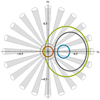 |
Fig. 1 Four trajectories of the visible point in the magnetic frame using different combinations of (ζ, α). The magnetic pole is located at the origin. An arrangement of 20 radial spokes is also shown in gray circular cones that are located around and radiating from the magnetic pole. |
2.3 Subpulse drifting
The apparent ωdr is the projected components onto the trajectory of the visible point at locations defined by the latter. In addition, since ωV is a function of ψ, the apparent motion of a subpulse would depend not only on the relative velocity, but also on the particular emission spot (m). This implies that P2 represents the time between the visible point coinciding with neighboring emission spots. When the motion of the visible point (ωV = 0) is ignored, m emission spots will pass through the line of sight in the time given by 2π/ωdr that it takes for the plasma to complete one rotation. The separation of consecutive emission spots would then be observed with an interval given by 2π/mωdr. This interval is modified when taking ωV into account, giving (Yuen 2019)
 (9)
(9)
or ω⋆P2 in radians. Both the visible point and the antinodes are rotating at different angular velocities, and both are different from ω⋆. For a plasma-filled magnetosphere in the traditional picture (Goldreich & Julian 1969; Ruderman & Sutherland 1975), the delay between identical repeating patterns (P3) is dependent on ωdr − ωcor, where ωdr = ωcor (at y = 0) signifies a stationary pattern that is unchanged in a sequence of pulses. The assumption that an observer sees the same momentary drift pattern suggests that ωV is irrelevant. Then, a difference between ωdr and ωcor results in a slowly changing pattern in consecutive pulses that repeats after several pulsar rotations. This gives (Yuen 2019)
 (10)
(10)
The subpulse drift rate is then given by
 (11)
(11)
From Eqs. (9)–(11), P2, P3, and the associated drift rate will change with a change in m or y of a pulsar. Both ωdr and ωcor are determined on the trajectory of the visible point, and these are the components that we refer to in the rest of the paper. Subpulses drift because ωdr ≠ ωcor, which gives rise to a relative motion between corotation and the flow rate of the emitting plasma along the trajectory of the visible point. This results in observable periodic modulation of subpulses flowing across the profile window. Therefore, drifting subpulses with specific drift properties in P2, P3, and the drift rate can be associated with particular values of y, m, and ρsn, and they are collectively referred to as a subpulse drift mode in this paper.
2.4 Interpretation of the drift direction
The dependence of P3 on ωdr and ωcor implies a progressive change in the longitudinal phase of an emission spot for any differences between the values of the two parameters. For a small deviation (ωdr ≠ ωcor), the change is given by δϕ = (ωdr − ωcor)P1 between two consecutive pulses. Here, P1 = 2π/ω⋆ is the rotation period of the star. For δϕ > 0, the plasma flow is ahead of corotation, resulting in a forward movement for the emission spots to later longitudinal phases in successive pulses. The tracks traced by the subpulses will appear to lean forward, giving a positive slope. This is interpreted in the conventional notation as positive drifting, with the value of P2 expressed as positive. For δϕ < 0, the plasma falls behind corotation, and an emission spot will move toward earlier longitudinal phases in successive pulses. The drift is in the opposite direction, and the tracks traced by the subpulses will appear to lean backward, giving a negative slope. The drift rate is negative, and the value of P2 is assumed negative in the conventional notation. In either case, the result is a slowly changing pattern that repeats in a sequence of pulses.
For an oblique rotator, ωdr and ωcor are not constants, but vary as a function of pulsar phase, ψ, where ωdr also varies as a function of y, as shown in Fig. 2. It follows that changes in (ωdr - ωcor) are dependent on ψ and y. Consider the curve in red relative to gray (y = 0), with the visible point moving toward more positive ψ. The change in δφ is such that its sign is positive and the value is maximum at ψ = −180°, from where its value begins to decrease as ψ increases and reaches zero at about ψ = −55°. It then increases, with the sign reversed, and reaches zero again at ψ = 55°. After this, the sign of δϕ returns to positive. Its value increases and reaches maximum again at ψ = 180°. In general, the value of δϕ increases as y increases for a given ψ.
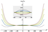 |
Fig. 2 Variation in ωdr in units of ω⋆ along the trajectory of the visible point using ζ = 10° and α = 25° for y = 0.2 (blue), 0.4 (green), 0.6 (yellow), and 0.8 (red). The case for corotation (y = 0) is indicated by the curve in gray. The inset is a zoom-in for the range of ψ ≤ |60°|. |
3 Simulation
Early observations of PSR J0815+0939 showed that drifting subpulses were present in all four components of the integrated profile, with the drift direction reversed on either side of the fiducial plane (McLaughlin et al. 2004; Champion et al. 2005). Recent investigation revealed that an opposite drift direction occurs only in the second component (Szary & van Leeuwen 2017). We adopt the latter in the following analysis. For easy reference, the properties of the bidrifting subpulses are reproduced in sector I under the label Observation in Table 1.
3.1 Setup
Our simulation setup begins with the determination for the width of each component region that contains drifting subpulses. There are four component regions, referred to as A, B, C, and D, with the width of each given by Szary & van Leeuwen (2017). Since α is unknown for this pulsar, different trajectories of the visible point were determined based on α from 1° to 85° in steps of 1°, with an impact parameter β = ζ − α ≤ |5°| under a maximum height of 0.2rL, where rL is the light cylinder radius. We assumed that the rotation direction of the pulsar corresponds to the visible point moving toward more positive ψ. The simulation was then performed along each trajectory of the visible point to search for the values of m and y using Eqs. (9)–(11), which give the drift rate, P3, and the associated drift direction in each region within the respective observed uncertainty. Specifically, the values of ωdr and ωcor were determined for all m := [1, 45], in steps of 1, and y := [0, 1], in steps of 10−4, along a trajectory of the visible point over the range of ψ (equivalent to the width of each region) with a division of 0.1°. The value of ωV for a given ζ and α was evaluated along the trajectory for each ψ in steps of 0.1° using Eq. (A.9) with Eq. (A.5). The drift rate was determined first. Then for every simulated drift rate that matched the observed value for a component region, the same combination of ωdr and ωcor was used to calculate the value of P3 and the associated sign. When the matching values were found, the results were weighted based on the uncertainty in the drift rate. For example, a simulated value that falls within the uncertainty of the observed value receives a weight proportional to 1 − |x|, where x is the interval between the observed and simulated values, normalized by the maximum reported uncertainty. It follows that a result that matches the observed value more closely will receive more weight. Then, each simulated value from the same calculation received the same weight. At the end of the whole simulation, a weighted average was determined for each of the parameters.
Details of the bidrifting subpulses in PSR J0815+0939, including the observed drift properties and the associated width for each component region, are given in sector I (Szary & van Leeuwen 2017).
3.2 Results
The results of simulation are shown in sectors II and III in Table 1. Sector II gives the values for P3 and the drift rate obtained from our simulation for the drifting subpulses in each component region. In our model, the subpulses would appear to drift in opposite direction when (ωdr − ωcor) changes sign. For regions A, B, C, and D, the mean values of ωdr/ωcor are 0.998, 1.003, 0.999, 0.998, respectively. This indicates that subpulses drift in the same direction in regions A, C, and D, which is negative, in opposite to that in region B, which has a positive drift. In Table 1 we reserve the sign for the drift direction in P2 to conform with the traditional convention. When we decided whether a simulated value was consistent with an observed value, we compared the range of their uncertainties. If the uncertainties overlapped, the two values were considered consistent. This requirement was met by all simulated values of P3 and drift rates. In addition, the simulated P3 values for the four components are consistent with each other within their uncertainties. The average simulated P3 value is (17.3 ± 5.2)P1, which agrees with the observed value within the uncertainty. The prediction for α is 8° ± 2°, which is consistent with that assumed by Szary & van Leeuwen (2017). We find that the fiducial plane is located at ψ = −86° on average.
The values of m and y obtained from our simulation based on the drifting subpulses in each of the component regions are shown in sector III. The y value in region A is different from that in regions B, C, and D, suggesting that the emission region contains different emission states. While the value of y is similar within the uncertainty for regions B, C, and D, it shows a preference for a higher value in region C. The average value of y is 0.003 ± 0.002, which is low, consistent with the low drift rates, indicating that the plasma flow deviates from corotation. The number of emission spots on the carousel, as revealed by the value of m, shows variation across the component regions. We find that the value of m as predicted from the drifting subpulses in regions A and B is similar within the uncertainty, but a lower m value is predicted for regions C and D. The prediction of a similar y value for regions B and D, regardless of m, suggests that the number of subpulses on a carousel is not related to the emission state in the emission region. The average value of m is 18 ± 6, which is consistent with 20 predicted by Mitra & Rankin (2008).
It is straightforward to determine the overall charge density for each component region using Eq. (7) when the value of y is known for that region. The results are expressed in the units of ρGJ and are shown in the third column in sector III. The value of ρsn(ρGJ) is not unity, indicating that the charge density deviates from the Goldreich–Julian value in all component regions. Our results suggest that the charge density is evenly spread across all regions within the uncertainty, with a preference for a higher value in region A.
4 Emission arrangement and emission state
The arrangement of the rotating carousels in an emission region and its relation to r is unknown in the traditional models. This is partly due to the poor determination for the source height r of a visible emission. The latter is usually estimated based either on (i) relativistic phase shift in the components of an asymmetric pulse profile (Dyks et al. 2004), or (ii) geometry, in which the source is assumed to be located on the last closed field lines (Kijak & Gil 2003). We adopted the second approach to estimate the emission height as described by Eq. (A.8). For all the values in the parameter space for ζ and α (i.e., α = 8° ± 2° and β ≤ |5°|), the trajectory begins at a higher height in region A, then decreases as it traverses the open region, and reaches the lowest height at the exit in region D. Figure 3 shows an example for the variation in height along the trajectory, using ζ = 10° and α = 8°, across the profile defined by the visible emission bounded by the two vertical dashed lines in purple. From Eq. (A.5), ϕbV decreases as ψ increases, and hence the trajectory advances from right to left in the figure. The average minimum height is (0.016 ± 0.001)rL.
Our assumption of an even distribution of antinodes around the magnetic axis implies that the subbeams are spread uniformly on a carousel. Some investigations also predicted different subpulse numbers for different pulsars (Gil et al. 2003; Esamdin et al. 2005; Smits et al. 2007; Mitra & Rankin 2008), which implies that the value of m is not a fixed number for different carousels. For PSR J0815+0939, it implies that the observable emission from the neighboring regions A and B, both with similar predicted m value, comes from the same carousel. Similarly, for regions C and D, it means that the emission spots from the two regions are located on another carousel. The locations for the two carousels1 are illustrated in Fig. 3 based on the same values of ζ and α. The average heights for the upper and lower carousels are at (0.025 ± 0.002)rL and (0.009 ± 0.001)rL, respectively. The trajectory cuts the two carousels in the way that it traverses the carousel at higher height in regions A and B, followed by the carousel at lower height in regions C and D. We note that the start of the lower carousel and the end of the upper carousel are uncertain, and they were chosen at the left and right boundaries of the profile, respectively, in the figure. An observer then sees emission only from the higher carousel (but not from the lower carousel) that forms the first half of the profile. As the pulsar rotates, emission is observable from the lower carousel (but not from the higher carousel) that forms the second half of the profile.
For different values of m, Eqs. (9) and (10) suggest that the subpulse drift properties, and hence the associated emission properties, will also be different between the two carousels. From the values of y, the carousel in regions C and D is occupied by a similar emission state. However, the part of the carousel that forms the visible region A has an emission state that is different from that in region B. Since the variation in height is predicted from high to low across regions from A to D, the carousel located at higher height is occupied by (at least) two different emission states. This suggests a dependence on r of the emission properties on the carousels, with more different emission states at higher height in this pulsar. It follows that the different subpulse drift directions between regions A and B and between B and C are due to different causes. In the former, the two different subpulse drift modes with opposite drift direction correspond to emission from two different emission states, each covering a specific range of azimuthal angle around the magnetic axis. However, the different drift modes between regions B and C is the result of the trajectory of the visible point traversing two carousels over the parts with different emission properties. The different subpulse drift modes, but of the same drift direction, between regions C and D of similar emission state are due to variation in ωdr and ωcor across different ranges of longitudinal phases. From the changes in the values of m and y across regions of different heights, it appears that some kind of frequency-to-radius mapping applies in this pulsar.
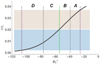 |
Fig. 3 Magnetic frame, showing the variation in height across the visible emission region bounded by two vertical dashed lines in purple. The fiducial point is indicated by the vertical dashed line in green. The component regions are separated by the vertical dashed lines. The asymmetric coverage of ϕb about the fiducial plane is due the variation in the motion of the visible point from high to low as ϕb decreases. Two zones (brown and blue) representing the two carousels are shown as well. The traversal of the trajectory is toward more negative ϕb, cutting first the carousel at higher height (brown) and then the carousel at lower height (blue). |
5 Discussion and conclusions
We have investigated the properties of the emission region in PSR J0815+0939 based on the rotating-carousel model in a pulsar magnetosphere of multiple emission states. A quantitative definition of an emission state is through the plasma flow, ωdr, in the magnetosphere, which is parameterized by 0 ≤ y ≤ 1, with the inferred emission state corresponding to a particular value in y. In our model, the observable drift of subpulses is due to the plasma flow, ωdr, induced by the E × B drift in an emission state, designated by the parameter y, which deviates from corotation, and different emission states (y) imply different ωdr. We interpret the subpulses as emission from m discrete spots that are arranged in azimuth around the magnetic axis. The model allows the identification of the emission state (y) and the subpulse number (m) in association with the drifting subpulses in a component region, which are referred to as a subpulse drift mode. Our results show that different subpulse drift modes can be associated with particular values of y and m in the emission region. When we assume that the subpulses are evenly distributed around a carousel, the different subpulse numbers between regions AB and CD suggest that observable emission comes from two carousels each locates at different heights. We find that changes in the drift direction are due to emission coming either from different emission states on the same carousel or from different carousels of differing emission properties.
It has been shown that variation in the drift rate can arise given the right alias orders (van Leeuwen et al. 2003; McSweeney et al. 2019). Aliasing in PSR J0815+0939 was considered by Szary & van Leeuwen (2017), and they concluded that the effect did not produce the correct drift-rate and the drift reversal in component region B. In our model, the behavior of drifting subpulses is related to the number of emission spots (m) and the plasma flow (ωdr), where the latter is related to y. Given that the simulated P3 values are similar across the four components, the results displayed in Table 1 are perhaps an aliased pattern of a single carousel. However, if this is case, the variation in m across the components would imply a nonuniform distribution of emission spots on the carousel. This is inconsistent with the observation by Deshpande & Rankin (1999)2, who clearly suggested that the emission spots are of equal size and uniformly distributed equidistantly on a carousel (Gil & Sendyk 2000). A related point is that aliasing is expected to apply to the whole carousel system (Janssen & van Leeuwen 2004; Rankin et al. 2013; Szary & van Leeuwen 2017), which implies that this uniformity on a carousel should persevere for different alias orders (Gupta et al. 2004; Bhattacharyya et al. 2009). This is consistent with the results of Deshpande & Rankin (1999), who took aliasing into account. Changes in the number of the emission areas (m) on a single carousel due to aliasing have also been proposed to account for drifting subpulses with different drift modes (Rankin et al. 2013; McSweeney et al. 2019). However, each change is for a unique epoch and to the whole carousel, which implies that the distribution of the emission areas remains uniform on the carousel at all times. Thus, the changes in m as predicted for PSR J0815+0939 across different longitudinal phases may be considered an indication that they are not caused by aliasing. We may still interpret the different m values as different alias orders of an underlying uniform carousel. However, aliasing on individual profile components has not been shown in the literature before (Szary & van Leeuwen 2017), and how to interpret such aliasing is unclear. Therefore, we prefer the interpretation that bidrifting in this pulsar is not likely due to aliasing.
In the context of the Ruderman & Sutherland (1975) model, the potential difference between the pulsar surface and magnetosphere produces a layer near the polar cap called the vacuum gap, where particles are accelerated. The gap discharges in the form of a number of isolated and short-lived sparks, which can be interpreted as emitting plasma columns. As mentioned above, the sparks (or emission spots in our case) have been shown to be uniformly distributed on a carousel (Ruderman & Sutherland 1975; Deshpande & Rankin 1999; Gil & Sendyk 2000). This also implies that carousels with a different number of sparks are separated. The prediction of similar m for component regions A and B, but different from that for component regions C and D, implies that the emission spots responsible for emission from the first two regions are located on a carousel different from that for the second two regions. Furthermore, the drift reversal between component regions AB, but not between CD, indicates that the properties of the two carousels are different. The prediction of consistent subpulse drift properties in the Ruderman & Sutherland (1975) model would imply that the two carousels are also likely separated. In addition, the presence of a gap in an obliquely rotating magnetosphere implies that the plasma flow rate below the gap is different from that above the gap (Melrose & Yuen 2014). However, the location and size of the gaps are still not convincingly identified from the related electrodynamics (Bai & Spitkovsky 2010; Melrose & Yuen 2016), but it is plausible that the acceleration and emission regions are colocated (Melrose & Yuen 2016). This implies that emission can come from different heights. From Eq. (A.8), a decreasing height is predicted across the profile from regions A to D. This implies that the two carousels are located at different heights. For radiation emitted tangential to dipolar magnetic field lines, a well-organized emitting region extends radially, and the emission spots can each be associated with a particular magnetic surface of emission. The above leads to the picture of an emission region for PSR J0815+0939 with two concentric radiating carousels located at different heights.
Bidrifting pulsars are rare (Weltevrede et al. 2006). The question is then how the results presented in this paper are relevant to other pulsars with traditional drifting subpulses. Figure 2 shows that variation in δϕ should be common for obliquely rotating magnetospheres with ζ > 0. In general, the variation in δϕ is dependent of both ζ and α and the effect may be small, which means that detection of significant changes in δϕ favors a broad profile window. The latter implies that the open field region needs to be at a sufficient height for a pulsar so that the trajectory traverses it over a wide range of pulsar phase. For PSR J0815+0939, the profile window is 112°, which is relatively wide compare to most ordinary radio pulsars (Maciesiak et al. 2011). Another example of unusual drifting subpulses is that observed in PSR B0826–34. The drifting subpulses are shown to vary as P2 and P3 and the drift direction in both the mainpulse and interpulse varies over profile widths of 94° and 143°, respectively (Esamdin et al. 2005). Variation in |δϕ| is also proportional to the emission state, as shown in Fig. 2. This implies that a detection of this variation is possible even for narrow profiles if emission comes from an emission state that deviates largely from corotation. As discussed in Sect. 4, opposite drift directions may arise from emission that originates from different carousels of differing emission properties and located at different heights. Since most pulsars have narrow profiles, and unless the change in the emission height is large across the profile, emission is likely coming from a single carousel. Assuming uniform properties for a carousel suggests that subpulse drifting would appear traditional for many pulsars. Therefore, our model predicts that bidrifting should be a common phenomenon, but the observation requires specific characteristics of the pulsar. The latter includes (i) a broad profile width, (ii) emission from an emission state with a high y value, and (iii) a strong change in emission height across the profile.
The fact that radio emission is detected from PSR J0815+0939 indicates that the traditional emission mechanism (Ruderman & Sutherland 1975) is functioning in the magnetosphere. A feature of the mechanism is related to the assumption of a relativistic outflow of pair plasma along open field lines in the two-stream instability, implying that radio emission is related to the plasma density (Lyubarskii 1996). The latter involves creation of electron-positron pairs with a multiplicity, λ, that is high enough to screen the accelerating potential in the vacuum gap (Ruderman & Sutherland 1975; Melrose & Yuen 2012). In our model, this implies e(n+ + n−) = λρsn for an emission state, where n± are the number densities for the electrons and positrons. Assuming the same λ for all y means that radio emission is related to ρsn. The proposal of pulse emission coming from a plasma-filled magnetosphere that ceased in a vacuum magnetosphere (Kramer et al. 2006) suggests that pulsar emission, and hence the associated observable emission structure (subpulses), varies with the emitting plasma. This also implies that our assumption for emission areas originating from a periodic structure of plasma is also related to ρsn. It then follows that the values of ρsn and m should be correlated if the traditional emission mechanism is also responsible for the subpulse number on a carousel. However, this is not the case, as shown in Table 1. The variation in y across regions A and B, with a preference for different ρsn, does not correspond to a change in the value of m (within the uncertainty). However, a significant difference in m is seen between regions B and C (or B and D), but with similar y and ρsn in the regions. Another feature of the traditional radio emission mechanism is the prediction that radio emission is correlated with pulsar evolution. The accelerating potential is related to the rotation period of a pulsar such that the former reduces as the latter increases. Assuming that a pulsar evolves from short to long rotation periods, and that radio pulsar death is in the long-period regime would signify the suppression of the pair production, corresponding to a reduced accelerating potential in old pulsars (Arons 2000; Zhang et al. 2000; Harding & Muslimov 2002). However, the noncorrelation between the traditional emission mechanism and the subpulse number implies that variation in the latter is not a function of the pulsar age. Evolution of the pulsar age is also suggested in correlation with the obliquity angle according to the conventional models for energy loss from an oblique rotator. One model proposes that energy is lost through magnetodipole radiation (Manchester & Taylor 1977; Lyubarskii & Kirk 2001). Pulsar braking is maximal when the rotation and magnetic axes are orthogonal and zero for α = 0°, where there is no electromagnetic radiation. Hence, the evolution of α is from large to small as a pulsar ages. Another model relates energy loss to the longitudinal current flow in the magnetosphere (Beskin et al. 1988). This involves production of secondary particles, resulting in the spin-down rate being maximal in the axisymmetric case and decreasing with increasing α as the amount of plasma decreases (Goldreich & Julian 1969). Then, the evolution of α is from small to large as a pulsar ages. In either case, pulsar evolution is related to α. Since the subpulse number on a carousel is not related to the pulsar age, it follows that the value of m is not a function of α either. In short, the mechanism that establishes the subpulse number on a carousel is likely different from the traditional radio mechanism, and it is not a function of the age or the obliquity angle of a pulsar.
Another group of drifting subpulses also exhibits changes in the drift parameters and hence the drift pattern. A well-known example is PSR B0031–07, where the drifting subpulses are visible as three different drift patterns that vary (Smits et al. 2005). Similar to bidrifting, different drifting subpulses in each drift pattern display different drifting characteristics with specific values of P2, P3, and the drift rate, suggesting specific emission properties associated with each drift pattern. However, an important difference is that the different subpulse drift patterns in PSR B0031–07 do not change as a function of the longitudinal phase, but of time. For these pulsars, the observable emission region can also accommodate different drift modes, but the manifestation of each is exclusive from each, other implying that no different drift modes coexist. Therefore, switching in the drift pattern affects the whole observable emission region. This is different from bidrifting, in which the different drift modes can coexist and function concurrently in an emission region, each maintaining its own emission properties that do not change with time. This implies y = y(θb, ϕb) relative to the magnetic axis in our model. Then, subpulse drift-mode switching suggests the generalization of y to y(θb, ϕb, t), with θb and ϕb covering the emission region. This implies that the two groups of drifting subpulses may be manifestations of a single underlying mechanism. Consider the case of a pulsar with bidrifting subpulses whose drift modes change with time. The drifting subpulses in one or more drift bands would change suddenly when switching occurs. However, the rarity of pulsars with subpulse drift-mode switching and bidrifting may indicate that such phenomena are not common in radio pulsars. It may also be that bidrifting or the drift-mode switching is a small effect in some pulsars, thereby requiring high-sensitivity equipment for the detection. With the operation of the 500 m Aperture Spherical radio Telescope (FAST; Li et al. 2018) and the future Square Kilometer Array (SKA), there is little doubt that higher-quality data will be available that can reveal drifting subpulses of increasingly complicated details, thus deepening our understanding of pulsar radio emission mechanism.
Our investigation of the bidrifting subpulses adopting only pure dipolar magnetic field structure would be unfeasible unless multiple emission states in the emission region are allowed. The former is consistent with Szary & van Leeuwen (2017). The latter is apparent from the different drifting subpulses in regions A and B, where the opposite drift direction and the change in drift rate correspond to different emission states in the two regions. This is because changes in the emission state, as revealed by variations in the value of y in our model, result in changes in the emission properties and hence the subpulse drift characteristics.
Acknowledgements
We thank Wenming Yan, Zhigang Wen and Willem Baan for useful discussions. We are grateful to the referee for valuable comments which have improved the presentation of this paper. R.Y. is supported by the 2018 Project of Xinjiang Uygur Autonomous Region of China for Flexibly Fetching in Upscale Talents, and Natural Science Foundation of China (Grant No. U1838109, 11873080,12041301), and partly supported by Xiaofeng Yang’s Xinjiang Tianchi Bairen project and CAS Pioneer Hundred Talents Program.
Appendix A Geometry for observable emission
The rotation and magnetic axes of a pulsar are arranged in Cartesian coordinates in the way that  and
and  , with the corresponding unit vectors given by
  and
and  . Transformation between the unit vectors is given by
 (A.1)
(A.1)
where
 (A.2)
(A.2)
and RT is the transpose of R. The corresponding unit vectors for radial, polar, and azimuthal in spherical coordinates are represented by  and
and  , and
, and
 (A.3)
(A.3)
where
 (A.4)
(A.4)
characterizes the transformation.
We assumed an idealized model for pulsar visibility in which pulsar emission occurs at the source point that is located only within the open-field region (Cordes 1978; Kijak & Gil 2003), and the emission is directed along the local magnetic field line of the dipolar structure (Hibschman & Arons 2001) and parallel to the line-of-sight direction (Yuen & Melrose 2014). A dipolar field line, which diminishes proportional to 1/r3, is defined by two constants: r0 = r/sin2 θb and Φ0 = ϕb, where Φ0 is the azimuthal position of the field line at the stellar surface. Pulsar radio radiation from relativistic plasma streaming along curved magnetic field lines means that the emission is confined into a narrow forward cone that is directed about the tangent, but aberrated at a small angle, to the field line (Melrose 1995; Lyutikov et al. 1999). Neglecting the size of the forward cone and the aberration effect, the location of the visible point in the magnetic frame, designated by (θbV, ϕbV), at a particular ψ for known ζ and α can be written as (Gangadhara 2004; Yuen & Melrose 2014)
 (A.5)
(A.5)
where cos Γ = cos α cos ζ + sin α sin ζ cos ψ is the half-opening angle of the emission beam. The conversion to the observer’s frame uses the following relations:
 (A.6)
(A.6)
 (A.7)
(A.7)
The solutions relevant to our discussion correspond to the path traced by the visible point, referred to as the trajectory of the visible point, from the nearer of the two magnetic poles relative to ψ = 0, where Γ is minimum and equal to the impact parameter β = ζ − α.
The assumption that emission occurs only within the open-field region, or polar-cap region, introduces the dependence on height. The boundary of this region is defined by the locus of the last closed field lines, which satisfy θb = arcsin  for 0 ≤ ϕb < 2π, with r0 = rL, where rL = c/ω⋆ is the light-cylinder radius, and ω⋆ is the spin frequency of the star. This implies that the boundary of an open-field region is dependent on both ψ and r, and emission can be seen from height r only when the trajectory of the visible point is inside this boundary. The width of the pulse window may then be interpreted in terms of the range of ψ for which the trajectory cuts the boundary at two points, corresponding to two different rotational phases, and lies inside the open-field region. If ψ1 and ψ2 are the two rotational phases at which the trajectory enters and exits the open-field region, then the pulse width is ∆ψ = ψ2 − ψ1, with the location of the fiducial plane being determined by the pulsar model. The pulse window reduces to one point (if only one pole is visible) at a particular ψ and from a height, r = rV, with
 (A.8)
(A.8)
and the trajectory is tangent to the boundary in the more restrictive context that emission occurs only on the last closed field line. Here θbL represents the polar angle of the point on the last closed field line, and the angle between the rotation axis and the point where the last closed field line is tangent to the light cylinder is designated by θL. This implies dependence of the visible point on height in the form of the requirement that r > rV for each open-field line.
Except for the special case of ζ = 0°, the motion of the visible point is periodic, with the period of the star with the components given by (Yuen & Melrose 2014)
 (A.9)
(A.9)
The angular velocity varies with ψ where ωV < ω⋆ on the near side of the pulsar when the magnetic axis is around ψ = 0° and reaches the lowest speed at ψ = 0°, but ωV > ω⋆ for a small range on the far side of the pulsar around ψ = 180° and reaches maximum speed at ψ = 180°. However, the average angular speed over one pulsar rotation remains 〈ωV(ψ)〉 = ω⋆.
References
- Arons, J. 1981, ApJ, 248, 1099 [Google Scholar]
- Arons, J. 2000, in Proc. IAU Colloq. 177, Pulsar Astronomy - 2000 and Beyond. Astron. Soc. Pac. (San Francisco), 449 [NASA ADS] [Google Scholar]
- Bai, X. N., & Spitkovsky, A. 2010, ApJ, 715, 1270 [NASA ADS] [CrossRef] [Google Scholar]
- Beskin, V., Gurevich, A. V., & Istomin, Y. N. 1988, Astrophys. Space Sci., 146, 205 [NASA ADS] [CrossRef] [Google Scholar]
- Bhattacharyya, B., Gupta, Y., & Gil, J. 2009, MNRAS, 398, 1435 [NASA ADS] [CrossRef] [Google Scholar]
- Bilous, A. V. 2018, A&A, 616, A119 [NASA ADS] [CrossRef] [EDP Sciences] [Google Scholar]
- Champion, D. J., Lorimer, D. R., McLaughlin, M. A., et al. 2005, MNRAS, 363, 929 [NASA ADS] [CrossRef] [Google Scholar]
- Clemens, J. C., & Rosen, R. 2004, ApJ, 609, 340 [NASA ADS] [CrossRef] [Google Scholar]
- Cordes, J. M. 1978, ApJ, 222, 1006 [NASA ADS] [CrossRef] [Google Scholar]
- Deshpande, A. A., & Rankin, J. M. 1999, ApJ, 524, 1008 [NASA ADS] [CrossRef] [Google Scholar]
- Deshpande, A. A., & Rankin, J. M. 2001, MNRAS, 322, 438 [NASA ADS] [CrossRef] [Google Scholar]
- Dyks, J., Rudak, B., & Harding, A. K. 2004, ApJ, 607, 939 [NASA ADS] [CrossRef] [Google Scholar]
- Esamdin, A., Lyne, A. G., Graham-Smith, F., et al. 2005, MNRAS, 356, 59 [NASA ADS] [CrossRef] [Google Scholar]
- Fawley, W. M., Arons, J., & Scharlemann, E. T. 1977, ApJ, 217, 227 [NASA ADS] [CrossRef] [Google Scholar]
- Fung, P. K., Khechinashvili, D., & Kuijpers, J. 2006, A&A, 445, 779 [NASA ADS] [CrossRef] [EDP Sciences] [Google Scholar]
- Gangadhara, R. T. 2004, ApJ, 609, 335 [NASA ADS] [CrossRef] [Google Scholar]
- Gil, J. A., & Sendyk, M. 2000, ApJ, 541, 351 [NASA ADS] [CrossRef] [Google Scholar]
- Gil, J. A., Melikidze, G. I., & Geppert, U. 2003, A&A, 407, 315 [NASA ADS] [CrossRef] [EDP Sciences] [Google Scholar]
- Godoberidze, G., Machabeli, G. Z., Melrose, D. B., & Luo, Q. 2005, MNRAS, 360, 669 [NASA ADS] [CrossRef] [Google Scholar]
- Goldreich, P., & Julian, W. H. 1969, ApJ, 157, 869 [Google Scholar]
- Gupta, Y., Gil, J., Kijak, J., & Sendyk, M. 2004, A&A, 426, 229 [NASA ADS] [CrossRef] [EDP Sciences] [Google Scholar]
- Harding, A. K., & Muslimov, A. G. 2002, ApJ, 568, 862 [NASA ADS] [CrossRef] [Google Scholar]
- Hibschman, J., & Arons, J. 2001, ApJ, 554, 624 [NASA ADS] [CrossRef] [Google Scholar]
- Hones, E. W. J., & Bergeson, J. E. 1965, JGR, 70, 4951 [NASA ADS] [CrossRef] [Google Scholar]
- Janssen, G. H., & van Leeuwen, J. 2004, A&A, 425, 255 [NASA ADS] [CrossRef] [EDP Sciences] [Google Scholar]
- Jones, P. B. 1984, MNRAS, 209, 569 [NASA ADS] [CrossRef] [Google Scholar]
- Kazbegi, A. Z., Machabeli, G. Z., & Melikidze, G. I. 1991, AuJPh, 44, 573 [NASA ADS] [Google Scholar]
- Kijak, J., & Gil, J. 2003, A&A, 397, 969 [NASA ADS] [CrossRef] [EDP Sciences] [Google Scholar]
- Kramer, M., Lyne, A. G., O'Brien, J.T., Jordan, C.A., & Lorimer, D.R. 2006, Science, 312, 549 [NASA ADS] [CrossRef] [Google Scholar]
- Li, D., Wang, P., Qian, L., et al. 2018, IEEE Microwave, 19, 112 [NASA ADS] [CrossRef] [Google Scholar]
- Lyubarskii, Y. E. 1996, A&A, 308, 809 [NASA ADS] [Google Scholar]
- Lyubarskii, Y. E., & Kirk, J. G. 2001, ApJ, 547, 437 [NASA ADS] [CrossRef] [Google Scholar]
- Lyutikov, M., Blandford, R. D., & Machabeli, G. 1999, MNRAS, 305, 338 [NASA ADS] [CrossRef] [Google Scholar]
- Maciesiak, K., Gil, J., & Ribeiro, V. A. R. M. 2011, MNRAS, 414, 1314 [NASA ADS] [CrossRef] [Google Scholar]
- Manchester, R. N., & Taylor, J. H. 1977, Pulsars (San Francisco: W. H. Freeman) [Google Scholar]
- McLaughlin, M. A., Lorimer, D. R., Champion, D. J., et al. 2004, in Young Neutron Stars and Their Environments, eds. F. Camilo, & B.M. Gaensler, IAU Symp. (Astron. Soc. Pacific) [Google Scholar]
- McSweeney, S. J., Bhat, N. D. R., Wright, G., Tremblay, S. E., & Kudale, S. 2019, ApJ, 883, 28 [NASA ADS] [CrossRef] [Google Scholar]
- Melrose, D. B. 1995, JApA, 16, 137 [NASA ADS] [Google Scholar]
- Melrose, D. B., & Yuen, R. 2012, ApJ, 745, 169 [NASA ADS] [CrossRef] [Google Scholar]
- Melrose, D. B., & Yuen, R. 2014, MNRAS, 437, 262 [NASA ADS] [CrossRef] [Google Scholar]
- Melrose, D. B., & Yuen, R. 2016, J. Plasma Phys., 82, 635820202 [CrossRef] [Google Scholar]
- Mitra, D., & Rankin, J. M. 2008, MNRAS, 385, 606 [NASA ADS] [CrossRef] [Google Scholar]
- Pétri, J. 2007, A&A, 464, 135 [NASA ADS] [CrossRef] [EDP Sciences] [Google Scholar]
- Qiao, G. J., Lee, K. J., Zhang, B., Xu, R. X., & Wang, H. G. 2004, ApJ, 616, L127 [NASA ADS] [CrossRef] [Google Scholar]
- Rankin, J. M., Wright, G. A. E., & Brown, A. M. 2013, MNRAS, 433, 445 [NASA ADS] [CrossRef] [Google Scholar]
- Ruderman, M., & Sutherland, P. G. 1975, ApJ, 196, 51 [NASA ADS] [CrossRef] [Google Scholar]
- Scharlemann, E. T., Arons, J., & Fawley, W. M. 1978, ApJ, 222, 297 [NASA ADS] [CrossRef] [Google Scholar]
- Smits, J. M., Mitra, D., & Kuijpers, J. 2005, A&A, 440, 683 [NASA ADS] [CrossRef] [EDP Sciences] [Google Scholar]
- Smits, J. M., Mitra, D., Stappers, B. W., et al. 2007, A&A, 465, 575 [NASA ADS] [CrossRef] [EDP Sciences] [Google Scholar]
- Szary, A., & van Leeuwen, J. 2017, ApJ, 845, 95 [NASA ADS] [CrossRef] [Google Scholar]
- van Leeuwen, A. G. J., Stappers, B. W., Ramachandran, R., & Rankin, J. M. 2003, A&A, 399, 223 [NASA ADS] [CrossRef] [EDP Sciences] [Google Scholar]
- Weltevrede, P., Edwards, R. T., & Stappers, B. 2006, A&A, 445, 243 [NASA ADS] [CrossRef] [EDP Sciences] [Google Scholar]
- Wright, G., & Weltevrede, P. 2017, MNRAS, 464, 2597 [NASA ADS] [CrossRef] [Google Scholar]
- Yuen, R. 2019, MNRAS, 486, 2011 [NASA ADS] [CrossRef] [Google Scholar]
- Yuen, R., & Melrose, D. B. 2014, PASA, 31, e039 [NASA ADS] [CrossRef] [Google Scholar]
- Zhang, B., Harding, A. K., & Muslimov, A. G. 2000, ApJ, 531, L135 [NASA ADS] [CrossRef] [Google Scholar]
The use of different colors is for easy reference, and it is uncertain whether the boundaries of different carousels are as distinct.
An alternative suggestion for the subbeam number in PSR B0943+10 has recently been given (Bilous 2018). Here, we adopt the commonly accepted model.
All Tables
Details of the bidrifting subpulses in PSR J0815+0939, including the observed drift properties and the associated width for each component region, are given in sector I (Szary & van Leeuwen 2017).
All Figures
|
Fig. 1 Four trajectories of the visible point in the magnetic frame using different combinations of (ζ, α). The magnetic pole is located at the origin. An arrangement of 20 radial spokes is also shown in gray circular cones that are located around and radiating from the magnetic pole. |
| In the text | |
|
Fig. 2 Variation in ωdr in units of ω⋆ along the trajectory of the visible point using ζ = 10° and α = 25° for y = 0.2 (blue), 0.4 (green), 0.6 (yellow), and 0.8 (red). The case for corotation (y = 0) is indicated by the curve in gray. The inset is a zoom-in for the range of ψ ≤ |60°|. |
| In the text | |
|
Fig. 3 Magnetic frame, showing the variation in height across the visible emission region bounded by two vertical dashed lines in purple. The fiducial point is indicated by the vertical dashed line in green. The component regions are separated by the vertical dashed lines. The asymmetric coverage of ϕb about the fiducial plane is due the variation in the motion of the visible point from high to low as ϕb decreases. Two zones (brown and blue) representing the two carousels are shown as well. The traversal of the trajectory is toward more negative ϕb, cutting first the carousel at higher height (brown) and then the carousel at lower height (blue). |
| In the text | |
Current usage metrics show cumulative count of Article Views (full-text article views including HTML views, PDF and ePub downloads, according to the available data) and Abstracts Views on Vision4Press platform.
Data correspond to usage on the plateform after 2015. The current usage metrics is available 48-96 hours after online publication and is updated daily on week days.
Initial download of the metrics may take a while.