| Issue |
A&A
Volume 659, March 2022
|
|
|---|---|---|
| Article Number | A33 | |
| Number of page(s) | 5 | |
| Section | Stellar atmospheres | |
| DOI | https://doi.org/10.1051/0004-6361/202142342 | |
| Published online | 02 March 2022 | |
Zeeman Doppler mapping revisited: Force-free fields, regularisation functions, and abundance maps
1
Kuffner-Sternwarte,
Johann Staud-Strasse 10,
1160
Wien,
Austria
e-mail: This email address is being protected from spambots. You need JavaScript enabled to view it.
2
Dipartimento di Fisica e Astronomia, Università di Catania, Sezione Astrofisica,
Via S. Sofia 78,
95123
Catania,
Italy
Received:
30
September
2021
Accepted:
27
December
2021
Abstract
Aims. For the observational modelling of horizontal abundance distributions and of magnetic geometries in chemically peculiar (CP) stars, Zeeman Doppler mapping (ZDM) has become the method of choice. Comparisons between abundance maps obtained for CP stars and predictions from numerical simulations of atomic diffusion have always proved unsatisfactory. This study is intended to explore the reasons for the discrepancies.
Methods. We cast a cold eye (evoking the epitaph on Nobel laureate W.B. Yeats’ gravestone: Cast a cold Eye / On Life, on Death. / Horseman, pass by) on essential assumptions underlying ZDM, in particular, the formulae governing the magnetic field geometry, but also the regularisation functionals.
Results. Recognising that the observed strong magnetic fields in most well-mapped stars require the field geometry to be force free, we show that the formulae used so far to describe the magnetic geometry do not meet this condition. It follows that the published magnetic maps and the abundance maps of these stars are all spurious.
Conclusions. To obtain observational constraints for the modelling of atomic diffusion, the use in ZDM of the correct formulae for force-free or potential magnetic fields is paramount. Extensive simulations are required to quantify the effects of chemical stratifications and of regularisation functions on the recovered magnetic and abundance maps.
Key words: stars: chemically peculiar / stars: magnetic field / stars: abundances / techniques: polarimetric / magnetohydrodynamics (MHD)
© ESO 2022
1 Introduction
Over the past decades, Zeeman Doppler mapping (ZDM), also known as magnetic Doppler imaging (MDI) has established itself as the most popular method for the analysis of abundances and magnetic fields in upper main-sequence chemically peculiar (CP) stars. Inverting the observed intensity profiles of spectral lines, elemental abundances can in principle be mapped over the stellar disk; by adding full Stokes IQUV profiles, the reconstruction of the stellar vector magnetic field also becomes feasible. Direct inversion is impossible because mathematically, we are faced with an ill-posed problem offering a huge variety of possible solutions, all of which are able to reproduce the observed profiles to the same level of accuracy. There is thus the need for a constraint that leads to a unique solution for the magnetic field geometry and the abundance maps of the different chemical elements. This constraint ought to reflect the physics of the peculiar abundances encountered in CP stars and the nature of the magnetic fields that are the cause of patches, spots, or rings, but in real life, this has not been the case so far. Historically, Doppler mapping started with maximum entropy regularisation (see Vogt et al. 1987), but later Tikhonov regularisation took over as far as CP stars are concerned (see e.g. Piskunov 2001). Provided the inversion is based on spectra with a high signal-to-noise ratio (S/N) in all four Stokes parameters and is well sampled over the rotational phases, Piskunov (2001) claimed that the form of the regularisation function is of no importance, adding that extensive numerical experiments by a number of authors suggest that the MDI problem admits of a unique solution in the presence of a perfect data set, even though this was never formally proven. This supposedly unique solution is expected to represent the “true” magnetic and abundance maps.
The exact geometries of the magnetic fields of CP stars and the question of their origin have never been at the centre of ZDM-based studies. These have rather focused on empirical relations between magnetic field strength and direction on the one hand and enhanced or decreased elemental abundances on the other hand, expected to put useful constraints on the theory of atomic diffusion. Magnetic fields enter the polarised radiative transfer equation, leading to specific changes in the profiles of all four Stokes IQUV parameters as compared to the non-magnetic case. The increase in equivalent width strongly depends on the field direction relative to the observer, and of course also on the field strength (Stift & Leone 2003). Without magnetic data that reflect the correct geometry to a reasonable degree of accuracy, abundance maps will show spurious structure (see Stift 1996).
At this point, it is opportune to consider the Sun and the decisive role of magnetic fields in the outer solar layers, from the photosphere to the corona. Nobody would doubt that the movements of charged particles in the Sun react most sensitively to the direction of the magnetic field. Sunspots, prominences, and coronal structures all harbour splendid examples of fields where magnetic pressure dominates the gas pressure, and which therefore have to be force free, fulfilling the condition (∇ ∧ B) ∧ B = 0. Looking in turn at the strong magnetic fields observed in a fair number of CP stars, one finds that the magnetic pressure exceeds the gas pressure by several orders of magnitude over the entire atmosphere; so far, this undeniable fact has never been taken into account in ZDM analyses. As we show below, neglecting or overlooking the force-free condition not only results in spurious magnetic maps but – equally importantly – in spurious abundance maps as well.
The regularisation functions in use for the recovery of the magnetic fields of CP stars also deserve some short discussion. Tikhonov regularisation has been proposed for the components of the vector magnetic field, and additionally, ad hoc functionals are employed in inversions based on spherical harmonics expansions of the magnetic field. The question arises whether any of these functionals is applicable to the complex magnetic structure of CP stars. Attempting to give some first answers to these questions, we propose new strategies for obtaining observational constraints useful in the modelling of atomic diffusion in CP stars.
2 Magnetic fields of CP stars, through Maxwell to Alfvén
In the first ZDM mapping of a CP star, based on all four Stokes parameters, Kochukhov et al. (2004) derived a vector magnetic field map of 53 Cam, revealing absolute field strengths over the stellar surface ranging from 4 to 26 kG. Checking the consistency of their map with Maxwell’s equations, they found a large (44%) magnetic flux imbalance. In a later study, Kochukhov & Wade (2010) did not provide details as to a possible magnetic flux imbalance for α2 CVn, but the approximation of their vector magnetic map with spherical harmonics appears to be somewhat more satisfactory than for 53 Cam, largely fulfilling the zero-divergence condition. A better situation seems to prevail for HD 32633 (Silvester et al. 2015), a star with a mean field modulus of about 8 kG. In the magnetic field inversion based on all four Stokes parameters, the fit involved spherical harmonics up to l = 10, including poloidal and toroidal components. As in Kochukhov et al. (2014), the radial and the horizontal poloidal field components were determined separately, that is, the respective coefficients of the radial and the horizontal poloidal field components of the spherical harmonics expansion were allowed to vary independently, as was the coefficient of the toroidal horizontal components.
A close analysis of this approach reveals that the theory of magnetohydrodynamics, introduced 70 yr ago by Alfvén (1942), is of the greatest relevance to CP stars with strong magnetic fields. It is well known and universally accepted that in large parts of the solar corona, magnetic structures have to be force free, (∇ ∧ B) ∧ B = 0, given the dominance of magnetic pressure over gas pressure. Force-free fields are also prominent in the solar chromosphere, and they are assumed to govern the structure of sunspots (see e.g. Tiwari 2012). The vertical magnetic fields of sunspots only very rarely attain values of 4 kG, so the respective fields of HD 32633 where regions are credited with up to 17 kG (Silvester et al. 2015), and of HD 119419 – with fields up to 26 kG (Rusomarov et al. 2018) – should certainly qualify as force free. For the plasma beta
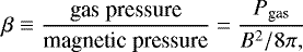
where the field strength B is given in Gauss and the pressure in dyn cm−2, we find a value of β ≈ 0.002 at the bottom of the atmosphere (logτ5000 = +2.0) of HD 119419, decreasing outwards (logτ5000 = −4.0) to some 10−7. In the case of HD 32633, we find β ≈ 0.004 in the deepest layers, β ≈ 3 × 10⁻⁷ farther up. Even a star like 49 Cam, with field strengths of only 6.5 kG maximum (Silvester et al. 2017) features β ≈ 0.015 deep down and 9 × 10⁻⁵ in high layers. These values should not be taken too literally (it seems unlikely that the magnetic field remains constant over the whole vertical extension of the atmosphere) but they certainly give valid indications as to the importance of the magnetic field and the necessity to treat it as force free.
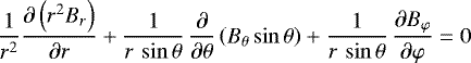
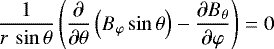
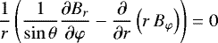
In the past, when modelling of the magnetic geometries of CP stars was restricted to dipolar and dipolar plus quadrupolar configurations, the force-free condition was always automatically satisfied, also in the case of Stift’s tilted, excentric dipole model (Stift 1975; Stift et al. 2013). It is true that force-free stellar magnetospheres have already been considered decades ago (Goossens & Hereygers 1985), and were applied to the modelling of four well-known CP stars by Stift & Goossens (1991). Since the introduction of ZDM, however, the force-free condition has never been mentioned or taken into account, Braithwaite & Spruit (2017) being to our knowledge the only exception. Spruit (priv. comm.) emphasises the important fact that the construction of a force-free field is not possible in terms of a boundary-value problem; force-free fields must be understood in the context of the entire history of the fluid displacements at their boundary. It follows that within the framework of ZDM, it is not possible to determine the shape of a general force-free configuration; the inversion of strong magnetic fields in CP stars must of necessity be based on purely potential fields, ensuring J = ∇ ∧ B = 0 in addition to zero divergence div B = 0. In spherical coordinates, this leads to
 (1)
(1)
 (2)
(2)
 (3)
(3)
 (4)
(4)
These equations define the relation between the components of the magnetic field vector. Equations (2)–(4) of Jardine et al. (1999) (hereafter JBDC) fulfil the zero divergence and force-free conditions. Donati et al. (2006) (hereafter DHJ) on the other hand – claiming to use a formalism similar to that of JBDC – in their Eqs. (2)–(8) instead define a field made up of poloidal and toroidalcomponents, expanded in spherical harmonics. There has been a confusion between “poloidal” and “potential” in the 2006 paper: the fields are described as “the sum of a potential and a toroidal component”, but later we are told that the authors “generalize the problem to fields that are non-potential and feature a significant toroidal component”. Moira Jardine (priv. comm.) has confirmed that the latter statement is correct; such a non-potential part obviously violates the force-free condition.
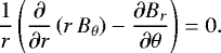
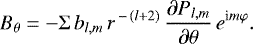
To demonstrate this, we consider the φ-component of the curl for the potential field of JBDC and the poloidal component of the DHJ field, respectively (we discard the toroidal part, which we discuss separately below). Equations (2) and (3) of JBDC read
 (5)
(5)
 (6)
(6)
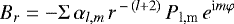
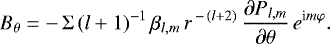
Adding the radial part and omitting a regularisation factor, Eqs. (2)–(3) and (5)–(6) of DHJ give
 (7)
(7)
 (8)
(8)
Whereas the JBDC formulation straightforwardly leads to zero current density, the DHJ field will in general not be force free; only for the very specific case of βl,m = − αl,m do we encounter a potential field and zero current density. Clearly, Eqs. (1)–(3) of Kochukhov et al. (2014) have to be seen in the same light as the DHJ field. In that paper it is stated that the coefficients αl,m, βl,m, and γl,m are free parameters of the harmonic expansion, corresponding to contributions from radial poloidal, horizontal poloidal, and horizontal toroidal magnetic field components, respectively. Even if no toroidal field is assumed in the spherical harmonics expansion, one expects effectively zero likelihood that a ZDM inversion will yield βl,m = − αl,m for all combinations of l and m. As we show in the following section, this expectation is borne out by the published maps of strong-field CP stars.
At this point, it is appropriate to add a very short discussion of the toroidal fields adopted by DHJ. These fields are non-potential and imply electric currents (Winch et al. 2005). How could such fields and currents remain stable for years, possibly for decades? There is very little to be found in the literature concerning large-scale stellar toroidal fields. However, following the arguments of Mestel & Moss (1983), we presume that in the tepid, low-conductivity outer layers of CP stars, observable toroidal fields will decay and disappear over relatively short timescales. Therefore we surmise that the inclusion of a toroidal part in the ZDM procedure for CP stars is not legitimate; adverse effects on the inversion may be expected if done so.
Based on these considerations, it becomes clear that Eqs. (1)–(3) of Kochukhov et al. (2014), although possibly applicable to very weak stellar fields, are not suited for the modelling of stars like HD 32633 (Silvester et al. 2015), 53 Cam (Kochukhov et al. 2004), HD 75049 (Kochukhov et al. 2015), HD 119419 (Rusomarov et al. 2018), HD 125428 (Rusomarov et al. 2016), HD 133880 (Kochukhov et al. 2017), 49 Cam (Silvester et al. 2017), and α2 CVn (Silvester et al. 2014). All the published Zeeman Doppler maps of these CP stars with strong fields have thus been obtained with an incorrect set of formulae. It follows that these magnetic maps are spurious in their entirety, and so are the corresponding abundance maps, because Zeeman splitting, Zeeman intensification, and polarisation of the spectral lines are based on erroneous magnetic field values. The situation is not quite so clear-cut with stellar fields of more moderate strength, but as Spruit (priv. comm.) points out, these are probably also stable on very long timescales so that Ohmic diffusion has given the field in the atmosphere sufficient time to relax to its lowest energy state, that is, a potential field.
3 Published versus force-free maps
Geophysicists modelling the earth’s magnetism do not restrict the dissemination of their results to plots in journals and on web-pages, rather they provide extensive tables, Fortran codes with hundreds of lines of data, notebooks, and so on. This allows fellow scientists to take advantage of the existing wealth of models for further investigations; it also constitutes a useful check on the integrity of data and models. In ZDM, not even the coefficients of the spherical harmonics expansion of any of the many CP stars analysed have ever been made available, apart from those for 36 Lyn (Oksala et al. 2018). Over the years, there has been no way to obtain ZDM data in view of an independent assessment of the published maps and of further analyses.
Fortunately, things have changed recently thanks to the routine availability of high-quality colour plots in online publicationsand to powerful interpreted computing languages. A few transformations applied to the published ZDM maps sufficeto recover magnetic field geometries to a gratifying degree of reliability. Figure 1 (left top) shows the radial field of HD 32633 as reconstructed from the maps published by Silvester et al. (2015), Fig. 1 (right top) the horizontal field. Below to the left we show a spherical harmonics fit with l = 1−9 applied to the recovered map of the radial magnetic field. For all practical purposes, the data underlying the Hammer projections in these plots are near enough to the results obtained with the INVERS10 code to be used straightforwardly in further analyses. We know that in the case of potential poloidal (and thus force-free) fields, the horizontal field components can be derived directly from the radial field (see e.g. Winch et al. 2005). For the necessary calculations, we have developed a new code, testing it with the International Geomagnetic Reference Field (Alken et al. 2021). We note that the resulting map (Fig. 1, right middle) of the horizontal field – force free, as required in view of the strong magnetic fields involved – is totally at variance with the original map, which represents a non-potential field with magnetic forces that are not in balance. In an independent analysis of the original magnetic maps, C.D. Beggan (British Geological Survey, Edinburgh) has confirmed that from the raw published radial field maps, one cannot reproduce the horizontal or modulus plots shown in the paper (Fig. 1, bottom left and right). However, we clarify that our reasoning is not based on the assumption that the radial field is correct; it is the incompatibility between radial and horizontal field that is decisive.
We also studied HD 119419 (Rusomarov et al. 2018) with its magnetic field modulus reaching about 26 kG and its spectacular four spots of very low values of the horizontal field. Interestingly, here the spherical harmonics fit to the radial field is somewhat unsatisfactory, the residuals being almost three times as large as for HD 32633. Although we feel unable to explain this discrepancy, Fig. 2 (left) shows a field map sufficiently near to the original one about the equator and in the northern hemisphere to make possible the desired further analyses. Proceeding as for HD 32633 with our well-tested code, we show that the published horizontal field certainly is not force free (Fig. 2, right).
Similar analyses have proved straightforward (Stift, unpublished) for HD 125428 (Rusomarov et al. 2016) and for HD 133880 (Kochukhov et al. 2017). In the case of HD 75049 (Kochukhov et al. 2015), on account of the low inclination i = 30°, it will be much more difficult to obtain the direct proof of a violation of the force-free condition despite the extreme field strengths involved.
4 Regularisation functionals for the magnetic field
Both in the mapping of 2D horizontal abundance maps and in the derivation of vector magnetic field maps of CP stars, Tikhonov regularisation currently is the only or main constraint in use. In their Eq. (5), Kochukhov & Wade (2010) minimised simultaneously the double sum of the squared differences between all combinations of two magnetic vectors and all combinations of two abundances of the chemical elements considered in the inversion. We note that there is not a single test to be found in the literature that would demonstrate how this Tikhonov regularisation could possibly ensure the correct recovery of a force-free or even just divergence-free magnetic field. The test cases presented by Kochukhov & Piskunov (2002) exclusively concern a dipole of 8 kG (!) polar strength and a few models with an added axisymmetric quadrupole, of 8 kG strength again. Tests with these huge field strengths have been devised in a way as to ensure an ideal combination of inclination, magnetic geometry, and rotational velocity for the application of MDI; therefore they cannot provide answers for more general magnetic geometries.
In the context of later inversions, where spherical harmonics are fitted to the observed magnetic field, Kochukhov et al. (2014) have had recourse to a new penalty function intended to suppress unnecessary higher-order modes. They chose the expression Σl,m l2 (α2 + β2 + γ2), where α, β, and γ characterise contributions of the radial poloidal, horizontal poloidal, and horizontal toroidal magnetic field components, respectively. Not one test or any theoretical discussion has accompanied the introduction of this functional to show that it would filter out the correct magnetic map among countless rival maps. Shortly afterwards, Rusomarov et al. (2016) presented a penalty function of the form  , again without any accompanying arguments. We are now faced with at least three penalty functions for the magnetic field, all of which constitute largely or even entirely untested constructs, and whose respective performances have never been compared.
All three penalty functions clearly fail to lead to physically feasible field geometries in strongly magnetic CP stars. Although a current-free magnetic field could in principle be obtained by the correct combination of α and β, this obviously is not achieved by any of the regularisation functions in question.
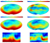 |
Fig. 1 Left: Radial magnetic field of HD32633. From top to bottom: original field recovered from published plots, original field fitted with spherical harmonics, and original field fitted with an independent code by C.D. Beggan (British Geological Survey, Edinburgh). The phases differ by 180° between the two codes. Right: Horizontal magnetic field of HD32633. From top to bottom: original field recovered from published plots, horizontal field derived from the radial field by assuming a potential poloidal force-free configuration, and horizontal field derived similarly with the independent code by C.D. Beggan. |
5 Conclusions
In the past, the magnetic geometries as derived from Stokes IV observations or later from high-resolution and high S/N Stokes IQUV line profiles have escaped close scrutiny. Although the published maps for 53 Cam did not fulfil the condition of zero divergence, there never was a reassessment based on new observations. Later analyses of strongly magnetic BpAp stars took increasing care to ensure zero divergence by fitting spherical harmonics to the magnetic vector field, but as we have shown, the formulae used are incompatible with potential or force-free fields. The huge differences between the published horizontal field maps and the horizontal fields derived from the radial maps – indicative of erroneous formulae used in the inversion – show that there can be no doubt that the published magnetic (and abundance) maps of CP stars with strong magnetic fields are spurious.
In view of the results obtained in the course of this study, the reserved outlook for ZDM presented by Stift & Leone (2017) has not really improved. Reanalysing – this time based on the correct formulae – well-observed stars with strong magnetic fields is a prerequisite for progress in this field. Once the field determined to a first, rough approximation, extensive simulations with theoretical field-dependent, vertical abundances would allow us to obtain an idea of the possible effects of such variable stratifications on ZDM results, both magnetic and chemical. It is not surprising that simple recipes such as those adopted so far have runinto difficulties and have turned out to be of little help in constraining theoretical and numerical results.
Theory needs observational constraints. The next years will probably show whether these can be provided by improved ZDM techniques or whether entirely new techniques are needed to unravel the mystery of the “true” magnetic and abundance maps of CP stars.
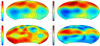 |
Fig. 2 Left, top to bottom: Original radial and horizontal magnetic field of HD119419. Right, tobp to bottom: Corresponding force-free radial and horizontal magnetic field. |
Acknowledgements
Thanks go to the anonymous referee for most constructive criticism and comments. M.J.S. expresses his gratitude toDr. S. Bagnulo for having reawakened his interest in ZDM and initiated a collaboration involving Armagh Observatory whose former director, Prof. M. Bailey, has generously provided unflinching support. We are much obliged to Dr. Patrick Alken (CIRES, Boulder, CO) and to Dr. Ciaran D. Beggan (British Geological Survey, Edinburgh) for clarifying issues concerning magnetic models of the earth and their application to magnetic CP stars. Dr. Dennis Westra https://www.mat.univie.ac.at/~westra/ patiently introduced M.J.S. to some of the intricacies of the associated Legendre functions. We are greatly indebted to Prof. H.C. Spruit for illuminating discussions. Financial contribution from the Programma ricerca di Ateneo UNICT 2020-22 linea 2 is graciously acknowledged. This work would never have been possible without the marvellous public GNAT Ada compiler of AdaCore.
References
- Alfvén, H. 1942, Nature, 150, 405 [Google Scholar]
- Alken, P., Thébault, E., Beggan, C. D., et al. 2021, Earth Planets Space, 73, 49 [NASA ADS] [CrossRef] [Google Scholar]
- Braithwaite, J., & Spruit, H. C. 2017, R. Soc. Open Sci., 4, 160271 [Google Scholar]
- Donati, J. F., Howarth, I. D., Jardine, M. M., et al. 2006, MNRAS, 370, 629 [NASA ADS] [CrossRef] [Google Scholar]
- Goossens, M., & Hereygers, G. 1985, A&A, 149, 253 [NASA ADS] [Google Scholar]
- Jardine, M., Barnes, J. R., Donati, J.-F., & Collier Cameron, A. 1999, MNRAS, 305, L35 [NASA ADS] [CrossRef] [Google Scholar]
- Kochukhov, O., & Piskunov, N. 2002, A&A, 388, 868 [CrossRef] [EDP Sciences] [Google Scholar]
- Kochukhov, O., & Wade, G. A. 2010, ApJ, 513, A13 [Google Scholar]
- Kochukhov, O., Bagnulo, S., Wade, G. A., et al. 2004, A&A, 414, 613 [NASA ADS] [CrossRef] [EDP Sciences] [Google Scholar]
- Kochukhov, O., Lüftinger, T., Neiner, C., Alecian, E., & MiMeS Collaboration 2014, A&A, 565, A83 [NASA ADS] [CrossRef] [EDP Sciences] [Google Scholar]
- Kochukhov, O., Rusomarov, N., Valenti, J. A., et al. 2015, A&A, 574, A79 [NASA ADS] [CrossRef] [EDP Sciences] [Google Scholar]
- Kochukhov, O., Silvester, J., Bailey, J. D., Landstreet, J. D., & Wade, G. A. 2017, A&A, 605, A13 [NASA ADS] [CrossRef] [EDP Sciences] [Google Scholar]
- Mestel, L., & Moss, D. L. 1983, MNRAS, 204, 575 [NASA ADS] [CrossRef] [Google Scholar]
- Oksala, M. E., Silvester, J., Kochukhov, O., et al. 2018, MNRAS, 473, 3367 [NASA ADS] [Google Scholar]
- Piskunov, N. 2001, ASP Conf. Ser., 248, 293 [NASA ADS] [Google Scholar]
- Rusomarov, N., Kochukhov, O., Ryabchikova, T., & Ilyin, I. 2016, A&A, 588, A138 [NASA ADS] [CrossRef] [EDP Sciences] [Google Scholar]
- Rusomarov, N., Kochukhov, O., & Lundin, A. 2018, A&A, 609, A88 [NASA ADS] [CrossRef] [EDP Sciences] [Google Scholar]
- Silvester, J., Kochukhov, O., & Wade, G. A. 2014, MNRAS, 440, 182 [NASA ADS] [CrossRef] [Google Scholar]
- Silvester, J., Kochukhov, O., & Wade, G. A. 2015, MNRAS, 453, 2163 [NASA ADS] [CrossRef] [Google Scholar]
- Silvester, J., Kochukhov, O., Rusomarov, N., & Wade, G. A. 2017, MNRAS, 471, 962 [NASA ADS] [CrossRef] [Google Scholar]
- Stift, M. J. 1975, MNRAS, 172, 133 [NASA ADS] [CrossRef] [Google Scholar]
- Stift, M. J. 1996, IAU Symp., 176, 61 [NASA ADS] [Google Scholar]
- Stift, M. J., & Goossens, M. 1991, A&A, 251, 139 [NASA ADS] [Google Scholar]
- Stift, M. J., & Leone, F. 2003, A&A, 398, 411 [NASA ADS] [CrossRef] [EDP Sciences] [Google Scholar]
- Stift, M. J., & Leone, F. 2017, ApJ, 834, 24 [Google Scholar]
- Stift, M. J., Hubrig, S., Leone, F., & Mathys, G. 2013, ASP Conf. Ser., 479, 125 [NASA ADS] [Google Scholar]
- Tiwari, S. K. 2012, ApJ, 744, 65 [NASA ADS] [CrossRef] [Google Scholar]
- Vogt, S. S., Penrod, G. D., & Hatzes, A. P. 1987, ApJ, 321, 496 [Google Scholar]
- Winch, D. E., Ivers, D. J., Turner, J. P. R., & Stening, R. J. 2005, Geophys. J. Int., 160, 487 [NASA ADS] [CrossRef] [Google Scholar]
All Figures
|
Fig. 1 Left: Radial magnetic field of HD32633. From top to bottom: original field recovered from published plots, original field fitted with spherical harmonics, and original field fitted with an independent code by C.D. Beggan (British Geological Survey, Edinburgh). The phases differ by 180° between the two codes. Right: Horizontal magnetic field of HD32633. From top to bottom: original field recovered from published plots, horizontal field derived from the radial field by assuming a potential poloidal force-free configuration, and horizontal field derived similarly with the independent code by C.D. Beggan. |
| In the text | |
|
Fig. 2 Left, top to bottom: Original radial and horizontal magnetic field of HD119419. Right, tobp to bottom: Corresponding force-free radial and horizontal magnetic field. |
| In the text | |
Current usage metrics show cumulative count of Article Views (full-text article views including HTML views, PDF and ePub downloads, according to the available data) and Abstracts Views on Vision4Press platform.
Data correspond to usage on the plateform after 2015. The current usage metrics is available 48-96 hours after online publication and is updated daily on week days.
Initial download of the metrics may take a while.