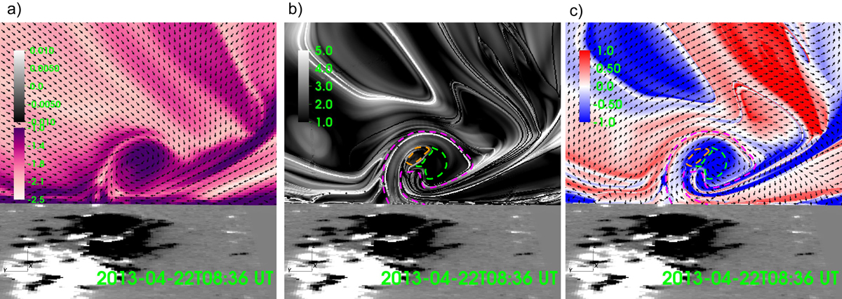
Simulation parameters at slice x = 76 Mm revealing the existence of a flux rope system on 22 April 2013 at 08:36 UT, just before the onset of the eruption discussed in Sect. 2.2. Panel a: logarithm of the current density scaled by the magnetic field magnitude log₁₀(J/B) (white-purple color, saturated at −2.5 and −1) and the direction of the magnetic field projected to the plane B_yz/B_yz| as black arrows. The B_z component is plotted at the lower (z = 0) photospheric boundary of the simulation in black-white coloring saturated at ±0.01 T(=±100 Mx cm⁻²). Panel b: log-scaled magnetic squashing factor log₁₀Q (black-white color, saturated at 1 and 5). Panel c: twist number of the magnetic field lines T_w (blue-red color, saturated at −1 and 1) and the direction of the Lorentz force projected to the plane (J × B)_yz/|(J × B)_yz| as black arrows. The lime and orange dashed curves in panels b and c enclose the regions over which the field lines of the observed flux rope system pass the x = 76 Mm plane. The lime curve encloses the main FR and the orange curve the intertwined FR (see text for exact definitions). Magenta dashed curves in these panels show the QSL boundary enclosing the FR system (also illustrated in Fig. 7b). Animated versions of each panel are available online.